Article

Performance and Feasibility of Drone-Mounted Imaging Spectroscopy for Invasive Aquatic Vegetation Detection

1
Earth Observation and Remote Sensing Lab., University of California, Merced, 5200 Lake Rd., Merced, CA 95341, USA
2
California Department of Fish and Wildlife, 2109 Arch Airport Rd., Stockton, CA 95206, USA
*
Author to whom correspondence should be addressed.
Remote Sens. 2021, 13(4), 582; https://doi.org/10.3390/rs13040582
Submission received: 17 December 2020 / Revised: 25 January 2021 / Accepted: 4 February 2021 / Published: 6 February 2021

Abstract

:
Invasive plants are non-native species that can spread rapidly, leading to detrimental economic, ecological, or environmental impact. In aquatic systems such as the Sacramento-San Joaquin River Delta in California, USA, management agencies use manned aerial vehicles (MAV) imaging spectroscopy missions to map and track annual changes in invasive aquatic plants. Advances in unmanned aerial vehicles (UAV) and sensor miniaturization are enabling higher spatial resolution species mapping, which is promising for early detection of invasions before they spread over larger areas. This study compared maps made from UAV-based imaging spectroscopy with the manned airborne imaging spectroscopy-derived maps that are currently produced for monitoring invasive aquatic plants in the Sacramento-San Joaquin Delta. Concurrent imagery was collected using the MAV mounted HyMap sensor and the UAV mounted Nano-Hyperspec at a wetland study site and classification maps generated using random forest models were compared. Classification accuracies were comparable between the Nano- and HyMap-derived maps, with the Nano-derived map having a slightly higher overall accuracy. Additionally, the higher resolution of the Nano imagery allowed detection of patches of water hyacinth present in the study site that the HyMap could not. However, it would not be feasible to operate the Nano as a replacement to HyMap at scale despite its improved detection capabilities due to the high costs associated with overcoming area coverage limitations. Overall, UAV-based imaging spectroscopy provides comparable or improved capability, and we suggest it could be used to supplement existing monitoring programs by focusing on target areas of high ecologic or economic priority.

1. Introduction

Invasive plants are a rapidly growing global concern due to their negative ecological and economic impacts. The introduction of invasive plants often results in the extinction of native plants and a reduction in biodiversity, either by outcompeting or hybridizing with native species [1,2,3]. Under most scenarios, invasive plants arrive without their co-evolved competitors or parasites allowing them to spread rapidly, replacing native plants without assuming their ecological roles. Plant invasions have been shown to modify ecosystem processes such as nutrient availability, nutrient cycling, soil chemistry, water tables, hydrology, food waste, and habitats [4]. Management of these potentially detrimental impacts is complicated by changes in climate [5] and intensified by increases in invasion frequency due to globalization [6,7]. Human-mediated introductions of invasive plants are most common and tend to be more rapid, increasing propagule pressure and exacerbating the threat of the economic and environmental damages associated with invasive plants [8,9,10].
Over a decade and a half ago, global costs associated with the management of invasive plants were estimated at $34.6 billion as a result of approximately 25,000 foreign plants, and costs are bound to be higher now as globalization has increased [2]. To mitigate the economic and environmental damage, governmental cooperation and management on national and international levels are required. The United Nations Sustainable Development Goal 15, Life on Land, includes a focus on invasion prevention, control, and eradication [11]. Other governmental bodies such as the European Environmental Agency (EEA) and the United States National Invasive Species Council (NISC) are also working to improve global management capabilities. The EEA has developed indicators summarizing invasion trends and biodiversity threats and the NISC has been attempting to standardize data formats and protocol [1]. Understanding invasion origins, pathways, and processes is a key step in management and require geographic observations.
Imaging spectroscopy, or hyperspectral remote sensing, has become a favored tool for invasive plant species mapping due to its synoptic viewpoint and its proven success in providing sufficient spectral data to differentiate between species within complex communities such as wetlands [12,13,14,15,16,17]. The capability to detect plant traits and species using this technology coupled with map creation is invaluable for monitoring and managing invasive plants [18]. For this reason, airborne imaging spectroscopy campaigns have become a common practice because they offer the spectral information necessary to discriminate between species sharing similar attributes [1] while having moderate to high spatial resolution needed to detect species patches.
Improvements in the technology of unmanned aerial vehicles (UAV) and sensors now offer the potential to fill critical gaps between field surveys and manned flights. Manned flights provide a much larger geographic coverage, but the tradeoff is the loss of the extremely high spatial detail associated with field surveys. UAV sits between this range of capability, providing imagery with a geographic footprint smaller than manned flights but larger than the single points provided by field survey, and are capable of imaging difficult-to-access areas such as wetlands. UAV also have high operational flexibility and low costs relative to manned flights as well as the extensive field campaigns required for field surveys [19,20]. This gives UAV the potential to support more frequent, small-footprint acquisitions. The capability to launch on-demand enables better characterization of phenological stages, differences in phenology between species, and allows sampling during specific events such as floods or herbicide treatments. Multispectral cameras or simply high-resolution RGB (red green blue) cameras are the most commonly used sensors on UAV; however, newer pushbroom imaging spectrometers, such as the Headwall Nano-Hyperspec, (Headwall Photonics, Bolton, MA, USA) with its light weight and high quantity of spectral bands, offers tremendous potential for mapping species. Despite the historical difficulty in achieving consistent spectral and radiometric quality from UAV-mountable line scanners [21], studies have shown success in providing detailed community mapping in notoriously difficult regions such as wetlands [22] and grasslands [23]. However, the question remains of how UAV imaging spectroscopy-generated maps compare with MAV imaging spectroscopy maps, which are routinely used for the management of invasive species.
The objective of this study is to highlight the scientific, operational, and economic feasibility of UAV imaging spectroscopy for invasive species monitoring in wetland environments by comparing the mapping performance of an imaging spectrometer mounted on an UAV to one mounted on a manned aerial vehicle (MAV) that is used routinely for monitoring. The UAV-mounted sensors offer much higher spatial resolution than aircraft-mounted imaging spectrometers but have lower spectral quality, and smaller spectral range, and a smaller spatial footprint due to lens specifications and UAV flight restrictions. Manned airborne campaigns typically have high spectral resolution and range, moderate spatial coverage, and low revisit time due to the complexity of flight planning and costs. The Nano-Hyperspec imaging spectrometer was flown concurrently with the HyMap imaging spectrometer during its annual mission to collect imagery for invasive aquatic plant mapping. The data collected by UAV were used to build a random forest (RF) model and create a thematic map. This was compared with a map created from the MAV data as part of the University of California Davis’s aquatic weed-mapping program in the Sacramento-San Joaquin Delta in California, which follows a similar mapping approach using random forest.

2. Materials and Methods

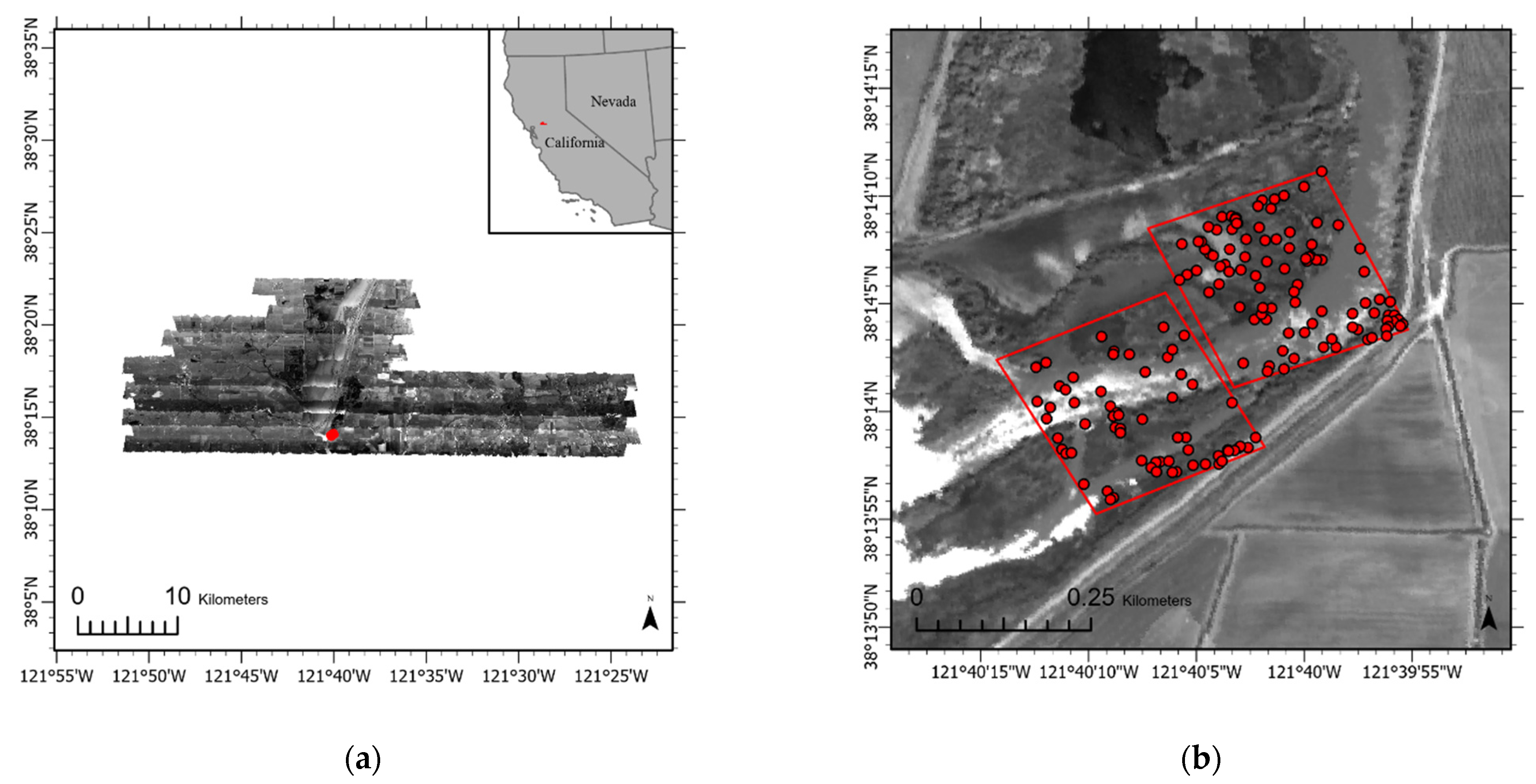
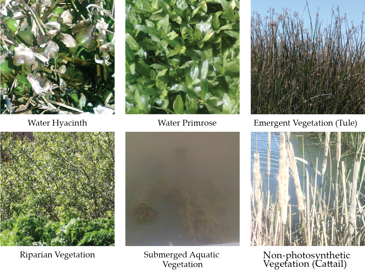
2.1. Study Site and Target Classes

The Sacramento-San Joaquin River Delta, the upstream component of the San Francisco Estuary is the largest tidal freshwater estuary in the western United States. It is a heavily engineered system consisting of complex waterways, reclaimed islands supporting agriculture, and flooded islands that support lake-like and wetland environments. It provides habitat for numerous species and has a disproportionately important role in providing vital ecosystem services [24,25]. It also serves as the major water hub for water in the state. The Delta is also one of the most invaded ecosystems in the world [26]. Invasive aquatic plants have been detrimental to water pumping [27], water quality [28,29], commerce, recreation [30], and have impacted native species [4].
Efforts to map and monitor invasive aquatic plants in the Delta using airborne imaging spectroscopy have been under development dating back to 2003, led by the Center for Spatial Technologies and Remote Sensing (CSTARS) at UC Davis [12,15,16,31]. Imaging spectroscopy data have been collected annually from 2003—2008 and from 2014—to the present and aquatic invasive species mapping is considered near-operational.
A MAV-mounted imaging spectrometer was tasked by CSTARS to collect imagery in April 2019 across the entire Delta. We used this opportunity to collect concurrent UAV-based imaging spectroscopy to compare its mapping capabilities using the near-operational MAV-derived maps as a benchmark. The UAV study area consisted of two roughly 200 × 200 m areas near Miner Slough and the Sacramento Deepwater Shipping Channel, as shown in Figure 1. This region was selected because it contained two invasive aquatic macrophytes as well as other common species or classes found throughout the Delta [32].
Two major floating invasive species of concern in the Delta are water hyacinth (Eichohornia crassipes) and water primrose (Ludwigia spp.). Water hyacinth is a perennial, mat-forming floating aquatic plant that has been a problematic species in the Delta for decades [33]. Mats of water hyacinth can double biomass within 10 days [34], quickly overtaking areas, decreasing water quality and quantity by decreasing dissolved oxygen content and increasing transpiration [31,35], and obstructing waterways for commerce and recreation [36]. Water primrose is a problematic amphibious plant that can form floating mats. Its amphibious capability in addition to fast growth rates has made it a threat to the Delta, endangering native species and wetland restoration projects in the region, as well as posing a threat to humans because primrose mats provide habitats for mosquitos transmitting the West Nile virus [4]. As the primary focus of this investigation, they are the only species-level classes included. Other land cover classes listed in Table 1 were chosen to align with existing classes in HyMap-derived maps created by CSTARS in 2018 [32]. Field photos of the vegetation classes can be seen in Figure 2. The non-photosynthetic vegetation class was added to the Nano map post-classification using a normalized difference vegetation index (NDVI) threshold because it was not identified as a separate class during the ground reference survey.

2.2. Imaging Spectroscopy Data

The Headwall Nano-Hyperspec is a small, 0.5 kg, pushbroom imaging spectrometer that can be mounted on a UAV. It can be purchased as a turnkey package including a DJI M600Pro UAV, DJI Ronin gimbal, calibration tarps, and software (Headwall Photonics, Bolton, MA, USA). The DJI M600Pro is a six-rotor UAV system weighing 10kg with a 1.133 m diagonal wheelbase. It has a maximum take-off weight of 15 kg and an approximately 16-min flight time at that weight. The Nano records radiance in 270 bands of visible and near-infrared light across 400 to 1000 nm. Additional sensor specifications can be found in Table 2. By flying at an altitude of 115 m, the Nano-captured imagery with a 5.1 to 5.4 cm spatial resolution, varying slightly due to ground topography and wind conditions. The imagery was collected between 12:30 and 13:15 PDT on 9 April, 2019. Solar radiation was approximately 907 w/sq.m and windspeed was roughly 11.4 kph during the flights. The UAV was flown over two regions and sixteen flight lines were collected, eight flying into and eight flying away from the solar plane. The raw image cubes collected by the Nano were converted to radiance using a dark calibration of the sensor conducted preflight, then the imagery was orthorectified and converted to reflectance cubes using Headwall’s SpectralView software (Headwall Photonics, Bolton, MA, USA) along with a reflectance tarp, and ENVI 5.5 (L3 Harris Geospatial, Boulder, CO, USA).
The HyMap sensor, operated by HyVista is a whiskbroom sensor system consisting of an Si detector array and three InSb array modules that provide contiguous spectral sampling across the visible, near-infrared, and shortwave infrared regions. It has a 60° field of view (FOV) with an instantaneous field of view (IFOV) of 2.5 mr along-track and 2.0 mr across-track mounted on a gyro-stabilized platform and the detector array has 512 pixels [38]. From 9th to 12th of April 2019, HyVista flew HyMap over the Sacramento-San Joaquin Delta. The data were collected with a ground resolution of 1.7 m with a 20% overlap in flight lines. HyVista performed geo-correction and atmospheric correction using proprietary HyCorr software, an ATREM-based model for correction to apparent surface reflectance and delivered the data to CSTARS at UC Davis for further processing. CSTARS currently uses a random forest machine learning algorithm for their near-operational aquatic weed mapping. CSTARS provided the classified HyMap raster for use in this study.

2.3. Ground Reference Data

Plant species geolocations of the target classes in Table 1 were collected during the week following the concurrent flight on 16–18 April for use in training for Nano thematic classification. Using a 2017 HyMap classification map obtained from CSTARS, a stratified random sampling scheme was used to create 200 points –10 points per class per flight box to visit in the field and record [39]. This sampling design was chosen to maintain random sampling as best as possible while still collecting a sufficient number of samples from each class. Of the 200 ground reference points created, 84 were accessible via a Zodiac Mk. II inflatable boat. At these points the target classes present were documented, photos were taken, and additional information regarding patch sizes and the surrounding area was recorded. A Trimble Geo7X RTK kit with a Zephyr-3 antenna was used to record global navigation satellite system (GNSS) location. Because of the high spatial resolution of the Nano-Hyperspec imagery, great effort was taken to maximize positional accuracy of this survey, and corrected GNSS coordinates fell within a 10 cm range after conducting a differential correction using GPS Pathfinder Office (Trimble, Sunnyvale, CA, USA). Class imbalance or low quantities of reference data for classes has been shown to hinder the performance of classifiers [40], thus points not accessible via watercraft were labeled using a photographic and spectral interpretation of the UAV collected imagery aided by Google Earth Imagery and USDA National Agriculture Imagery Program (NAIP) aerial imagery. There were very few water hyacinth ground reference points and many patches were senescent during the April survey. To compensate for this, additional datapoints were added for the water hyacinth class by creating vegetation patch polygons in the UAV imagery. Then points were randomly sampled from those polygons to provide additional 12 reference points, totaling 179 ground reference points within the study region, as shown in Figure 1B.

2.4. Classifier

RF models [41] are a popular choice for remote sensing for the classification of species from various types of imagery [1] because they have been successfully used to produce high accuracy classifications in complex environments [42,43,44]. Support vector machine algorithms (SVM) [45] are another popular classification method that has been used successfully for mapping species as well [46,47] and there is evidence suggesting that improved performance of RF or SVM over the other may be dependent on the target classes [48]. RF was selected as the classification method by CSTARS for monitoring invasive species in the Delta after nearly a decade of research and development. Previous approaches include statistical modeling, multiple endmember spectral mixture analysis, supervised classification techniques such as spectral angle mapping, boosted regression trees, and biophysical models [4,12,16,49,50,51]. Based on this previous success, RF was also chosen as the classification method for this study. The RF models used to classify the Nano data were constructed and evaluated using the caret [52] and randomForest [53] packages in the R programming language (R Foundation for Statistical Computing, Vienna, Australia).
Although RF often have improved classification accuracies over other methods, they lack a direct quantification error [54]. However, it is important to quantify RF uncertainty because poor model inputs can cause considerable errors in classification [55] and random forests are sensitive to spatial autocorrelation [56]. To account for this, a bootstrapping procedure of building multiple random forests for each model was used to capture the range of accuracies of the RF, where the model run randomly selected a different sample of training and independent test data. After bootstrapping the RF models, accuracies metrics for each model were examined, including overall accuracy, producer’s accuracy, and user’s accuracy [57], as well as Cohen’s Kappa statistic [57]. Overall, accuracy is a measure of the total number of correct class predictions relative to the total quantity of predictions. Producer’s accuracy is a measure of how well a predicted class matches labeled reference data, comparable to a true positive rate. User’s accuracy is a measure of how often predictions are misclassified similar to the positive predictive value. Kappa is an adjusted overall accuracy metric that incorporates a random chance that classification will match its labeled reference data. Kappa was calculated for comparison purposes but otherwise is not discussed in this study due to its similar functionality to overall accuracy [58,59].

RF Modeling

The RF model inputs included reflectance data, occurrence texture data, a forward minimum noise fraction (MNF) transformation, 80 spectral indices (Table S1), and object-based image segments. Occurrence textures metrics and forward MNF transformation were calculated using ENVI 5.5. The 80 spectral indices included are associated with plant biophysical properties. They were calculated using the R programming language, and the formulae from the hsdar package [60]. Object-based image segments were calculated using a Large-Scale Mean-Shift of the green, red, NIR bands in the segOptim package [61] in R utilizing the Orfeo ToolBox [62]. Segmentation parameters were optimized using an iterative procedure [63,64]. After rigorous testing, 1000 trees were selected to use in the RF algorithm
Two small experiments were performed to determine the impact of training and test data quantities and imagery acquisition direction on RF accuracy and uncertainty. Different proportions of labeled data for training and testing were examined in a bootstrapped approach to evaluate the effects of training data quantity and quality on model performance. Test data quantities were varied from 15–55% and training data quantities from 85–45% and for each split, 1000 RF models were built based upon the random selection of training and independent test data. To determine if flight direction had an effect on model performance, training and test data were restricted based on flight direction: toward the solar plane, away from the solar plane, or both. The best performing experimental parameters were then used in the final model set. A flow diagram of the entire classification process is shown in Figure 3.
In addition to reducing the computational burden of so many variables, there is evidence that reducing data dimensionality does not decrease RF performance [65]. Therefore, variable importance based upon the mean decrease in accuracy and the mean decrease in GINI was used to winnow the number of input variables from 1700 to the 500 used in the final classification model.

2.5. Mapping

The ‘best’ performing model was selected from the bootstrapped sets and used to classify the imagery. To improve spatial coherency of the Nano thematic map, post-classification clumping using a 3 × 3 pixel window to eliminate isolated pixels in ENVI 5.5. NPV (non-photosynthetic vegetation) was excluded from the classification originally because the goal was to identify the class present in as much detail as possible regardless of health. To compare the classification maps, all vegetation classes with an NDVI threshold of below 0.3 were reclassified as NPV.

Map Comparisons

The Nano and HyMap thematic maps were compared in three ways:
  • Class Area
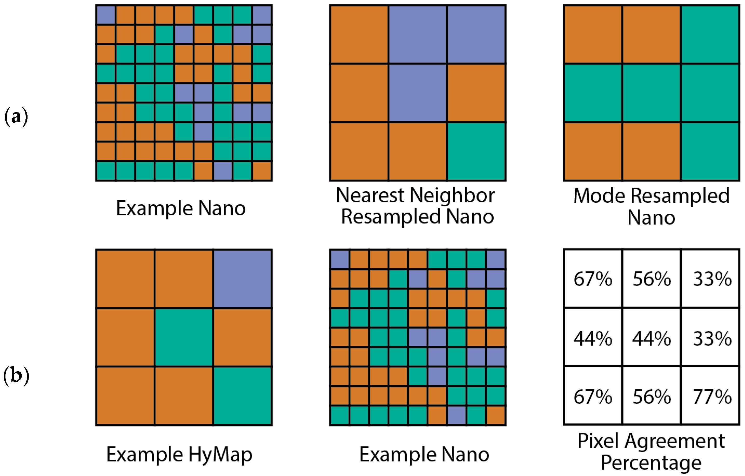
  • Percentage of Nano pixels in agreement with HyMap pixels
  • Upscaled Nano agreement with HyMap
The class area comparison neglects a positional component but highlights variation which may be due to differences in minimum mapping unit, especially for rare classes. The second method, percent pixel agreement, quantified the frequency of different classes from the Nano map occurring within each HyMap pixel, and then compared the percentage of Nano pixels that agree with each HyMap pixel as seen in Figure 4. The third comparison upscaled the Nano map to the HyMap resolution in two ways: The nearest neighbor resampling, and a mode resampling, which reclassified pixels in the Nano map based upon the mode of the Nano pixels occurring within a HyMap pixel as shown in Figure 4. Both were compared using a confusion matrix using the HyMap map as a reference.

3. Results

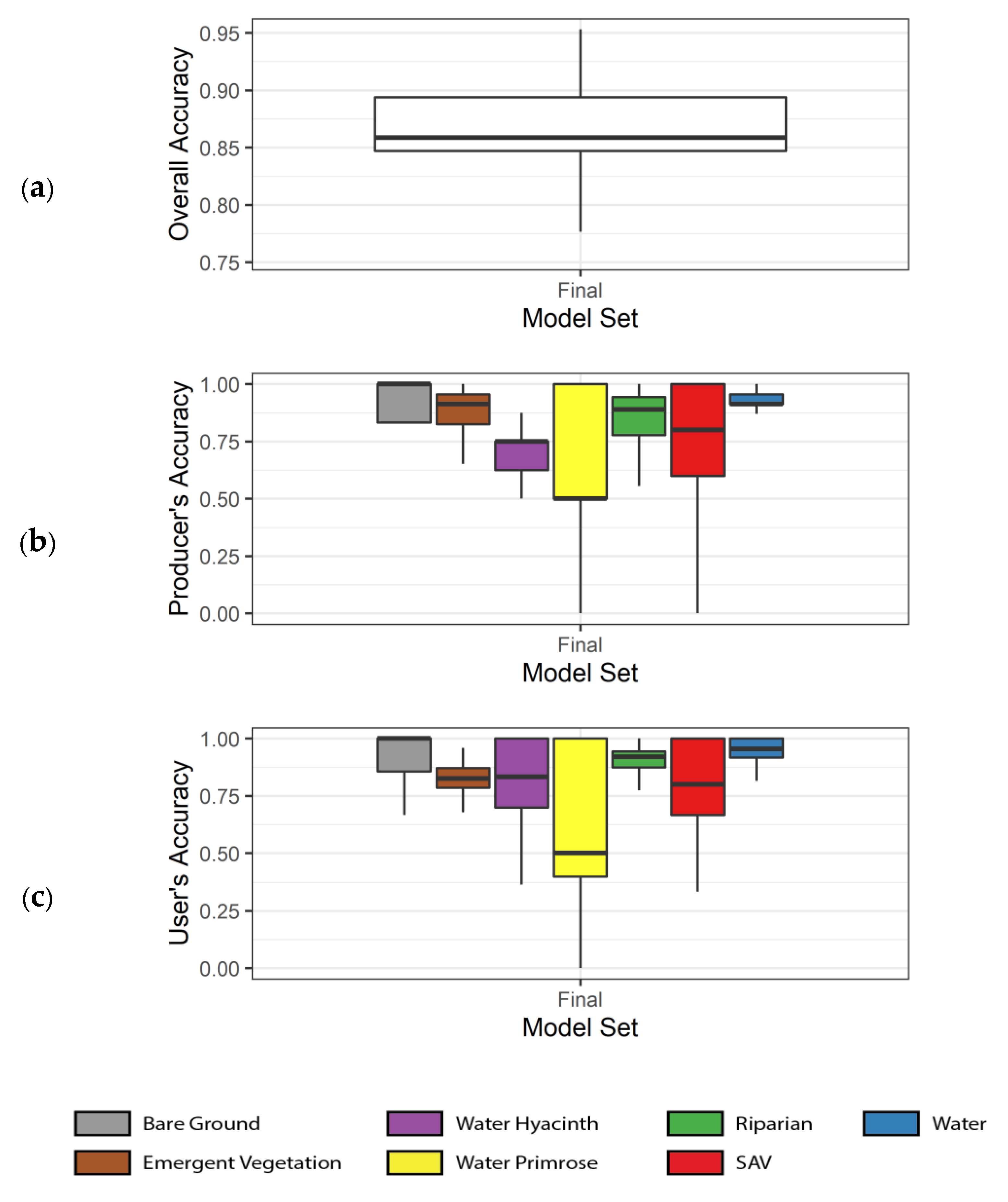
3.1. Model Accuracies

The map-making model selected for classification of the Nano imagery had an overall accuracy of 94.1%, performing better than the HyMap classification for 2019, which had an overall accuracy of 85.7%. Overall accuracies and Kappa values for the Nano and HyMap classification models can be seen in Table 3. For water hyacinth, the Nano classification had a producer’s accuracy of 87.5%, and user’s accuracy of 100%, while in 2019 the HyMap classification had a producer’s accuracy of 93.2% and a user’s accuracy of 89.9%. For water primrose, the Nano classification had a producer’s accuracy of 100% and a user’s accuracy of 50%, while the HyMap classification separated water primrose into two classes based upon density, producer’s accuracies of 90.4% and 74.6%(high and low density, respectively) and user’s accuracies of 94.9% and 94.4% (high and low density, respectively).
The selected classification model for the Nano data was from the upper quantile of accuracies in the final bootstrapped model set. The final set was built using a training/test split of 65/35% and was trained with flights in the toward solar plane direction applied to imagery collected during fight away from the solar plane. The set had a median overall accuracy of 82% as shown in Figure 5. Overall accuracy ranged from 75.3% to 95.3% encompassing the overall accuracies of the HyMap classification in Table 3. Median species-specific producer’s accuracies were all over 75% with the exception of water primrose. Median user’s accuracies showed a similar trend, with water primrose accuracy again being the lowest.

3.2. Variable Reduction and Importance
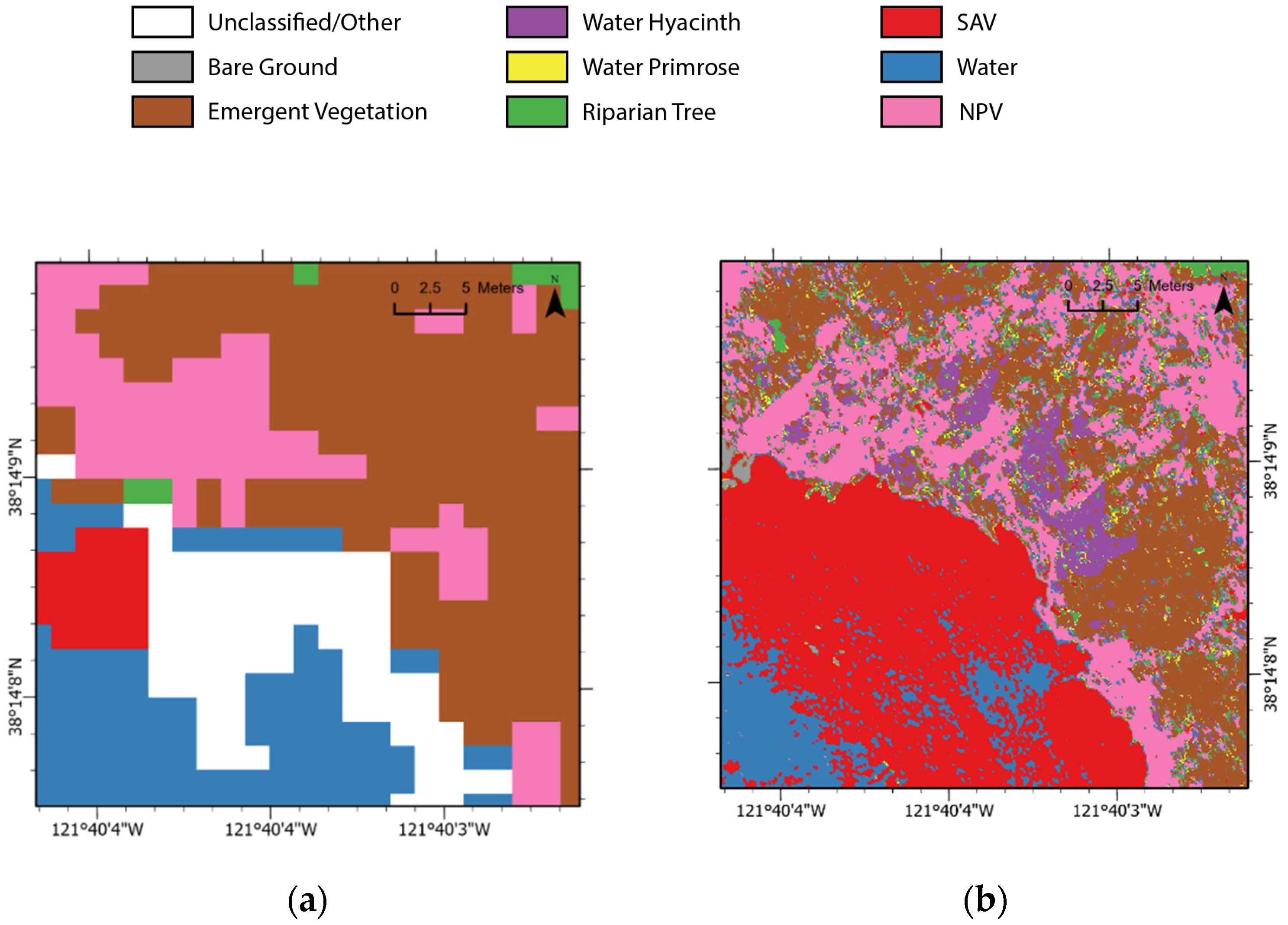
Reducing the overall quantity of variables from 1702 to 500 had no effect on the median overall accuracy of the bootstrapped model sets. There was, however, a significant change in the distribution of accuracies based upon a Chi-squared (χ2) test for independence (χ2 = 23.609, df = 1, p < 0.01) [66]. The bootstrapped model sets with 500 variables had a broader distribution of values. Species-specific accuracies trended accordingly, maintaining a similar median accuracy after variable reduction but increasing in variance.
Spectral indices proved to be the most common variables with high importance and a list of those used can be found in Figure 6. Several are narrow-band vegetation indices related to chlorophyll concentrations and the red edge (Table S1), highlighting the importance of hyperspectral data. The fifth component of the MNF transformation (MNF_5) was the most important variable according to the model, and other important variables were reflectance at 503 nm (RF_503), and mean texture occurrence metrics for bands 50, 52, and 158 (Mean_50, Mean_52, and Mean_158).

3.3. Maps

While a qualitative evaluation of the Nano map compared with the HyMap map shows general agreement, the HyMap classification found no water hyacinth, one of the focal invasive plant targets known to be present in the study area, while the Nano did detect it. The higher spatial resolution of the Nano map is evident, and there is greater detail in the spatial complexity of patches in Figure 7. For example, channels of water flow scouring through the SAV (submerged aquatic vegetation) mats are evident, as are smaller patches on the map. There is also an additional “speckle” in the Nano map. Some of this may be resulting noise/class confusion between classes that have high spectral similarity, such as the emergent class, which contained large amounts of senescent or just greening reed and brushes. But the speckle may also be representative of the highly heterogeneous nature of the environment.

3.3.1. Class Area Comparison

The Nano classification quantified much larger areas of the rare target classes water hyacinth and primrose compared to the HyMap classification. Total class area comparison showed 1589 m2 of water hyacinth within the study site while the HyMap map showed no occurrences as shown in Table 4. The Nano classification found over 300% more water primrose (1617 m2) than the HyMap classification. Additional comparison of class area coverage showed that the classes with the best matchup between the Nano and the HyMap are water, with a roughly 9% difference, and bare ground, with a roughly 8% difference. Riparian shows the third-best agreement with a 15% difference in area coverage, and NPV and SAV show a difference in total area coverage of 25% and 29% respectively. All other classes differed by 30% or more in total area coverage.
Upscaling the Nano maps reduced quantities of the rare target classes of water hyacinth and water primrose. The area of water hyacinth in the resampled Nano map decreased by ten-fold, from 1589 m2 to below 150 m2 with both upscaling methods. Decreases were also substantial for water primrose, from 1617 m2 to 318 m2 for the nearest neighbor resampled area and only 17 m2 for the moving window resampled area.

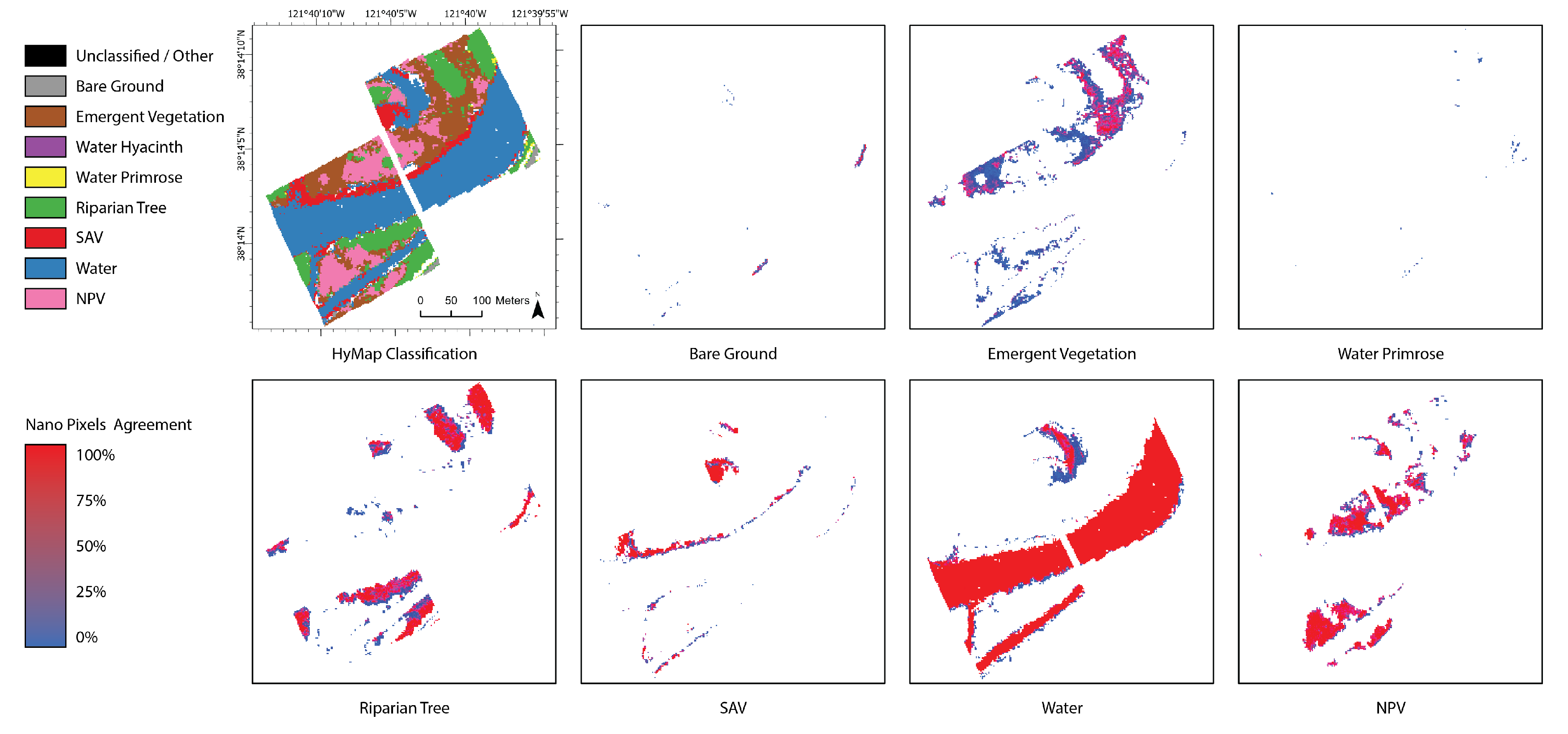
3.3.2. Percent Pixel Agreement

The percent pixel agreement comparison showed a very high level of agreement between more homogenous classes, such as water. Sparsely distributed classes like water primrose had a lower agreement between them. Around the edges of clumps of a class, there was a gradient decline in agreement shown in Figure 8.
When pixel percent agreement was averaged by class, water had the highest agreement between the maps at 88.5%, and water primrose, one of the target classes had almost none, with only 4.17% Additional mean agreement values are in Table 5.

3.3.3. Upscaled Nano Maps Compared to HyMap Comparisons

There was a 71–72% matchup (overall accuracy) between predicted upscaled Nano maps and the predicted HyMap map. Both methods of upscaling the Nano map have a general agreement with the HyMap map, with similar errors of omission and commission across all classes, as seen in Table 6. Errors of omission are the ratio of pixels from each class on the upscaled map that did not match the HyMap map to pixels of that class in the HyMap map, and errors of commission are the ratio of pixels of a class that did not match the HyMap map to the pixels of that class in the upscaled map. Both methods of upscaling eliminated any matchup of the rare, sparsely distributed water primrose class between the maps.

4. Discussion

4.1. Model Accuracies and Comparison

The lower user’s accuracy for water primrose throughout the model set is likely the result of low labeled data quantities and general class sparsity in the study area. From a management standpoint, it is concerning that the user’s accuracy of water primrose from even one of the best performing models was so low; it implies that half of the sites identified would not contain primrose. The consequence could be an increase in operational time for treatment. However, the high producer’s accuracy means that if water primrose were present in the area of concern it would be labeled properly and would not go untreated, a critical piece of information for early intervention and spread control.
The high accuracies for detection of water hyacinth are encouraging, especially because much of the small quantity of water hyacinth present in the study area was senescent at the time of acquisition, which often makes it difficult to differentiate from other senescent vegetation [51]. Mostly senescent water hyacinth also proved problematic for detection by the HyMap model produced by CSTARS, in which reference data from 2018 was used in the 2019 classification because there were too few labeled reference data for water hyacinth in 2019 [42]. This decreased MAV classification performance from the prior year, as seen in Table 3.
There was some confusion between primrose and riparian shrubs due to their similarity in appearance. Within the study site, water primrose appeared mostly inland in the study area and was not flowering at the time the imagery was acquired. However, given its amphibious nature and recent reports of rapid encroachment into upland marsh [4], it may also be the case that this was accurately mapped as a nascent invasion at this site, and the error is associated with an error in the field data in these difficult to access sites.
It is important to note that the selected model accuracies are in the upper quantile of the bootstrapped models, meaning it is unlikely that a repeat study would have a similar result without bootstrapping random forest iterations; but the goal in selection was to create the best map possible to fit the acquired data and the best candidate was selected. This also illustrates the importance of quantifying uncertainty in this, and other machine learning approaches. Low quantities of labeled data also were another probable cause impacting performance for the Nano generated map; however, this is difficult to disentangle from the impacts of not having information in the SWIR. The SWIR has been shown to be a useful predictor for classifying vegetation, specifically for discriminating between SAV, and floating or emergent vegetation [16,67]. This is due to the high absorption of water within this range of the spectrum, and absorption by compounds like cellulose and lignin that help differentiate different structural elements of the canopy [68], especially for floating aquatic plants [15].
The results of the reduction in RF variables aligned with our expectations that data reduction may impact accuracies in various ways but should not drastically reduce performance. The reduction in data was considered a necessity due to the high computational overhead associated with keeping all 1702 variables, a challenge common in the literature of RF classification for remote sensing despite the use of high-performance computing resources [69]. Data reduction has long been an objective of imaging spectroscopy studies to reduce computational overhead and data redundancy [70,71,72] and studies have also shown that data reduction can improve model performance if only the most important variables are retained [73]. RF is relatively robust to redundant input variables [65], though maybe not to correlated predictor variables, which may result in inflated accuracy results [74]. Furthermore, when high dimensional datasets like this one are combined with small amounts of training data, issues such as misclassification due to imbalanced class composition of the training data may be exacerbated [75]. While RF is robust to redundant data, and computational burdens are lessened by the rapid advances and access to HPC computing across the remote sensing community, data volumes continue to grow, especially for extremely high spatial resolution, high spectral resolution UAV-applications. Thus, eliminating redundant and unimportant variables seemed helpful. In this study, the high quantity of spectral data associated with imaging spectroscopy appears useful, especially in the NIR, with several bands in the 740–770 nm region being identified as important. Conversely, this could be a result of the variables being correlated which would inflate accuracy metrics. Common UAV mountable multispectral sensors have a single NIR band located above 800nm which would miss much of this key information. It is also important to consider the effect of lower signal-to-noise ratios in the NIR region of the Nano spectra likely had. Noise increased upon proximity to the largest detectable wavelength (1000 nm) as expected from the sensor specifications (Table 2). The reduced spectral quality of the Nano sensor in this region may have reduced its importance in the model.

4.2. Nano vs. HyMap Maps: How Do They Compare?

Qualitative assessment of the maps suggested that the Nano has the capability to detect smaller patches of species as expected, which is important to locating invasive plants for treatment. This is further supported by in-field experience in the study site and visual assessment of species and quantities present in the area. For example, water hyacinth patches mapped in the Nano imagery were small and mixed with emergent and non-photosynthetic vegetation as shown in the field photo in Figure 9. Furthermore, the water hyacinth in this region was not detected by the HyMap classification but was by the Nano as seen in Figure 10. This highlights the ability of the higher resolution UAV technology to obtain more detailed information, which may be helpful for the management of invasive species in the region.
The quantity of water hyacinth present in the Nano map and absent completely in the HyMap map is significant considering its rapid growth rate [34]. Typically, direct area comparisons are not helpful when assessing classification performance because errors of omission and commission can cancel each other out, in which case having good area matchups between classes may have little meaning [76]. However, in this situation, the area comparison highlighted the usefulness of the Nano’s higher spatial resolution via the detection of water hyacinth and the differences in areal coverage of classes give insight into potentially improved detection capabilities.
Spatially aggregating the Nano data by upscaling using the nearest neighbor approach and the moving window mode resulted in an increase in dominant class abundance and a reduction in minor class abundances. This was unsurprising for the moving window upscale as majority based aggregation typically shows these results [77]. Though not a majority-based aggregation, nearest neighbor resampling chooses the closest point which will have a bias toward dominant classes due to their abundance. The substantial reductions in the class area after upscaling for both water hyacinth and water primrose further illustrate the importance of minimum mapping unit considerations for rare classes, whether they be clumped or dispersed.
The percent pixel agreement shows high agreement in more homogenous areas of the study site while showing lower pixel agreement in more heterogeneous areas, which may hint at better fine-scale detection of sparse or distributed classes from the Nano. The very low agreement of water primrose suggests that it is either being misclassified by the Nano due to lack of reference data or because of the amphibious nature of water primrose, it is spreading into the emergent vegetation making it more difficult to detect using the coarser grain HyMap imagery.

4.3. Management Relevance and Operational Considerations

The capability of the higher spatial resolution UAV based sensors to detect rare classes, such as water hyacinth in this study, is valuable for monitoring management interventions such as early herbicide applications; however, the small footprint of UAV operations would make this process difficult to implement broadly. Specific, targeted deployment at problem areas identified from the previous growing season is likely the best implementation of this process. In addition to the increased detail possible with the UAV, flexibility of deployment could be a benefit. The 2019 HyMap flight over the Delta was conducted in early April, slightly too soon to catch the greening of water hyacinth at a large scale. This is evidenced by the lack of training data reported by CSTARS and their use of data from previous years to map water hyacinth during 2019, likely resulting in their lower accuracies for that year. Maps built using the UAV imagery had a similar accuracy range to that of those created with HyMap during more successful years, but also provided a much higher spatial resolution. As mentioned, the primary disadvantage of using UAV would be the cost and logistics of putting large-scale UAV mapping into practice as approximated in Table 7.
The small spatial footprint of the Nano would require thousands of flights to cover the entire Delta region covered by HyMap, even with multiple UAV units. Table 7 shows estimates of time, data volume, and deployment cost to fly the entire Delta with HyMap and the Nano. For this estimate, the high overlap used in this study to acquire imagery from two directions was abandoned, effectively halving the time estimates, data volume, and associated deployment costs. Even with this reduction, using the Nano to cover the entire Delta would likely be cost-prohibitive. Time estimates include four hours of collection time per day corresponding to solar windows, plus launch preparation time, downloading data, and travel amounting to roughly the other 4 working hours per day. Approximate data volume estimates for HyMap consist of all storage required including intermediate products, as does the Nano data volume. Approximate deployment cost includes initial purchase cost for the Headwall Nano-Hyperspec turnkey package, assumes a team of 3 members, pilot, designated observer, and calibration technician to operate a portable field spectrometer working eight hour days at $20 per hour, a rental vehicle for $60/day, data storage priced at $0.02 per GB, and a 60% overhead. We estimate a UAV survey of the entire Delta would take more than a year to complete with one team, negating much of the advantages of using UAV. This also doesn’t account for the optimal phenological window for target species, which is much narrower than a full year. Multiple teams with multiple units may be able to complete a survey of the entire Delta in a shorter time frame but would have additional costs associated with personnel operating on multiple teams and capital expenditures on multiple pieces of equipment. An additional concern for large-scale usage of the UAV for mapping would be data volume. To cover the entire Delta following the protocols outlined here, roughly 2100 TB of storage space at an estimated cost of $42,238 would be necessary to collect and convert the data to orthorectified reflectance products, not including the storage necessary to create remote sensing products or construct a map, infrastructure many operational agencies invested in invasive species management do not have. The small geographic footprint associated with the high spatial resolution capabilities of UAV imaging spectrometers makes them difficult to implement as a detection method over such a large area. For this reason, if UAV-mounted imaging spectrometers were to be utilized in invasive species management applications, targeted flights in limited locations of high concern or value are recommended.

5. Conclusions

This study outlines a procedure for determining an optimal model and mapping invasive plants in a wetland ecosystem using a Headwall Nano-Hyperspec, and shows the higher spatial resolution provided by the Nano can improve detection of small patches of invasive aquatic plants relative to a near-operational government-funded program. The study demonstrated that a similar methodology applied to data acquired from a UAV-mounted Nano-Hyperspec can result in similar accuracies to the maps made from MAV-mounted imaging spectrometer data. The improved fine-scale detection from UAV does come at a cost, the operational footprint. The small footprint makes coverage of large regions with UAV highly impractical if not impossible, restricting UAV applications to specific areas of concern. One additional advantage of UAV imaging spectroscopy would be on-demand acquisitions. Additional acquisition dates could have been used to Supplement the Information in this study and potentially improve classification accuracy by capturing water hyacinth at a later phenological state when less of it was senescent. This on-demand nature could be useful to management agencies, enabling monitoring after herbicidal treatments and supporting eradication efforts.
In the future, this study may be used as a guide for invasive species mapping using UAV-mounted imaging spectrometers. The capability to detect small patches as shown here is highly useful for weed management applications, as well as mapping that requires fine resolution. Improvement of the orthorectification procedure for the Nano through automation would greatly simplify pre-processing, reduce post-processing labor and make use of the Nano for mapping more practical. Though there are still hurdles to overcome, technological advances will make this application more practical in the near future.

Supplementary Materials

The following are available online at https://www.mdpi.com/2072-4292/13/4/582/s1, Table S1: Vegetation Indices Used.

Author Contributions

E.A.B. designed the study, conducted UAV flight data acquisition, field data acquisition, data analysis and wrote the original draft of the manuscript. E.L.H. contributed to study design, data analysis and writing, and provided equipment and resources to conduct the study. S.K. contributed to the study design, provided the HyMap maps and data, and contributed to review and editing of the manuscript. All authors have read and agreed to the published version of the manuscript.

Funding

This research was funded by internal funds provided by the University of California, Merced School of Engineering.

Data Availability Statement

The data presented in this study are available on request from the corresponding author. The data are not publicly available due to their large size.

Acknowledgments

The authors would like to thank Joshua Viers for providing equipment essential for field data collection and valuable feedback on data analysis. We would also like to thank Christiana Ade for coding expertise, and Brandon Stark, Brandon Genco, Daniel Gomez, Anna Rallings, Zach Yinger, Julia Burmistrova, Jacob Nesslage, Brittany Lopez-Barreto, and Jaycee Martinez for helping with fieldwork operations and data collection. Finally, the authors would like to thank the anonymous reviewers who helped improve this manuscript.

Conflicts of Interest

The authors declare no conflict of interest.

References

  1. Bolch, E.A.; Santos, M.J.; Ade, C.; Khanna, S.; Basinger, N.T.; Reader, M.O.; Hestir, E.L. Remote Detection of Invasive Alien Species. In Remote Sensing of Plant Biodiversity; Cavender-Bares, J., Gamon, J., Townsend, P., Eds.; Springer Nature: Cham, Switzerland, 2020; pp. 267–308. ISBN 978-3-030-33156-6. [Google Scholar]
  2. Pimentel, D.; Zuniga, R.; Morrison, D. Update on the environmental and economic costs associated with alien-invasive species in the United States. Ecol. Econ. 2005, 52, 273–288. [Google Scholar] [CrossRef]
  3. Byers, J.E.; Noonburg, E.G. Scale dependent effects of biotic resistance to biological invasion. Ecology 2003, 84, 1428–1433. [Google Scholar] [CrossRef]
  4. Khanna, S.; Santos, M.J.; Boyer, J.D.; Shapiro, K.D.; Bellvert, J.; Ustin, S.L. Water primrose invasion changes successional pathways in an estuarine ecosystem. Ecosphere 2018, 9, e02418. [Google Scholar] [CrossRef]
  5. Allen, J.M.; Bradley, B.A. Out of the weeds? Reduced plant invasion risk with climate change in the continental United States. Biol. Conserv. 2016, 203, 306–312. [Google Scholar] [CrossRef] [Green Version]
  6. Ricciardi, A. Are modern biological invasions an unprecedented form of global change? Conserv. Biol. 2007. [CrossRef] [PubMed]
  7. Seebens, H.; Blackburn, T.M.; Dyer, E.E.; Genovesi, P.; Hulme, P.E.; Jeschke, J.M.; Pagad, S.; Pyšek, P.; Winter, M.; Arianoutsou, M.; et al. No saturation in the accumulation of alien species worldwide. Nat. Commun. 2017, 8, 14435. [Google Scholar] [CrossRef]
  8. Mortensen, D.A.; Rauschert, E.S.J.; Nord, A.N.; Jones, B.P. Forest Roads Facilitate the Spread of Invasive Plants. Invasive Plant Sci. Manag. 2009, 2, 191–199. [Google Scholar] [CrossRef]
  9. Masters, G.; Norgrove, L. Climate change and invasive alien species. UK CABI Work. Pap. 2010, 1. [Google Scholar]
  10. Hulme, P.E. Invasion pathways at a crossroad: Policy and research challenges for managing alien species introductions. J. Appl. Ecol. 2015, 52, 1418–1424. [Google Scholar] [CrossRef]
  11. UN General Assembly. Transforming our world: The 2030 Agenda for Sustainable Development. United Nations A/RES/70/1. New York, NY, USA, 21 October 2015. Available online: https://www.un.org/en/development/desa/population/migration/generalassembly/docs/globalcompact/A_RES_70_1_E.pdf (accessed on 29 January 2021).
  12. Hestir, E.L.; Khanna, S.; Andrew, M.E.; Santos, M.J.; Viers, J.H.; Greenberg, J.A.; Rajapakse, S.S.; Ustin, S.L. Identification of invasive vegetation using hyperspectral remote sensing in the California Delta ecosystem. Remote Sens. Environ. 2008, 112, 4034–4047. [Google Scholar] [CrossRef]
  13. Jollineau, M.Y.; Howarth, P.J. Mapping an inland wetland complex using hyperspectral imagery. Int. J. Remote Sens. 2008, 29, 3609–3631. [Google Scholar] [CrossRef]
  14. Hunter, P.D.; Gilvear, D.J.; Tyler, A.N.; Willby, N.J.; Kelly, A. Mapping macrophytic vegetation in shallow lakes using the Compact Airborne Spectrographic Imager (CASI). Aquat. Conserv. Mar. Freshw. Ecosyst. 2010, 20, 717–727. [Google Scholar] [CrossRef]
  15. Khanna, S.; Santos, M.J.; Ustin, S.L.; Haverkamp, P.J. International Journal of Remote Sensing An integrated approach to a biophysiologically based classification of floating aquatic macrophytes. Int. J. Remote Sens. 2011, 32, 1067–1094. [Google Scholar] [CrossRef]
  16. Hestir, E.L.; Greenberg, J.A.; Ustin, S.L. Classification trees for aquatic vegetation community prediction using imaging spectroscopy. IEEE J. Sel. Top. Appl. Earth Obs. Remote Sens. 2012, 5, 1572–1584. [Google Scholar] [CrossRef]
  17. Zhao, D.; Jiang, H.; Yang, T.; Cai, Y.; Xu, D.; An, S. Remote sensing of aquatic vegetation distribution in Taihu Lake using an improved classification tree with modified thresholds. J. Environ. Manag. 2012, 95, 98–107. [Google Scholar] [CrossRef]
  18. Santos, M.J.; Khanna, S.; Hestir, E.L.; Andrew, M.E.; Rajapakse, S.S.; Greenberg, J.A.; Anderson, L.W.J.; Ustin, S.L. Use of Hyperspectral Remote Sensing to Evaluate Efficacy of Aquatic Plant Management. Invasive Plant Sci. Manag. 2009, 2, 216–229. [Google Scholar] [CrossRef]
  19. Doughty, C.L.; Cavanaugh, K.C. Mapping coastal wetland biomass from high resolution unmanned aerial vehicle (UAV) imagery. Remote Sens. 2019, 11, 540. [Google Scholar] [CrossRef] [Green Version]
  20. Zhong, Y.; Wang, X.; Xu, Y.; Wang, S.; Jia, T.; Hu, X.; Zhao, J.; Wei, L.; Zhang, L. Mini-UAV-Borne Hyperspectral Remote Sensing: From Observation and Processing to Applications. IEEE Geosci. Remote Sens. Mag. 2018, 6, 46–62. [Google Scholar] [CrossRef]
  21. Turner, D.J.; Malenovsky, Z.; Lucieer, A.; Turnbull, J.D.; Robinson, S.A. Optimizing Spectral and Spatial Resolutions of Unmanned Aerial System Imaging Sensors for Monitoring Antarctic Vegetation. IEEE J. Sel. Top. Appl. Earth Obs. Remote Sens. 2019, 12, 3813–3825. [Google Scholar] [CrossRef]
  22. Banerjee, B.P.; Raval, S.; Cullen, P.J. UAV-hyperspectral imaging of spectrally complex environments. Int. J. Remote Sens. 2020, 41, 4136–4159. [Google Scholar] [CrossRef]
  23. Melville, B.; Lucieer, A.; Aryal, J. Classification of Lowland Native Grassland Communities Using Hyperspectral Unmanned Aircraft System (UAS) Imagery in the Tasmanian Midlands. Drones 2019, 3, 5. [Google Scholar] [CrossRef] [Green Version]
  24. Tabacchi, E.; Correll, D.L.; Hauer, R.; Pinay, G.; Planty-Tabacchi, A.M.; Wissmar, R.C. Development, maintenance and role of riparian vegetation in the river landscape. Freshw. Biol. 1998, 40, 497–516. [Google Scholar] [CrossRef]
  25. Barbier, E.B.; Hacker, S.D.; Kennedy, C.; Koch, E.W.; Stier, A.C.; Silliman, B.R. The value of estuarine and coastal ecosystem services. Ecol. Monogr. 2011, 81, 169–193. [Google Scholar] [CrossRef]
  26. Cohen, A.N.; Carlton, J.T. Accelerating invasion rate in a highly invaded estuary. Science 1998, 279, 555–558. [Google Scholar] [CrossRef] [Green Version]
  27. Khanna, S.; Acuña, S.; Contreras, D.; Griffiths, W.K.; Lesmeister, S.; Reyes, R.C.; Schreier, B.; Wu, B.J. Invasive Aquatic Vegetation Impacts on Delta Operations, Monitoring, and Ecosystem and Human Health. Interag. Ecol. Progr. Newsl. 2019, 34, 8–19. [Google Scholar]
  28. Hestir, E.L.; Schoellhamer, D.H.; Greenberg, J.; Morgan-King, T.; Ustin, S.L. The Effect of Submerged Aquatic Vegetation Expansion on a Declining Turbidity Trend in the Sacramento-San Joaquin River Delta. Estuaries Coasts 2016, 39, 1100–1112. [Google Scholar] [CrossRef] [Green Version]
  29. Tobias, V.D.; Conrad, J.L.; Mahardja, B.; Khanna, S. Impacts of water hyacinth treatment on water quality in a tidal estuarine environment. Biol. Invasions 2019, 21, 3479–3490. [Google Scholar] [CrossRef] [Green Version]
  30. Conrad, J.L.; Chapple, D.; Bush, E.; Hard, E.; Caudill, J.; Madsen, J.D.; Pratt, W.; Acuna, S.; Rasmussen, N.; Gilbert, P.; et al. Critical Needs for Control of Invasive Aquatic Vegetation in the Sacramento-San Joaquin Delta (Report). Delta Stewardship Council. 2020. Available online: https://www.deltacouncil.ca.gov/pdf/dpiic/meeting-materials/2020-03-02-item-4-aquatic-weeds-paper.pdf (accessed on 29 January 2021).
  31. Underwood, E.C.; Mulitsch, M.J.; Greenberg, J.A.; Whiting, M.L.; Ustin, S.L.; Kefauver, S.C. Mapping invasive aquatic vegetation in the sacramento-san Joaquin Delta using hyperspectral imagery. Environ. Monit. Assess. 2006, 121, 47–64. [Google Scholar] [CrossRef]
  32. Ustin, S.L.; Khanna, S.; Lay, M.; Shapiro, K.D. Enhancement of Delta Smelt (Hypomesus transpacificus) Habitat through Adaptive Management of Invasive Aquatic Weeds in the Sacramento-San Joaquin Delta & Suisun; Report; California Department of Water Resources: Sacramento, CA, USA, 2019. [Google Scholar]
  33. Cohen, A.N.; Carlton, J.T. Nonindigenous aquatic species in a United States estuary: A case study of the biological invasions of the San Francisco Bay and Delta (Report). US Fish and Wildlife Service. 1995. Available online: http://bioinvasions.org/wp-content/uploads/1995-SFBay-Invasion-Report.pdf (accessed on 29 January 2021).
  34. Venugopal, G. Monitoring the Effects of Biological Control of Water Hyacinths Using Remotely Sensed Data: A Case Study of Bangalore, India. Singap. J. Trop. Geogr. 2002, 19, 91–105. [Google Scholar] [CrossRef]
  35. Jetter, K.M.; Nes, K.; Tahoe, L. The cost to manage invasive aquatic weeds in the California Bay-Delta. ARE Updat. 2018, 21, 9–11. [Google Scholar]
  36. Toft, J.D.; Simenstad, C.A.; Cordell, J.R.; Grimaldo, L.F. The Effects of Introduced Water Hyacinth on Habitat Structure, Invertebrate Assemblages, and Fish Diets. Estuar. Res. Fed. Estuaries 2003, 26, 746–758. [Google Scholar] [CrossRef]
  37. Santos, M.J.; Anderson, L.W.; Ustin, S.L.; Santos, M.J.; Ustin, S.L.; Anderson, L.W. Effects of invasive species on plant communities: An example using submersed aquatic plants at the regional scale. Biol. Invasions 2011, 13, 443–457. [Google Scholar] [CrossRef] [Green Version]
  38. Cocks, T.; Jenssen, R.; Stewart, A.; Wilson, I.; Shields, T. The hymap TM airborne hyperspectral sensor: The system, calibration and performance. In Proceedings of the 1st EARSeL workshop on Imaging Spectroscopy, Zurich, Switzerland, 6–8 October 1998; pp. 37–42. [Google Scholar]
  39. Ustin, S.L.; Khanna, S.; Lay, M.; Shapiro, K.D. Enhancement of Delta Smelt (Hypomesus transpacificus) Habitat through Adaptive Management of Invasive Aquatic Weeds in the Sacramento-San Joaquin Delta; Report; California Department of Fish and Wildlife: Sacramento, CA, USA, 2018. [Google Scholar]
  40. Mellor, A.; Boukir, S.; Haywood, A.; Jones, S. Exploring issues of training data imbalance and mislabelling on random forest performance for large area land cover classification using the ensemble margin. ISPRS J. Photogramm. Remote Sens. 2015, 105, 155–168. [Google Scholar] [CrossRef]
  41. Breiman, L. Random forests. Mach. Learn. 2001, 45, 5–32. [Google Scholar] [CrossRef] [Green Version]
  42. Ustin, S.L.; Khanna, S.; Lay, M.; Shapiro, K.; Ghajarnia, N. Remote Sensing of the Sacramento-San Joaquin Delta to Enhance Mapping for Invasive and Native Aquatic Vegetation Plant Species; Report; California Department of Water Resources: Sacramento, CA, USA, 2020. [Google Scholar]
  43. Burai, P.; Deák, B.; Valkó, O.; Tomor, T. Classification of Herbaceous Vegetation Using Airborne Hyperspectral Imagery. Remote Sens. 2015, 7, 2046–2066. [Google Scholar] [CrossRef] [Green Version]
  44. Marcinkowska-Ochtyra, A.; Jarocińska, A.; Bzdęga, K.; Tokarska-Guzik, B. Classification of Expansive Grassland Species in Different Growth Stages Based on Hyperspectral and LiDAR Data. Remote Sens. 2018, 10, 2019. [Google Scholar] [CrossRef] [Green Version]
  45. Vapnik, V. Pattern recognition using generalized portrait method. Autom. Remote. Control 1963, 24, 774–780. [Google Scholar]
  46. Atkinson, J.T.; Ismail, R.; Robertson, M. Mapping Bugweed (Solanum mauritianum) Infestations in Pinus patula Plantations Using Hyperspectral Imagery and Support Vector Machines. IEEE J. Sel. Top. Appl. Earth Obs. Remote Sens. 2014, 7, 17–28. [Google Scholar] [CrossRef]
  47. Ghosh, A.; Fassnacht, F.E.; Joshi, P.K.; Kochb, B. A framework for mapping tree species combining hyperspectral and LiDAR data: Role of selected classifiers and sensor across three spatial scales. Int. J. Appl. Earth Obs. Geoinf. 2014, 26, 49–63. [Google Scholar] [CrossRef]
  48. Sabat-Tomala, A.; Raczko, E.; Zagajewski, B. Comparison of Support Vector Machine and Random Forest Algorithms for Invasive and Expansive Species Classification Using Airborne Hyperspectral Data. Remote Sens. 2020, 12, 516. [Google Scholar] [CrossRef] [Green Version]
  49. Santos, M.J.; Hestir, E.L.; Khanna, S.; Ustin, S.L. Image spectroscopy and stable isotopes elucidate functional dissimilarity between native and nonnative plant species in the aquatic environment. New Phytol. 2012, 193, 683–695. [Google Scholar] [CrossRef] [PubMed]
  50. Santos, M.J.; Khanna, S.; Hestir, E.L.; Greenberg, J.A.; Ustin, S.L. Measuring landscape-scale spread and persistence of an invaded submerged plant community from airborne Remote sensing. Ecol. Appl. 2016, 26, 1733–1744. [Google Scholar] [CrossRef]
  51. Khanna, S.; Santos, M.J.; Hestir, E.L.; Ustin, S.L. Plant community dynamics relative to the changing distribution of a highly invasive species, Eichhornia crassipes: A remote sensing perspective. Biol. Invasions 2012, 14, 717–733. [Google Scholar] [CrossRef]
  52. Kuhn, M. Building Predictive Models in R Using the caret Package. J. Stat. Softw. Artic. 2008, 28, 1–26. [Google Scholar] [CrossRef] [Green Version]
  53. Liaw, A.; Wiener, M. Classification and Regression by randomForest. R News 2002, 2, 18–22. [Google Scholar]
  54. Coulston, J.W.; Blinn, C.E.; Thomas, V.A.; Wynne, R.H. Approximating prediction uncertainty for random forest regression models. Photogramm. Eng. Remote Sens. 2016, 82, 189–197. [Google Scholar] [CrossRef] [Green Version]
  55. Loosvelt, L.; Peters, J.; Skriver, H.; Lievens, H.; Van Coillie, F.M.B.; De Baets, B.; Verhoest, N.E.C. Random Forests as a tool for estimating uncertainty at pixel-level in SAR image classification. Int. J. Appl. Earth Obs. Geoinf. 2012, 19, 173–184. [Google Scholar] [CrossRef]
  56. Sinha, P.; Gaughan, A.E.; Stevens, F.R.; Nieves, J.J.; Sorichetta, A.; Tatem, A.J. Assessing the spatial sensitivity of a random forest model: Application in gridded population modeling. Comput. Environ. Urban Syst. 2019, 75, 132–145. [Google Scholar] [CrossRef]
  57. Story, M.; Congalton, R.G. Accuracy Assessment: A User’s Perspective. Photogramm. Eng. Remote Sens. 1986, 52, 397–399. [Google Scholar]
  58. Foody, G.M. Explaining the unsuitability of the kappa coefficient in the assessment and comparison of the accuracy of thematic maps obtained by image classification. Remote Sens. Environ. 2020, 239, 111630. [Google Scholar] [CrossRef]
  59. Pontius, R.G.; Millones, M. Death to Kappa: Birth of quantity disagreement and allocation disagreement for accuracy assessment. Int. J. Remote Sens. 2011, 32, 4407–4429. [Google Scholar] [CrossRef]
  60. Lenhert, L.W.; Meyer, H.; Obermeier, W.A.; Silva, B.; Regeling, B.; Thies, B.; Bendix, J. Hyperspectral Data Analysis in R: The hsdar Package. J. Stat. Softw. 2019, 89, 1–23. [Google Scholar] [CrossRef] [Green Version]
  61. Gonçalves, J.; Pôças, I.; Marcos, B.; Mücher, C.A.; Honrado, J.P. SegOptim-A new R package for optimizing object-based image analyses of high-spatial resolution remotely-sensed data. Int. J. Appl. Earth Obs. Geoinf. 2019, 76, 218–230. [Google Scholar] [CrossRef]
  62. Grizonnet, M.; Michel, J.; Poughon, V.; Inglada, J.; Savinaud, M.; Cresson, R. Orfeo ToolBox: Open source processing of remote sensing images. Open Geospat. Data Softw. Stand. 2017, 2, 15. [Google Scholar] [CrossRef] [Green Version]
  63. Radoux, J.; Defourny, P. A quantitative assessment of boundaries in automated forest stand delineation using very high resolution imagery. Remote Sens. Environ. 2007, 110, 468–475. [Google Scholar] [CrossRef]
  64. Whiteside, T.G.; Boggs, G.S.; Maier, S.W. Comparing object-based and pixel-based classifications for mapping savannas. Int. J. Appl. Earth Obs. Geoinf. 2011, 13, 884–893. [Google Scholar] [CrossRef]
  65. Fox, E.W.; Hill, R.A.; Leibowitz, S.G.; Olsen, A.R.; Thornbrugh, D.J.; Weber, M.H. Assessing the accuracy and stability of variable selection methods for random forest modeling in ecology. Environ. Monit. Assess. 2017, 189, 316. [Google Scholar] [CrossRef]
  66. Pearson, K.X. On the criterion that a given system of deviations from the probable in the case of a correlated system of variables is such that it can be reasonably supposed to have arisen from random sampling. Lond. Edinb. Dublin Philos. Mag. J. Sci. 1900, 50, 157–175. [Google Scholar] [CrossRef] [Green Version]
  67. Hestir, E.L.; Brando, V.E.; Bresciani, M.; Giardino, C.; Matta, E.; Villa, P.; Dekker, A.G. Measuring freshwater aquatic ecosystems: The need for a hyperspectral global mapping satellite mission. Remote Sens. Environ. 2015, 167, 181–195. [Google Scholar] [CrossRef] [Green Version]
  68. Ustin, S.L.; Roberts, D.A.; Gamon, J.A.; Asner, G.P.; Green, R.O. Using imaging spectroscopy to study ecosystem processes and properties. Bioscience 2004, 54, 523–534. [Google Scholar] [CrossRef]
  69. Belgiu, M.; Drăgu, L. Random forest in remote sensing: A review of applications and future directions. ISPRS J. Photogramm. Remote Sens. 2016, 114, 24–31. [Google Scholar] [CrossRef]
  70. Ghamisi, P.; Yokoya, N.; Li, J.; Liao, W.; Liu, S.; Plaza, J.; Rasti, B.; Plaza, A. Advances in Hyperspectral Image and Signal Processing: A Comprehensive Overview of the State of the Art. IEEE Geosci. Remote Sens. Mag. 2017, 5, 37–78. [Google Scholar] [CrossRef] [Green Version]
  71. Kaewpijit, S.; Moigne, J.L.; El-Ghazawi, T. Automatic reduction of hyperspectral imagery using wavelet spectral analysis. IEEE Trans. Geosci. Remote Sens. 2003, 41, 863–871. [Google Scholar] [CrossRef]
  72. Agarwal, A.; El-Ghazawi, T.; El-Askary, H.; Le-Moigne, J. Efficient hierarchical-PCA dimension reduction for hyperspectral imagery. In Proceedings of the ISSPIT 2007–2007 IEEE International Symposium on Signal Processing and Information Technology, Giza, Egypt, 15–18 December 2007; pp. 353–356. [Google Scholar]
  73. Millard, K.; Richardson, M. Wetland mapping with LiDAR derivatives, SAR polarimetric decompositions, and LiDAR–SAR fusion using a random forest classifier. Can. J. Remote Sens. 2013, 39, 290–307. [Google Scholar] [CrossRef]
  74. Millard, K.; Richardson, M. On the importance of training data sample selection in Random Forest image classification: A case study in peatland ecosystem mapping. Remote Sens. 2015, 7, 8489–8515. [Google Scholar] [CrossRef] [Green Version]
  75. Breidenbach, J.; Næsset, E.; Lien, V.; Gobakken, T.; Solberg, S. Prediction of species specific forest inventory attributes using a nonparametric semi-individual tree crown approach based on fused airborne laser scanning and multispectral data. Remote Sens. Environ. 2010, 114, 911–924. [Google Scholar] [CrossRef]
  76. Congalton, R.G.; Green, K. Assessing the Accuracy of Remotely Sensed Data; CRC Press: Boca Raton, FL, USA, 2019; ISBN 9780429052729. [Google Scholar]
  77. He, H.S.; Ventura, S.J.; Mladenoff, D.J. Effects of spatial aggregation approaches on classified satellite imagery. Int. J. Geogr. Inf. Sci. 2002, 16, 93–109. [Google Scholar] [CrossRef]
Figure 1. Maps of the study region. (a) Map of the study area with HyMap flight lines from 2019; (b) Close-up of Nano-Hyperspec acquisition area and ground reference points.
Remotesensing 13 00582 g001
Figure 2. Field photos of vegetation classes.
Remotesensing 13 00582 g002
Figure 3. Project flow diagram outlining the classification and comparison process.
Remotesensing 13 00582 g003
Figure 4. Pixel Based Map comparison concepts with three classes. (a) Nearest neighbor and mode resampling examples. (b) Pixel agreement percentage. Note: Not to scale.
Remotesensing 13 00582 g004
Figure 5. (a) Overall accuracy, (b) Producer’s accuracy, and (c) User’s accuracy ranges for all classes of the model set.
Remotesensing 13 00582 g005
Figure 6. Variable importance plots for the most important 30 variables of the map-making model. (a) Mean Decrease Accuracy; (b) Mean Decrease GINI.
Remotesensing 13 00582 g006
Figure 7. Classification maps of the study area. (a) HyMap map; (b) Nano map.
Remotesensing 13 00582 g007
Figure 8. Classified HyMap map, and frequency maps showing regions of Nano pixels within a HyMap pixel and their level of agreement with the HyMap class. Note: water hyacinth was omitted because HyMap found none in the study region.
Remotesensing 13 00582 g008
Figure 9. Field photo of water hyacinth in the UAV study region, showing its proximity to emergent and NPV which make detection difficult.
Remotesensing 13 00582 g009
Figure 10. Close-up of the location with the most water hyacinth present. (a) HyMap map; (b) Nano map, showing the improved spatial detail as well as some class confusion.
Remotesensing 13 00582 g010
Table 1. Classes of interests and descriptions for the unmanned aerial vehicle (UAV) and manned flights.
Map ClassDescription
UnclassifiedUnclassified land cover or area outside of analysis
Bare GroundAsphalt, gravel, levee riprap, and bare soil
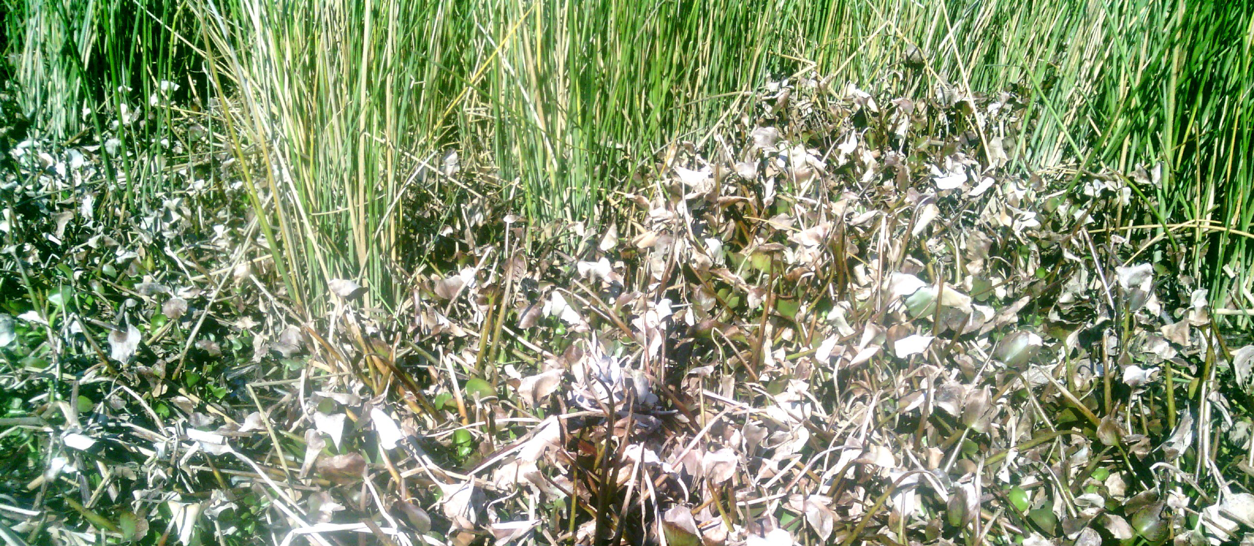
Emergent Vegetation (EMR)Cat tail (Typha spp.), common reed (Phragmites australis), giant reed (Arundo donax), and tule (Schoenoplectus spp.)
Water HyacinthWater Hyacinth (Eichhornia crassipes)
Water PrimroseWater Primrose (Ludwigia spp.)
RiparianShrubs and trees in the area including willow species (Salix spp.)
Submerged Aquatic Vegetation (SAV)Numerous species; dominant ones include: Brazillian waterweed (Egeria densa), coontail (Ceratophyllum demersum), and watermilfoil (Myriophyllum spicatum) [37]
WaterWater
Other VegetationSpecies or cover not observed in the UAV study region including pennywort (Hydrocotyle spp.) and mosquito fern (Azolla spp.)
Non-Photosynthetic Vegetation (NPV)Senescent or dead vegetation
Table 2. Sensor and Platform Specifications.
HyMapNano-Hyperspec
Typewhiskbroompushbroom
Spectral Range450–2480 nm400–1000 nm
Number of bands128270
Spectral Resolution15–18 nm2.2 nm
Signal to Noise>500:1>15:1 (1000 nm) < 140:1 (550 nm)
Spatial Resolution *1.7 m0.051 m
Swath Width (FOV°)61.315.85
Operational Altitude>458 m **<122 m ***
Platform1975 Rockwell International 500-SDJI-M600P
* Note: spatial resolution is not only dependent on the sensor but also the flight altitude. ** Typical lowest safe altitude according to FAA. *** Maximum altitude for UAV without FAA approval.
Table 3. HyMap and Nano Classification Performance by Year.
YearSensorClassification ModelOverall AccuracyKappa Coefficient
2019NanoRFC 1530.9410.926
2019HyMapCSTARS0.8570.830
2018HyMapCSTARS0.9080.900
The training/test split for the selected Nano model was 65/35%. The decrease in CSTARS classification performance in 2019 was due to a lower quantity of labeled reference data for some classes in 2019.
Table 4. Class area coverage for the HyMap, Nano, nearest neighbor (NN) resampled Nano, and moving window resampled Nano maps.
ClassHyMap Area (m2)Nano Area (m2)Nano NN Resampled Area (m2)Nano MW Resampled Area (m2)
Bare ground858.3930.4956.61002.8
EMR19,097.112,077.114,68711,666.9
Water Hyacinth0.001589.4124.3145
Water Primrose349.71616.5317.917.3
Riparian14,952.912,58311,45613,146.6
SAV698890238594.98869.4
Water41,269.244,822.942,422.341,257.6
Other679.2000
NPV13,577.216,989.320,883.121,177.9
Table 5. Mean agreement and standard deviation between HyMap pixel and Nano pixels contained within by class.
ClassMean AgreementStandard Deviation
Bare Ground31.92%3.15%
Emergent30.82%28.77%.
Water HyacinthNANA
Water Primrose4.17%6.63%
Riparian62.62%36.97%
SAV47.64%43.12%
Water88.50%28.67%
NPV69.17%32.71%
Table 6. Errors of omission and commission were calculated from the confusion matrix for the upscaled Nano maps using HyMap as a reference. Note: Absent classes had no occurrences in one of the maps.
TypeClassResampledMoving Window
Overall Error 29.18%28.12%
Omission ErrorBare ground63.97%61.51%
EMR58.95%58.62%
Water Primrose100.00%100.00%
Riparian Shrub32.56%30.04%
SAV50.79%50.52%
Water11.54%11.13%
NPV18.55%15.96%
Commission ErrorBare ground67.72%67.72%
EMR32.65%32.65%
Water Primrose100.00%100.00%
Riparian Shrub21.10%21.10%
SAV61.19%61.19%
Water11.34%11.34%
NPV46.38%46.38%
Table 7. Nano and HyMap Operational Information and Cost Estimates.
SensorArea Covered (hectares)Flight Time Estimate (hrs)Approximate Data Volume (GB)Approximate Deployment Costs
HyMap74,123.4216700$150,000
Nano—This Study10.531600$62,780
Nano—Entire Delta74,123.4270402,111,880$865,014
Publisher’s Note: MDPI stays neutral with regard to jurisdictional claims in published maps and institutional affiliations.

