Article

Data Assimilation for Rainfall-Runoff Prediction Based on Coupled Atmospheric-Hydrologic Systems with Variable Complexity

1
State Key Laboratory of Simulation and Regulation of Water Cycle in River Basin, China Institute of Water Resources and Hydropower Research, Beijing 100038, China
2
College of Hydrology and Water Resources, Hohai University, Nanjing 210098, China
*
Author to whom correspondence should be addressed.
Remote Sens. 2021, 13(4), 595; https://doi.org/10.3390/rs13040595
Submission received: 31 December 2020 / Revised: 30 January 2021 / Accepted: 3 February 2021 / Published: 7 February 2021

Abstract

:
The data assimilation technique is an effective method for reducing initial condition errors in numerical weather prediction (NWP) models. This paper evaluated the potential of the weather research and forecasting (WRF) model and its three-dimensional data assimilation (3DVar) module in improving the accuracy of rainfall-runoff prediction through coupled atmospheric-hydrologic systems. The WRF model with the assimilation of radar reflectivity and conventional surface and upper-air observations provided the improved initial and boundary conditions for the hydrological process; subsequently, three atmospheric-hydrological systems with variable complexity were established by coupling WRF with a lumped, a grid-based Hebei model, and the WRF-Hydro modeling system. Four storm events with different spatial and temporal rainfall distribution from mountainous catchments of northern China were chosen as the study objects. The assimilation results showed a general improvement in the accuracy of rainfall accumulation, with low root mean square error and high correlation coefficients compared to the results without assimilation. The coupled atmospheric-hydrologic systems also provide more accurate flood forecasts, which depend upon the complexity of the coupled hydrological models. The grid-based Hebei system provided the most stable forecasts regardless of whether homogeneous or inhomogeneous rainfall was considered. Flood peaks before assimilation were underestimated more in the lumped Hebei model relative to the other coupling systems considered, and the model seems more applicable for homogeneous temporal and spatial events. WRF-Hydro did not exhibit desirable predictions of rapid flood process recession. This may reflect increasing infiltration due to the interaction of atmospheric and land surface hydrology at each integration, resulting in mismatched solutions for local runoff generation and confluence.

Graphical Abstract

1. Introduction

The last decades have witnessed significant changes in climate and hydrological conditions. The increased frequency of extreme storm floods has led to major risks of damage due to weather-related hazards. Forecasting of such high-intensity floods on a shorter time scale has immense benefits such as saving lives, protecting economic assets, and improving quality of life [1,2,3]. For mesoscale mountain areas along the Daqing River of northern China, steep slopes, combined with high intensity and short duration convective rainfall, substantially shorten hydrological lead times. In addition, due to the lack of high-resolution and dense observations, the “throughfall” observed by rain gauges cannot reflect the realistic rainfall distribution in space and time, thus the accuracy of forecasting is limited by the layout of the rain gauge network. For processes of runoff and routing, different dependent processes are added and derived within models including soil infiltration, overland transport, and channel routing, which result in the complexities and uncertainties in deducing the generation mechanisms of flash floods. In this study, we selected two upstream mountainous catchments along the Daqing River in which there is an urgent need for accurate flood prediction to prevent and reduce risks facing the construction of the downstream including Xiong’an New Area.
Although recent advances have improved rainfall forecasting [4], several challenges remain. One such challenge is the reproduction of the magnitude and the disturbance patterns of rainfall that can assimilate suitable observations into numerical weather prediction (NWP) models [3]. Rainfall is among the variables generated with the greater errors in NWP models, while it plays an important role in forecasting the atmospheric-hydrological processes for its influence on the time and scale of floods [5,6]. There are three main sources of error in rainfall prediction: the initial conditions, the lateral boundary conditions, and the physical approximations in the model equations. Data assimilation allows atmospheric information to be extracted from multiple data sources, thereby improving the reliability of coarse resolution data and the complexity of atmospheric motion, reducing the initial and lateral boundary errors [7,8]. Routray et al. [9] found that weather research forecasting (WRF) can be used to assimilate observations from different sources and contribute to a better understanding of mesoscale rainfall convective activity within the Indian monsoon region. Kumar and Varma [10] further explored a short duration intense rainfall event in India, demonstrating the potential of WRF to adapt to rainfall forecast accuracy. Fierro et al. [11] conducted a data assimilation study in the eastern part of the USA that showed that WRF, in conjunction with data assimilation, could significantly improve models of local short-term rainfall processes. Although data assimilation can help NWP models to more accurately capture rainfall and enable rainfall-runoff conversion by constructing an atmospheric-hydrological model system, its potential to further improve flood forecasting has not been fully investigated.
A reliable atmospheric-hydrological model system is required to improve rainfall predictions and hydrological forecasts for early flood hazard mitigation [12]. A promising method is the coupling of hydrological models to a regional model such as NWP, in order to rapidly obtain high-resolution rainfall and flood forecasting data. In [13,14,15], Lin et al. and Lu et al. discussed the implementation and improvement of the Canadian regional mesoscale compressible community mode (MC2) rainfall forecasting in the Huaihe Basin of southern China, concentrating on the Huaihe sub-basin coupled to the Xinanjiang hydrological model. Wu et al. [16] further explored MC2 and the multiple linear regression integrated forecast and found that high-resolution rainfall distributions were problematic at finer temporal and spatial scales, requiring data assimilation or sub-grid-scale parameterization. Yucel et al. [4] and Moser et al. [17] tested WRF data assimilation as the input for flood forecasting in the Black Sea and Iowa, respectively, both finding an enhancement in the accuracy of flood warnings.
With regard to the selection of coupled models, it is subject to a diversity of laws and non-universality, which makes it difficult to accurately express physical movement processes. The hydrological model has a more comprehensive physical foundation including lumped, grid-based, and fully distributed setups [18,19]. Not only the above physically-based models are used, but machine learning models are also widely applied in rainfall-runoff forecasting (i.e., artificial neural networks (ANNs) [20], support vector machines (SVM) [21], and the recent emergence of theory-guided data science (TGDS) [22,23]. For flood forecasting, which is affected by the discretization construction method, different construction expressions determine variations between heterogeneity analysis and model calculation structure, and further influence the accuracy of physical expressions in the prediction processes of the hydrological model [24,25,26]. To analyze the scale of hydrological processes, large-scale studies are still the mainstay. During the last ten years, a focus has been made on downscaling and modeling through appropriate discrete methods [27]. The development of models with high prediction accuracy and computational efficiency is a key issue for basin-scale flood forecasting. Liu et al. [28] conducted coupled lumped hydrological modeling and WRF flood forecasting on a 135.2 km2 catchment with a 10 km resolution; Li et al. [29] used the rainfall of a 20 km WRF output to drive the distributed Luxihe model, extending the forecast period of flood forecast in the Liujiang catchment (58,270 km2). Rogelis [30] compared the flow results of different resolution data (minimum resolution 1.67 km) driven by WRF on a 380 km2 catchment driving different lumped hydrological models. Previous studies have mostly focused on humid regions; consequently, runoff methods are mostly based on saturation excess, and limited discussion of the appropriate construction of atmospheric-hydrological model systems have been conducted for semi-humid and semi-arid areas.
The coupling system can also integrate land surface models (LSM) with hydrological models. Most LSM and hydrological models incorporate the same descriptions of water balance, albeit with different aims [31,32]. LSM evolves from land-atmosphere coupling models with the purpose of solving the surface energy balance equation and providing the necessary lower boundary conditions for the atmosphere [31,33]. Inversely, hydrological models focus less on radiation and more on hydrological changes (i.e., the lateral route of water along land surfaces). Such models are the most complicated among the current coupling systems due to their complex structure and the sensitive parameters to be determined in the relevant physical processes as well as hard parameters (fixed parameters written directly into the source code during the compilation of the model).
Limited research has been undertaken to model atmospheric-hydrological processes in semi-humid and semi-arid regions of northern China. Consequently, there is a lack of effective atmospheric-hydrological coupling forecasting systems for this region. Herein, we used WRF models, three-dimensional variational (3DVar) data assimilation modules coupled to three model sets of varying complexity to construct the required model systems. To test the influence of various levels of complexity, three types models were selected, namely the lumped Hebei model, the grid-based Hebei model, and the WRF-Hydro model. These models were both standalone and coupled with the WRF model and three-dimensional variational (3DVar) data assimilation module. Four typical storm flood events with different spatial and temporal rainfall distributions, all of which occur in the upper catchment of the Daqing catchment, were explored before and after data assimilation. The purpose of this study was to investigate the impact of data assimilation on forecasting different types of rainfall-runoff events after coupling with variable hydrological structures. It should be noted that the atmospheric-hydrologic coupling in this study refers to “one-way” coupling of the three standalone hydrological model structures with the WRF and 3DVar data assimilation module, which means that the hydrological models are driven by the WRF and 3DVar outputs without feedback to the atmospheric modeling processes. The results obtained in this way can simply reflect the direct effects of data assimilation on rainfall as well as runoff forecasts.
There were four basic questions we aimed to explore:
  • What are the differences in the improvement of rainfall before and after data assimilation for the storm events with different spatial and temporal distributions in semi-humid areas of northern China?
  • What are the corresponding runoff effects of different coupling systems on the improved rainfall from WRF and its assimilation mode?
  • What differences exist between the runoff processes modeled by the coupled systems of different complexity before and after assimilation?
  • How does the complexity of the hydrological structure affect the transmission of rainfall improvement from data assimilation to runoff?

2. Study Area and Events

2.1. Study Area

We studied two mountainous catchments of the Daqing River (i.e., Fuping (2210 km2) and Zijingguan (1760 km2)). Two catchments lie along the upper reach of the Shazhi River on the south branch and the upper reach of the Juma River on the north branch, respectively (Figure 1). Low vegetation coverage, bare hills, mountains, and thin soil layers cause uneven infiltration capacity distribution across the study areas, and the surface often features extra-infiltration flow, which means surface flow occurs when the intensity of infiltration exceeds the intensity of precipitation. Rainfall occurs primarily during the flood season from late May to early September. The combined effects of the western Pacific subtropical high, the westerly cold vortex, and the western Taihang Mountain uplift influence the heavy convective rainfall that prevails in the region. Additionally, due to steep terrain, it is easy to form high intensity, short duration floods with a large peak flow. These floods cause damage in the region. According to statistics of torrential rain and flood data from 1958 to 2015 in both catchments, floods that occurred more than once a decade occurred five times in Fuping and six times in Zijingguan, with increasing frequency in extreme events in recent years.

2.2. Storm Events

Four storm events in the Fuping and Zijingguan catchments were screened. The events were divided according to their spatial and temporal distribution. In comparison to the southern part of China, it is difficult to find absolute homogeneous rainfall events in northern China, either in spatial or temporal dimensions. Herein, we calculated the storm events’ coefficient of variance (Cv) values to indicate the relative response to the spatio-temporal homogeneousness of the flood events [34]. Cv values were calculated as follows:
C v =   i = 1 N ( x i x ¯ 1 ) 2 N
where x ¯ is the average of xi. When calculating Cv in the temporal dimension, xi is the catchment areal rainfall at the ith hour and N is the total number of hours of the storm event. In this case, time Cv represents the temporal deviation of the catchment areal rainfall at each time step. When calculating Cv in the spatial dimension, xi is the 24 h rainfall accumulation at the ith gauge and N is the number of rain gauges. In this case, the Cv value reflects the spatial deviation of the rainfall accumulation at each rain gauge.
The results are shown in Table 1, where larger Cv values represent a more uneven spatio-temporal distribution. Based on this criterion, the spatio-temporal consistency of the rainfall-runoff events listed in Table 1 were classified. Events 1 and 2 had relatively uniform spatial and temporal distributions, whereas Events 3 and 4 featured rainfall with uneven spatial and temporal distributions. As shown in Figure 2, the rainfall-runoff events had a flood recession time with different lengths, so we used a 72-h time window for Event 1 and Event 2, a 60-h time window for Event 3, while for Event 4, a 36-h time window was adopted. Different time windows were used to calculate the statistics when evaluating the forecasting results. Event 4 occurred on 21 July 2012, bringing the largest flood disaster in 60 years to Beijing and the Daqing River. The rainfall at the largest monitoring point corresponded to an event that occurred once in more than 500 years. In the Zijingguan catchment, its 24 h maximum single station cumulative rainfall was 355 mm, and the maximum flow at the outlet reached 2580.0 m3/s. Figure 2 and Table 1 show other rainfall and flood characteristics.

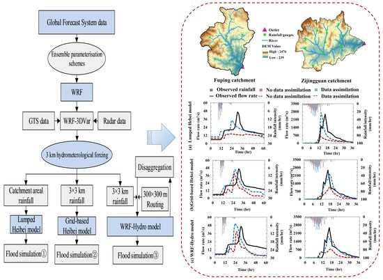
3. Three Atmospheric–Hydrologic Coupled Systems

3.1. The Numerical Weather Prediction (NWP) Model

The mesoscale NWP model has limited skill in convective precipitation forecast, even in the WRF model. One of the considerable reasons for the poor performance is due to its nonlinear and chaotic nature, since solving quasistationary meso-β and meso-γ processes is complicated [35,36], and the power spectrum of the turbulence in convective motion has a resolution of a few kilometers [37,38]. 3DVar data assimilation could merge the fine rainfall information into the modeling system to obtain accurate high-precision rainfall data. The following are detailed descriptions of the WRF model configurations and the 3DVar data assimilation techniques used in this study.

3.1.1. Weather Research Forecasting (WRF) Model Configurations

As a next-generation mesoscale forecasting model and data assimilation system, the simulated scale used in the WRF spans tens of meters to thousands of kilometers, and is mainly used to enhance understanding and forecasting of mesoscale weather, assist operational forecasting, and improve atmospheric research. Detailed descriptions of specific WRF model settings are shown in Table 2 and Figure 1. The inner research area includes the Taihang Mountains, Bohai Sea, and major cities in Beijing, Tianjin, and Hebei. A warm-up time period is necessary for both WRF and WRF-Hydro. A seven-day length warm-up time period was set to generate the restart file, which serves mainly as the starting condition for WRF, and was also used to provide the initial soil moisture condition for WRF-Hydro to generate more realistic runoff. The WRF has an output time step of 1 h and an integration step of 6 s. Global Forecast System (GFS) data in each 6 h window was to provide the initial side boundary and atmospheric background conditions.
The parameterization scheme chosen can affect the mode of operation of the WRF; different parameterization schemes have different emphases on physical processes. The diversity of parameterization schemes and the corresponding differences in rainfall events in specific regions result in difficulties inherent to the accurate simulation of spatial and temporal rainfall distributions and cumulative rainfall. For the four rainfall processes in this study, we chose the optimal physical parameterization based on the relevant experimental research on the selection of sensitive parameterization schemes for ensemble rainfall forecasting (more details can be found in Tian et al. [39,40]). The microphysical parameterization schemes chosen for our forecasts included Purdue-Lin (Lin) [41] and WRF Single-Moment 6 (WSM6) [42]; the cumulus convection schemes included the Kain-Fritsch (KF) [43] and Grell-Devenyi (GD) [44] ensembles; and the planetary boundary layer schemes included the Yonsei University (YSU) [42] and Mellor-Yamada-Janjic (MYJ) [45] schemes. The specific parameterization details of the four studied storms are shown in Table 3. It should be noted that the cumulus parameterization was not used in the innermost domain, where the convective rainfall generation was assumed to be explicitly resolved.

3.1.2. Data Assimilation with WRF-3DVar

3D variational assimilation has numerous advantages, for example, that the objective function contains physical processes and utilizes the model itself as a dynamic constraint (i.e., it can efficiently represent complex nonlinear constraint relationships). The objective function of WRF-3DVar assimilation can be expressed as follows:
J ( X ) = 1 2 ( X X b ) T B 1 ( X X b ) + 1 2 ( H ( X ) Y 0 ) T R 1 ( H ( X ) Y 0 )
where X is a parameter reflecting the atmosphere and surface conditions; Xb is the background field at the time of change; B is the corresponding background field error covariance matrix; and H is the observation function containing X variables. H can change the variables in the atmospheric model from model space projected into the observation space. Y0 represents the assimilated observation vector and R is the error covariance matrix from observation.
Global Telecommunications System (GTS) data and Doppler radar data were used as the assimilation data in this study. In previous studies, we have demonstrated that the assimilation of radar reflectivity can improve local rainfall processes, especially for data <500 m, and can thus improve the reliability of assimilation information for forecasting systems [46,47]. Taking into account the spatial resolution of data from different sources and maintaining the stability of the atmospheric motion, we chose to assimilate <500 m radar reflectivity data in the inner domain (Dom2) and GTS data in the outer domain (Dom1). This assimilation method was supported by multi-source data assimilation experiments carried out in the same study area [47].
GTS data are a collection of traditional ground and upper air meteorological data including barometric pressure, wind direction and velocity, temperature, and humidity. GTS data have wide coverage in both the vertical and horizontal directions. These data are updated at 6 h intervals and are therefore widely used in large-scale atmospheric studies. GTS data provided by the National Center for Atmospheric Research (NCAR) were assimilated for the outer domain, sourced from sounders, ground-based weather stations, pilot balloons, and aircraft observations. An observation preprocessor with defined observation error covariance was employed to ensure quality control of the GTS data prior to assimilation, and a default U.S. Air Force (AFWA) OBS error file was also used for processing the GTS data and identifying instrumental and sensor errors.
The forecasting radar site of the Shijiazhuang s-band Doppler weather radar and specific coverage is shown in Figure 1. Its reflectance spatial resolution was 1 km × 1° with a scan radius of 250 km (i.e., it covered both the Fuping and Zijingguan catchments). The radar completed a cycle every 6 min at nine different scan elevation angles (0.5°, 1.5°, 2.4°, 3.4°, 4.3°, 6.0°, 9.9°, 14.6°, and 19.5°). Raw data for the radar were obtained from the National Meteorological Administration of China and, following quality control, the radar reflectivity was programmed to conform to the WRF-3DVar data format.
The absorption of radar reflectivity data by the WRF-3DVar module presupposes that the total water mixing ratio is used as a control variable and that a warm rainfall process is simultaneously introduced into the assimilation module. Assuming a Marshall-Palmer raindrop size distribution and no ice relative reflectivity effect, the following equation can be derived for radar reflectivity Z by introducing a rainwater mixing ratio qr, in which ρ is the density of air in kg m−3:
Z = 43.1 + 17.5 log ( ρ q r )
For the four storm events, we selected a uniform 24 h time window that completely described the entire process of rainfall. The duration of the WRF is required to cover the start and end of the rainfall time window; therefore, the assimilation data started to be merged 6 h before the storm events, then assimilated every 6 h until five assimilation cycles were completed, for a total running duration of 36 h (6 × 6 h). Figure 3 presents a schematic diagram of the assimilation using Event 4 for further explanation. As illustrated in Figure 3, there was a seven day warm-up time period (indicated with a dashed line) and a 6 h spin-up time period (indicated with dotted lines) for WRF, and run1 presents the initial WRF run with no data assimilation. Data assimilation started at 00:00 on 21 July 2012 and, subsequently, run2, run3, run4, run5, and run6 were executed at 6 h intervals (i.e., at 00:00, 06:00, 12:00, and 18:00 on 21 July 2012 and 00:00 on 22 July 2012, respectively). The first output file generated in the previous run was used to provide the initial and lateral boundary conditions for subsequent runs and was treated as a benchmark reflecting improvements in rainfall simulation after data assimilation.

3.2. Hydrological Models with Differing Complexity

3.2.1. The Lumped Hebei Model

The lumped Hebei model was developed based on rainfall-runoff mechanisms identified in semi-humid and semi-arid catchments in northern China and has been applied to real-time flood forecasting in Hebei Province. The model comprehensively considers the two inflow mechanisms of infiltration excess and saturation excess (shown in Figure 4). W’ and WMM represent the point storage capacity and the storage capacity of the maximum point in catchments. γ and λ are the proportion of the infiltration capability beyond a certain value and the proportion of runoff generation in the catchment. When rainfall intensity was greater than infiltration intensity during the studied period, surface runoff occurs, whereupon continuous infiltration supplements the soil moisture deficiency until the system reaches the point soil water capacity, generating underground runoff. The model divides soil into two layers, in which soil depth should be determined according to the conditions of the catchment. The volume of infiltration (ft), surface (rs), and groundwater (rg) can be calculated using Equations (2)–(4) as follows:
f t = i = 1 t f ¯ i = ( i i ( 1 + n ) ( 1 + n ) f m n ) e u m + f c
r s = p t f t
where p t (mm/h) is the rainfall rate during the ith hour and f ¯ i (mm/h) is the ith hour empirical infiltration rate computed by a variant of Horton equation; m (mm) is the surface soil moisture; and u is an index accounting for the decreasing infiltration rate with increasing soil moisture. fc (mm/h) and fm (mm/h) are the stable infiltration rate and the infiltration capacity, respectively. It follows that:
r g = { f t + p a e t w m p a + f t w m f t + p a e t w m + w m ( 1 f t + p a w m ) 1 + b p a + f t < w m
where et is the evaporation volume; pa (mm) represents the rainfall influenced; wm (mm) is the average storage capacity; and b is a coefficient of the water storage capacity curve.

3.2.2. The Grid-Based Hebei Model

The grid-based Hebei model retains the runoff generation concepts behind the lumped Hebei model. Furthermore, it develops terrain index T [48,49] to obtain a grid-type representation of soil moisture storage and infiltration capacity. T = ln(α/tanβ), where α and β are the grid scale and shape parameters, respectively. The value of T in the Fuping and Zijingguan catchments were statistically analyzed. Experimentation demonstrated that the cumulative distribution curves of T values between different regions are always similar [50]. The T values of different grids in the same region can be expressed by a parabolic empirical formula. Hence, the soil water storage capacity and infiltration capacity of different grids can be determined as followed:
W i W M M = exp { [ ln ( T i T min + 1 ) α ] β }
f i f m = { 1 [ 1 exp [ 1 α [ ln ( T i T min + 1 ) ] β ] b } 1 / n
where i is a certain grid cell, and Ti and Wi (mm) are the corresponding moisture storage capacity and terrain index of the ith grid. Tmin is the minimum value of the grid terrain index. In a non-channel grid, surface runoff outflow q s o = q s i + q s , where qs is the grid surface runoff. qs occurs when the rainfall intensity exceeds fm. qsi denotes the runoff values generated via the surrounding upstream grid. Similarly, the generated groundwater runoff from upstream grid (i.e., qg, is transmitted to the groundwater runoff outflow according to qgo, q g o = q g i · ( 1 μ ) + q g , where μ is the ratio coefficient). The grid-based Hebei model adopts a simplified form of the Saint Venant equations for confluence calculation. Due to perennial channel water shortage and substantial channel seepage in the study area, an additional Horton infiltration equation was considered in the grid-based Hebei model [50].

3.2.3. The WRF-Hydro Modeling System

The open-code WRF-Hydro model is a multi-core parallel, multi-physics, multiscale, fully distributed hydraulic model. It can be operated only with meteorological data or coupled with the WRF model to constitute the atmospheric-hydrological model system. Its multiscale 3D land surface hydrological simulation mode can improve the one-dimensional vertical generalization of water transport using the original LSM Noah and Noah-MP. WRF-Hydro can use additional modules to achieve lateral flow exchange between the surface and subsurface, thereby improving upon the “column-only” one-dimensional vertical structure. It uses a disaggregation-aggregation solution module between the land model and terrain routing grid, which enables convergence processes occurring at a smaller resolution. WRF-Hydro can set the variables of the scale factor including soil moisture and excess infiltration into the fine grid values.
Noah or Noah-MP LSM are connected to WRF-Hydro to calculate water and heat flux exchange processes. In Noah-MP, a column cylinder structure is used to substitute soil layers into thicknesses, from top to bottom, of 0–10 cm, 10–40 cm, 40–100 cm, and 100–200 cm. The inputs required by WRF-Hydro include meteorological forcing data such as rainfall, air temperature, relative air humidity, surface pressure, wind speed, downward longwave radiation, and downward solar radiation. Gochis and Chen [51] described a sub-grid, spatially weighted disaggregation-aggregation solution to coordinate the land model and terrain routing grid in WRF-Hydro. Its runoff generation method uses a simple water balance (SWB) [52]. Similar to the Hebei model, when the rainfall capacity exceeds the infiltration capacity, a surface infiltration excess occurs in the top soil layer and the corresponding change in surface water depth h (m) is:
h t = p e t { 1 [ k = 1 4 Z i ( δ s δ k ) ] [ 1 exp ( S R d t R f d Δ t 86400 ) ] p e + [ k = 1 4 Z i ( δ s δ k ) ] [ 1 exp ( S R d t R f d Δ t 86400 ) ] }
where h (m) refers to the change in surface water depth; Δt (s) is the model time step; k is the integer number of the soil layer (i.e., 1–4), Zk (m) and δ k (m3m−3) are the depth and grid soil moisture of the kth soil layer; δ s (m3m−3) is the maximum soil moisture content; S is a coefficient given by Richards’ equation to regulate runoff infiltration; and Rdt and Rfd represent the tunable surface infiltration coefficient and saturated hydraulic conductivity, respectively.
Subsurface routing followed the approach of Wigmosta and Lettenmaier [53] by using a quasi-3D flow taking into account topography, saturated soil depth, and saturated hydraulic conductivity with soil depth. Overland routing is a fully unsteady finite-difference and diffuse wave approach, implemented as described in Downer et al. [54]. River routing is similar to the overland case, using an explicit, one-dimensional, variable time-step diffusion wave equation. Details of specific rainfall-runoff processes can be obtained from the official user guide [55].

3.3. Establishment of Three Coupled Atmospheric-Hydrological Systems

Figure 5 shows a flood prediction diagram for coupled systems comprising three types of hydrological models, WRF models, and WRF-3DVar data assimilation modules. Rainfall in the WRF model was enhanced through optimal parameter scenarios and assimilation. GTS data and radar reflectivity were assimilated every 6 h to generate 3 km grid data in the inner layer Dom2. To eliminate the deviation of rainfall, for each storm, the best performance in the assimilated rainfall ensemble was selected as the forecast forcing data. Subsequently, predicted rainfall was converted into discharges using the aforementioned three models, with parameters calibrated using 17 historical rainfall-runoff events from the two studied catchments since the 1980s. For the calibration of WRF-Hydro, previous parameter sensitivity analysis in the study area noted several key parameters that can cause large fluctuations in flooding prediction including the runoff infiltration parameter (REFKDT), the channel Manning roughness parameter (MannN), the surface retention depth scaling parameter (RETDEPRTFAC), and the overland flow roughness scaling parameter (OVROUGHRTFAC). To evaluate the impact of data assimilation on the obtained runoff, WRF outputs under the selected optimal parameterization scheme were also used to drive the model for runoff forecasting; the results of the three systems before and after data assimilation were compared as described below.
The three coupling systems tested showed three types of rainfall input at different resolutions. The lumped model gives selected grid-averaged rainfall data across the sub-basins, whereas the grid-based Hebei model and WRF-Hydro directly pass the grid coordinates to locate forcing data. The former has a rainfall resolution of 3 km, and the latter has a grid division factor of 10 to allow further downscaling from the WRF assimilation data to 300 m of routing data.
The Nash efficiency coefficient (NSE), relative flood peak (Rp), and relative flood volume (Rv) were used to analyze the flow discharge forecasts as follows:
N S E = 1 i = 1 n ( q i q i ) 2 i = 1 n ( q i q ¯ ) 2
R p = ( q p q p ) / q p
R v = ( r v r v ) / r v
where i is the time step; n is the total i of flood processes; q i , q i , and q ¯ are the simulated, observed, and averaged flood discharge, respectively; q p and q p are the simulated and observed discharge; respectively; and r v and r v are the simulated and observed flood volumes, respectively.

4. Results

The forecasting results for the three coupled systems before and after data assimilation for the four studied rainfall-runoff events are shown in Figure 6. In each single subfigure, the black bars and black solid curve indicate observed rainfall and runoff, respectively. Red and blue bars and curves indicate rainfall and runoff before and after data assimilation. For the studied coupling systems, assimilation had different degrees of enhancement on rainfall and runoff. The following analyses were conducted separately for data assimilation on the rainfall, runoff, and model systems.

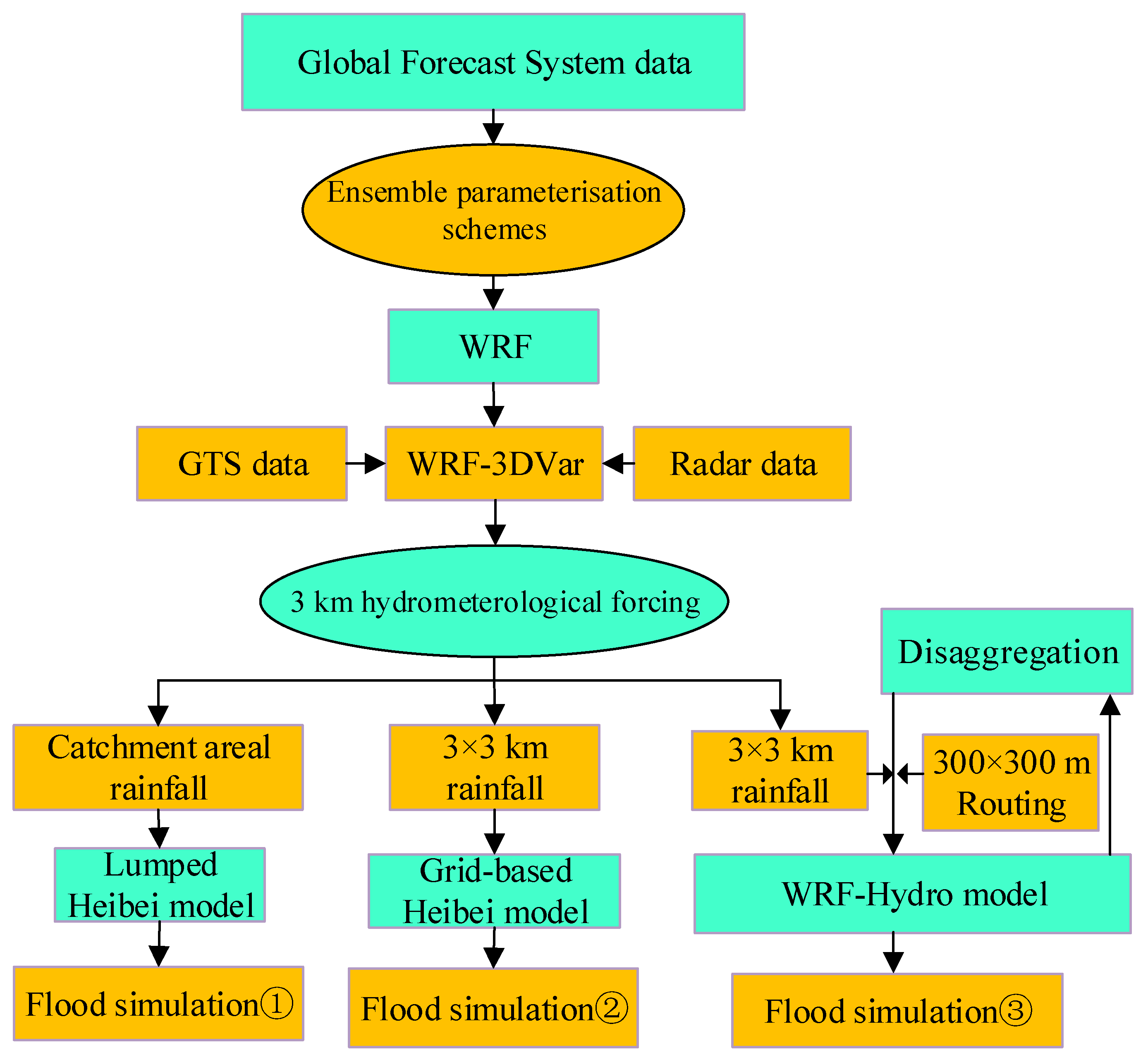
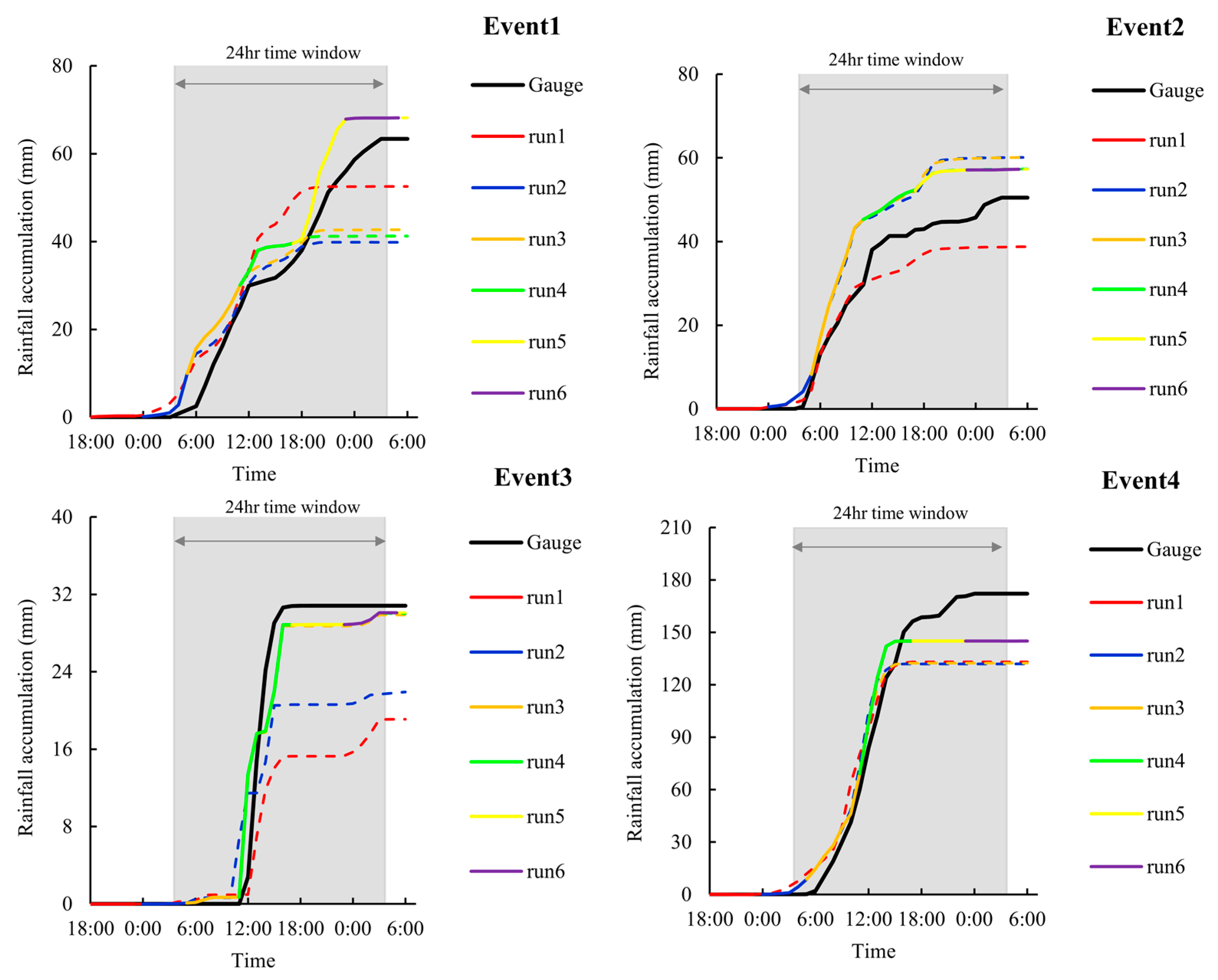
4.1. Effect of Data Assimilation on Rainfall Prediction

Figure 7 shows the cumulative precipitation variation over the simulated period caused by the cycling assimilation processes. The black solid curve represents the observed precipitation, while the other colors represent different assimilation periods. As above-mentioned, run1 was a non-assimilated precipitation process. Under conditions of data assimilation every 6 h, it was found that the cumulative rainfall gradually approached the observed values by the end of run6. For Event 2 and Event 3, the performance of run2 and run3 relative to run1 was impressive. For Event 1, run4 and run5 changed and improved the temporal distribution of precipitation within a few hours after data assimilation, while run2 and run3 seemed to show slightly worse results than run1, if no further assimilation took place. Generally, forecasts of cycling data assimilation after five cycles were largely stable for all events and the final curve integrated by the data assimilation runs (run2 to run6) was enhanced relative to the original run (run1). In addition to showing good performance for selected typical precipitation events, the cycling data assimilation gradually improved the temporal variability.
Table 4 presents further statistics regarding the performance of data assimilation in improving cumulative rainfall. This shows that precipitation significantly increased compared to the period of no data assimilation. Overall, the relative error (RE) before and after assimilation was reduced by 0.26; Event 3 errors resulted in the most significant change, with a reduction in deviation of 0.342, while Event 4 rainfall increased most after assimilation by 19.76 mm.
The normalized Taylor diagrams of cumulative rainfall (in which the horizontal and vertical coordinates are normalized by dividing by the standard deviation (SD) of the observed series) before and after assimilation are shown in Figure 8. The variations of the assimilated results were closer to the actual observations. The correlation coefficients (CC) for both cumulative rainfall before and after assimilation were above 0.9 and the correlation coefficient and root mean square error (RMSE) after data assimilation showed a significant improvement compared to the corresponding values before assimilation, especially for Event 1, in which the CC increased from 0.93 to 0.99. In the case of Event 3, a decrease in CC from 0.98 to 0.96 occurred after assimilation; a similar trend was noted during Event 4. The previous calculations of the temporal Cv values for precipitation events showed that the two precipitation events were more heterogeneous in time and space than Event 1 and Event 2. In Event 3, for example, the temporal Cv value of 2.3925 was much higher than that of Event 1 (0.6011). This may explain the increased bias in assimilation, since the improved effectiveness of the rainfall forecast after assimilation is determined by the amount of effective information contained in the data. It is clearly easier for radar and GTS to capture data during periods of rainfall that are homogeneously distributed in space and time.
The above results demonstrate that WRF-3DVar effectively improved the consistency of simulated precipitation. Specifically, cycling assimilations of radar reflectivity and GTS data in the study area were able to improve both initial and lateral boundary conditions, providing a basis for future research into the accurate modeling of atmospheric-hydrological systems.

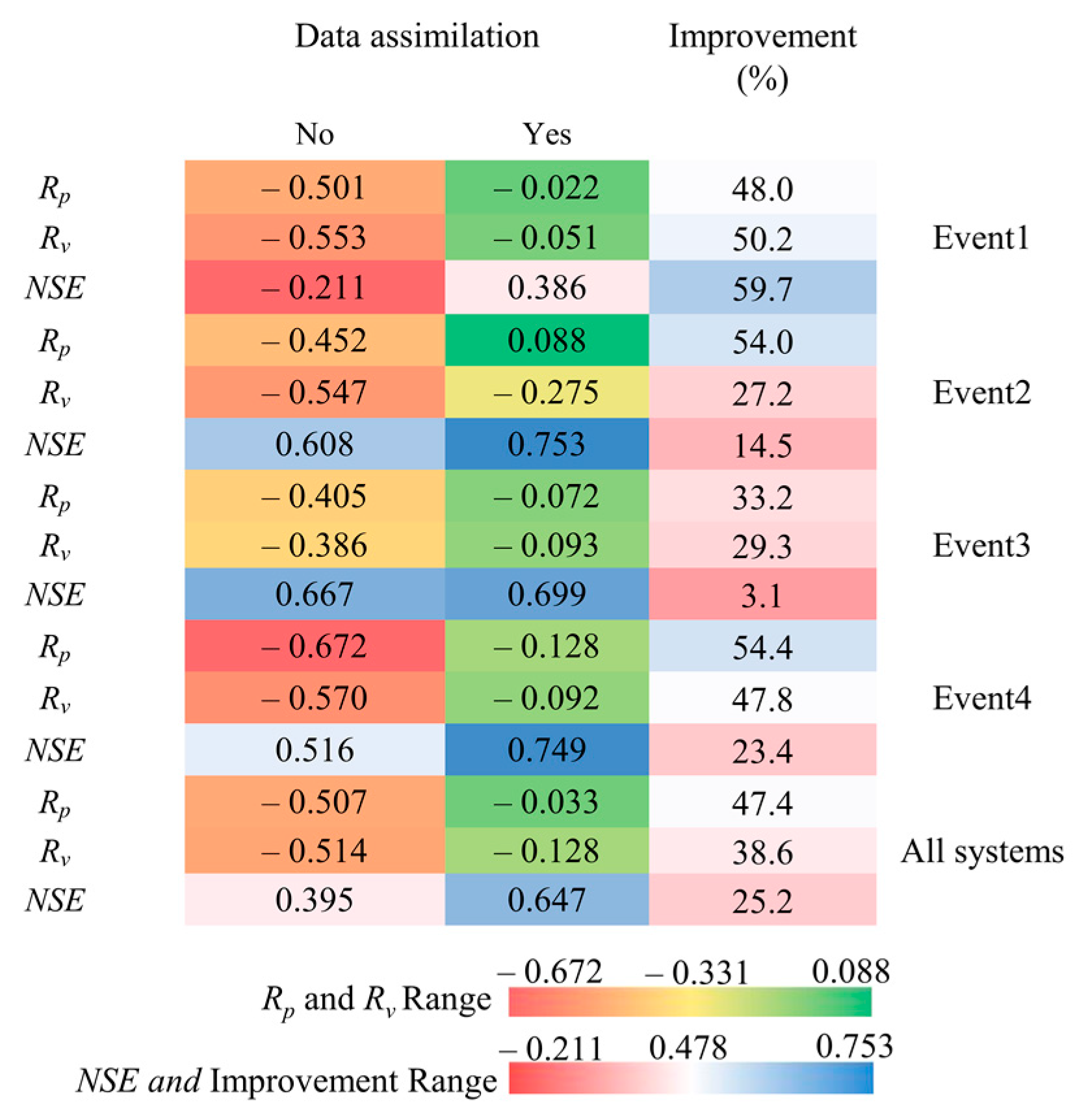
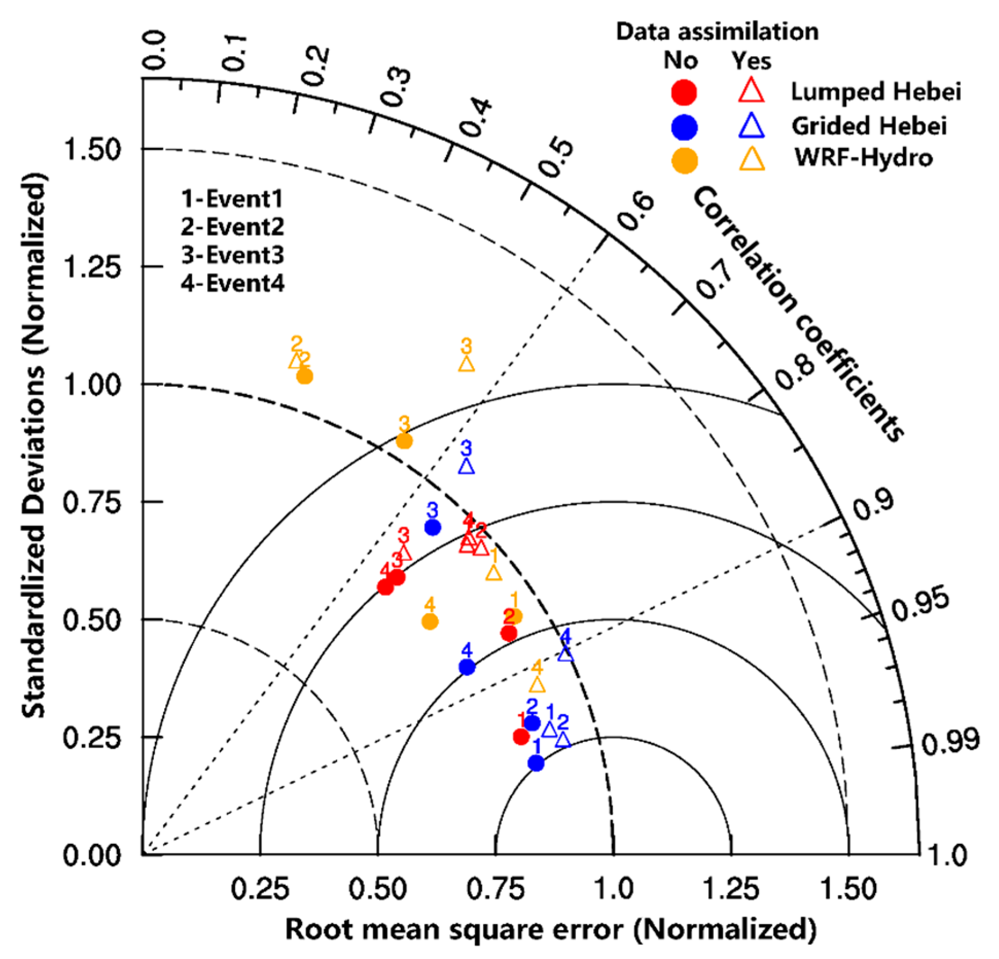
4.2. Effect of Data Assimilation on Runoff Prediction

In addition to the above analyses of the precipitation process, the performance of the data assimilation on the runoff process was also of interest. We found that runoff forecasts were relatively effective when data assimilation was used. For example, the coupling system from the lumped model simulated Event 2 had significant improvements in flood peak after assimilation (Figure 6).
The evaluation of the NSE, Rv, and Rp indices heat map among the flood processes for the four studied events are given in Figure 9. To evaluate the effects of data assimilation on runoff prediction, the indices of events were averaged from the results of the three coupled systems with different complexities. Figure 9 also shows the degree of improvement of the three types of indices after assimilation, demonstrating an overall improvement in NSE, Rv, and Rp of 0.386, 0.474, and 0.252. Event 1 presented a relatively homogeneous distribution in space and time and showed the most significant improvements in Rp and NSE after assimilation compared to the case of no assimilation, by 0.502 and 0.597, respectively. In contrast, although Event 3 showed the largest improvement in assimilating the RE in cumulative rainfall (Table 4), it resulted in the smallest improvement in both Rv and NSE of 0.293 and 0.322, respectively. This improved mitigation performance may stem from the poor spatial and temporal homogeneity of Event 3 of the studied storms, which poses difficulties for coupled systems prediction, even if the overall rainfall input does not differ significantly from the actual observations. The indices measured are thus a reflection of the complexity of rainfall-runoff processes.
Figure 10 shows the normalized Taylor diagrams of runoff events for the atmospheric-hydrological coupling systems before and after assimilation. The assimilated runoff processes corresponded to smaller RMSE and SD results closer to the mean observation series, with the exception of Event 3. Assimilated flood discharge may have a higher CC than the case of no data assimilation, but this was not always the case; indeed, parts of the spatio-temporally heterogeneous rainfall-runoff events in all three coupling systems were slightly smaller. The CC values after rainfall data assimilation were mostly above 0.6, such that only WRF-Hydro simulations of Event 2 and Event 3 had smaller CC, as shown in Figure 8. This corresponds to the rainfall processes of Event 2 (where there were two rainfall peaks) and Event 3 (featuring a short and concentrated rainfall process).

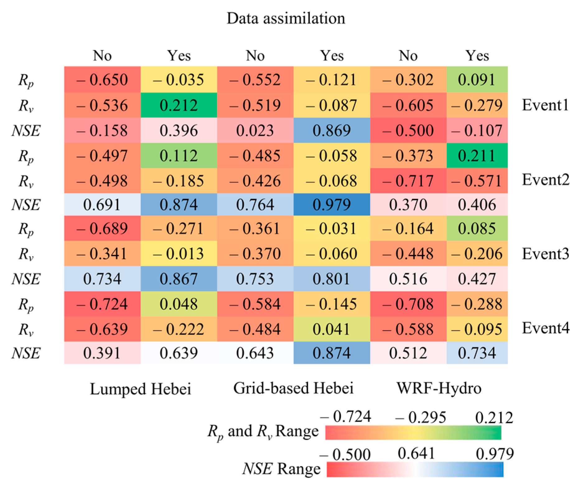
4.3. Effect of Data Assimilation on Coupled Systems with Variable Complexity

Smaller catchments are particularly vulnerable to uncertainties and spatial shifts in rainfall patterns that may result in poor streamflow performance [27]. Figure 10 illustrates the coupling systems’ stability from the grid-based model in blue, WRF-Hydro in yellow, and the lumped model in red. It can be observed that the CC for the grid-based model both before and after assimilation reached above 0.9 and that the values of RMSE were smaller than those of the other coupling systems, with the exception of Event 3. The lumped model had the next highest CC values, between 0.6 and 0.9, whereas WRF-Hydro exhibited a more scattered CC distribution. Nonetheless, after assimilation, the latter captured a better flood peak for Event 4. Detailed indices are given below for storm events, followed by further distinctions in between the effects of varying coupled systems under different types of rainfall before and after assimilation, as shown in Figure 11.

4.3.1. Results with the Lumped Hebei Model

Most lumped models lack the spatial information required to describe hydrological processes [56]. The lumped Hebei model consistently responds to spatial variability with probability functions (i.e., infiltration excess and saturation excess curves), thus ignoring the true spatial distribution. For the studied storms, the lumped model generally obtains an early flood peak for rainfall-runoff events, being 8 h and 4 h earlier for Event 3 and Event 4, respectively (Figure 6). Both Event 3 and Event 4 exhibited inhomogeneous spatial and temporal rainfall distributions. For the studied events, forecasts from the lumped model increased the inaccuracy of the peak present time. This may be due to the fact that when the catchment-averaged rainfall is used as an input, the effect of spatial variability in the underlying surface layer on runoff generation can only be considered when the spatial distribution of the rainfall is homogeneous (i.e., neither the combined effect of spatially heterogeneous rainfall distribution and underlying surface layer variability, nor the effect of net rainfall processes as multiple input sources when the spatial distribution of rainfall is heterogeneous).

4.3.2. Results with the Grid-Based Hebei Model

Based on the grid-based Hebei model, an atmospheric-hydrological coupling system was constructed for different rainfall resolutions and applied to the study area. This approach further demonstrated that descriptions of rainfall-runoff generation are compatible with local rainfall and flood forecasting, and that the grid-based Hebei model is more stable for forecasts both before and after assimilation compared with the other coupling systems tested. Flood forecasts before assimilation were slightly less accurate than WRF-Hydro for Event 1 and Event 2, but were generally better than the lumped model. Particularly, for the flood processes of Event 4, the grid-based Hebei model obtained the best NSE results (0.643 before assimilation and 0.874 after assimilation), demonstrating that this model is well-adapted to modeling flash floods. Although there was no clearly defined division of soil in the grid-based hydrological model, the influence of spatial heterogeneity due to soil type was somewhat reduced due to the relatively homogeneous nature of the study area.

4.3.3. Results with the WRF-Hydro Modeling System

WRF-Hydro exhibited the opposite prediction accuracy compared with the lumped model. A better forecast for the spatio-temporally heterogeneous Event 3 and Event 4 was noted than for Event 1. With the exception of Event 4, flooding processes were found to exhibit faster surface runoff recession, which may be related to rainfall-runoff generation and interactions between land surface that occurs at every short integration time step in the WRF-Hydro. This increased the volume of infiltrated precipitation, producing higher soil moisture and reducing runoff [57]. For Event 1, which had a small flood magnitude and long flood duration, the flood process was subject to a rapid recession, resulting in a poor NSE (−0.5 before assimilation and −0.107 after assimilation). Nevertheless, WRF-Hydro provided a more favorable forecast for Event 4, demonstrating its potential ability to predict flash floods. Overall, however, the accuracy of the WRF-Hydro forecasts was poor, supporting the findings of previous studies by Wang et al. [58] and Sharma et al. [31].

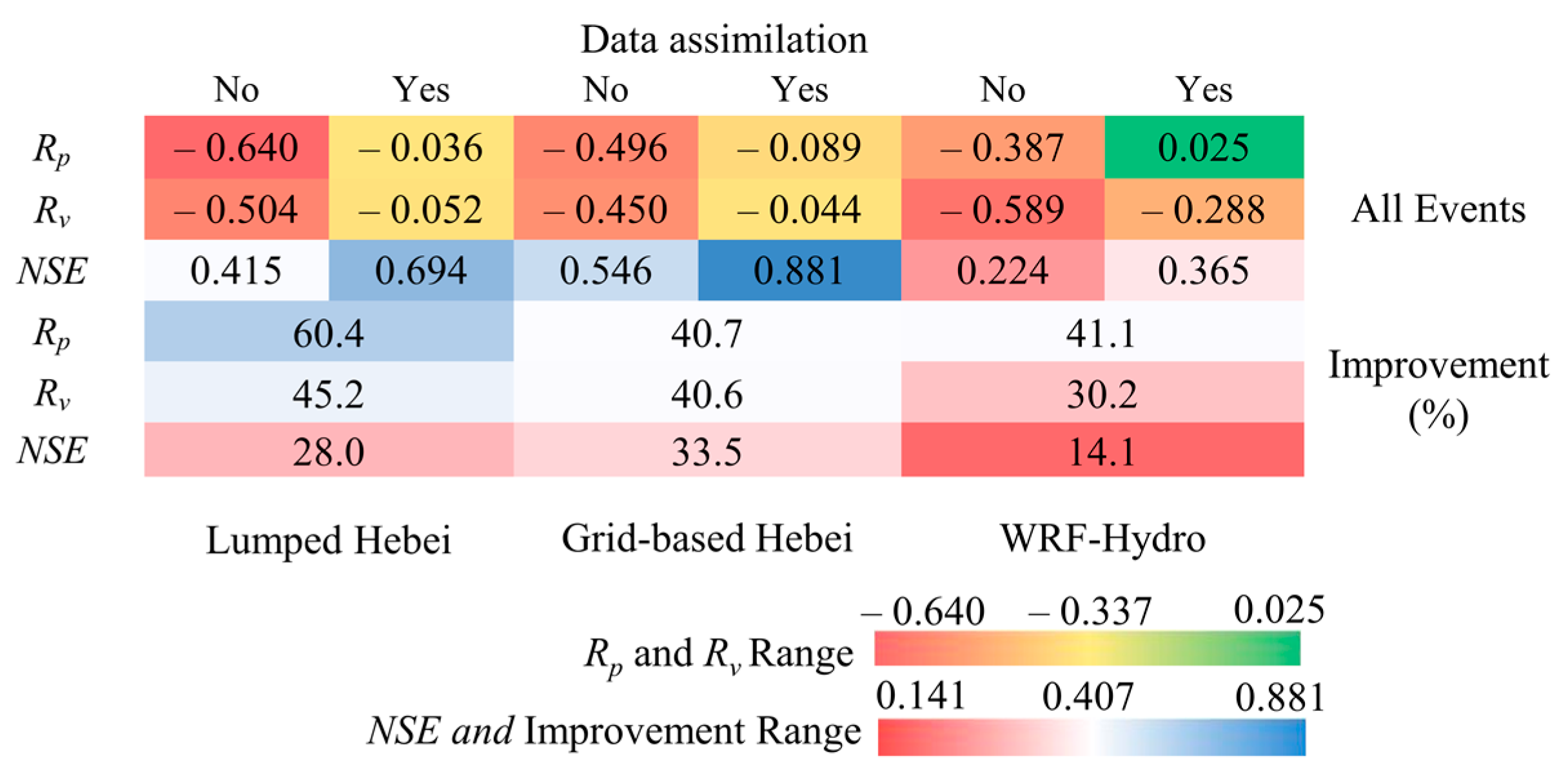
4.4. Improvement with Different Coupled Systems after Data Assimilation

Figure 12 provides further statistics on the extent to which the three coupled systems contribute to an overall improvement in response to flood events. The indices of systems were averaged from the results of the four studied storm events with different spatial and temporal characteristics.
Data assimilation promoted flooding in all three coupled systems. The coupling system using the lumped model had a weak response with no data assimilation, denoted by low Rp (−0.640) and Rv (−0.504) values, and therefore the most significant enhancement in Rp and Rv after assimilation, especially Rp, with an enhancement of 0.604. Before assimilation, the grid-based system was found to be more stable than the other two systems, so that the improvement was moderate among the three systems. For the WRF-Hydro system, responses to the Rp of Event 3 and Event 4, which were spatially and temporally heterogeneous rainfall events, was better before assimilation, but problems such as rapid surface runoff recession remain a concern. The improvements in Rp and Rv were more obvious after assimilation, whereas NSE was less improved.

5. Discussion

The forecasting accuracy of the flood peaks of the lumped model seems to be more demanding in terms of the accuracy of the input rainfall than the two other coupling systems, since the flood peaks of the lumped model were more moderate when unassimilated rainfall was poorly simulated such as in Event 4, where less than a quarter of the observed flood peaks were simulated before assimilation. Although the results of the corresponding indices were better following assimilation, this characteristic greatly increased the uncertainty of the atmospheric-hydrological coupling process, which can easily lead to errors when studying flash floods since it is difficult to guarantee the accuracy of the rainfall forecasting.
Although data assimilation improves the precipitation input required by WRF-Hydro, it is still insufficient for complex model systems due to the need to input more meteorological variables. To improve the performance of the coupled system in the prediction of hydrological processes, research on WRF-Hydro also includes the assimilation of soil moisture variables [59] and real-time flood assimilation. Indeed, the coupling system of the WRF-Hydro model has a stronger basis in physical processes than the former two coupled systems; however, the complexity of parameter estimation that emerges from the model also poses a greater challenge, which is a typical problem in many complex physics-based models such as the variable infiltration capacity model and the community land model (CLM) [60]. In addition to data assimilation, more precise expressions of regional rainfall-runoff mechanisms also need to be further explored. The hydrodynamic parameters developed for local areas may not necessarily be applicable to mesoscale areas; therefore, although the model structure is feasible, the parameters of WRF-Hydro in terms of soil properties are not fully calibrated for northern China. There is an urgent need to find easily available parameters and expression equations that reflect the spatial heterogeneity of local infiltration processes across the region as an alternative to model application.

6. Conclusions

In this study, WRF-3DVar data assimilation experiments were conducted, in which radar reflectivity and GTS data were assimilated with the involvement of coupled hydrological structures of different complexity for rainfall-runoff prediction. The performance of three atmospheric-hydrological systems, established by coupling WRF with the lumped Hebei model, the grid-based Hebei model, and the fully distributed WRF-Hydro, were compared and analyzed for storms with different temporal and spatial distribution characteristics before and after data assimilation. We further explored model potentials and limitations in the localization of flood events. Focusing on the impact of data assimilation on flood forecasting after improving different types of rainfall and coupling systems of varying complexity, we found that WRF-3DVar produces more accurate rainfall forecasts, and that the assimilated model system provides higher confidence in the flood forecasts.
When the lumped model was coupled, its input rainfall was averaged over all grid points at the catchment scale, which may conceal the potential advantages of high-resolution rainfall datasets. The grid-based Hebei model obtained better flood forecasting results, but it did not provide a more comprehensive description of the spatial and temporal processes of the land-surface hydrology. The WRF-Hydro system, on the other hand, is built on the basis of water balance and heat balance in terms of the physical processes, thus clearly necessary for future flood research. The main reasons for the lack of accuracy of the WRF-Hydro predictions might be the preciseness of the input meteorological elements and the structure of the modeling system. Demonstrating the former requires further exploration of the transition from multi-source data assimilation to multi-process data assimilation. The coupling system of WRF-Hydro may differ from actual regional characteristics in its representation of the rainfall-runoff mechanisms, and thus its spatial scale and applicability need to be further explored in the future, especially in relation to the high-resolution land surface and hydrological processes that are essential for flash flood forecasting. There is also a need for future work to build on the strengths of this model and tailor atmospheric-hydrological coupling systems to the study area.

Author Contributions

Conceptualization, W.W. and J.L.; Methodology, W.W., J.L., and F.Y.; Software, W.W. and Y.L.; Validation, W.W. and Y.L.; Formal analysis, W.W. and J.L.; Investigation, W.W., C.L., and F.Y.; Writing-original draft preparation, W.W. and J.L.; Writing-review and editing, W.W., J.L., and C.L.; Visualization, W.W.; Funding acquisition, J.L. and C.L. All authors have read and agreed to the published version of the manuscript.

Funding

This research was funded by the National Natural Science Foundation of China (51822906), the Major Science and Technology Program for Water Pollution Control and Treatment (2018ZX07110001), the National Key Research and Development Project (2017YFC1502405), and the IWHR Research & Development Support Program (WR0145B732017).

Conflicts of Interest

The authors declare no conflict of interest.

References

  1. Wang, W.; Seaman, N.L. A comparison study of convective parameterization schemes in a mesoscale model. Mon. Weather Rev. 1997, 125, 252–278. [Google Scholar] [CrossRef] [Green Version]
  2. Yousef, L.A.; Taha, B. Adaptation of water resources management to changing climate: The role of Intensity-Duration-Frequency curves. Int. J. Environ. Dev. 2015, 6, 478. [Google Scholar] [CrossRef] [Green Version]
  3. Yang, J.; Zhenming, J.I.; Chen, D.; Kang, S.; Congshen, F.U.; Duan, K.; Shen, M. Improved Land Use and Leaf Area Index Enhances WRF-3DVAR Satellite Radiance Assimilation: A Case Study Focusing on Rainfall Simulation in the Shule River Basin during July 2013. Adv. Atmos. Sci. 2018, 35, 628–644. [Google Scholar] [CrossRef]
  4. Yucel, I.; Onen, A.; Yilmaz, K.K.; Gochis, D.J. Calibration and evaluation of a flood forecasting system: Utility of numerical weather prediction model, data assimilation and satellite-based rainfall. J. Hydrol. 2015, 523, 49–66. [Google Scholar] [CrossRef] [Green Version]
  5. Bao, H.; Li, Z.; Yu, Z. Development of coupled atmospheric-hydrologic-hydraulic flood forecasting system driven by ensemble weather predictions. AGUFM 2009, 2009, H51G-0833. [Google Scholar] [CrossRef]
  6. Ferretti, R.; Lombardi, A.; Tomassetti, B.; Sangelantoni, L.; Colaiuda, V.; Mazzarella, V.; Maiello, I.; Verdecchia, M.; Redaelli, G. Regional ensemble forecast for early warning system over small Apennine catchments on Central Italy. Hydrol. Earth Syst. Sci. Discuss. 2019, 1–25. [Google Scholar] [CrossRef]
  7. Sokol, Z. Assimilation of extrapolated radar reflectivity into a NWP model and its impact on a precipitation forecast at high resolution. Atmos. Res. 2011, 100, 201–212. [Google Scholar] [CrossRef]
  8. Mohanty, U.C.; Routray, A.; Osuri, K.K.; Prasad, S.K. A Study on Simulation of Heavy Rainfall Events over Indian Region with ARW-3DVAR Modeling System. Pure Appl. Geophys. 2012, 169, 381–399. [Google Scholar] [CrossRef]
  9. Routray, A.; Mohanty, U.; Niyogi, D.; Rizvi, S.; Osuri, K.K. Simulation of heavy rainfall events over Indian monsoon region using WRF-3DVAR data assimilation system. Meteorol. Atmos. Phys. 2010, 106, 107–125. [Google Scholar] [CrossRef]
  10. Kumar, P.; Varma, A.K. Assimilation of INSAT-3D hydro-estimator method retrieved rainfall for short-range weather prediction. Q. J. R. Meteorolog. Soc. 2016, 143, 384–394. [Google Scholar] [CrossRef]
  11. Fierro, A.O.; Clark, A.J.; Mansell, E.R.; MacGorman, D.R.; Dembek, S.R.; Ziegler, C.L. Impact of storm-scale lightning data assimilation on WRF-ARW precipitation forecasts during the 2013 warm season over the contiguous United States. Mon. Weather Rev. 2015, 143, 757–777. [Google Scholar] [CrossRef]
  12. Yesubabu, V.; Srinivas, C.V.; Langodan, S.; Hoteit, I. Predicting extreme rainfall events over Jeddah, Saudi Arabia: Impact of data assimilation with conventional and satellite observations. Q. J. R. Meteorolog. Soc. 2016, 142, 327–348. [Google Scholar] [CrossRef] [Green Version]
  13. Lin, C.A.; Wen, L.; Lu, G.; Wu, Z.; Zhang, J.; Yang, Y.; Zhu, Y.; Tong, L. Atmospheric-hydrological modeling of severe precipitation and floods in the Huaihe River Basin, China. J. Hydrol. 2006, 330, 249–259. [Google Scholar] [CrossRef]
  14. Lu, G.; Wu, Z.; Wen, L.; Lin, C.A.; Zhang, J.; Yang, Y. Real-time flood forecast and flood alert map over the Huaihe River Basin in China using a coupled hydro-meteorological modeling system. Sci. China Ser. E Technol. Sci. 2008, 51, 1049–1063. [Google Scholar] [CrossRef]
  15. Lin, C.A.; Wen, L.; Lu, G.; Wu, Z.; Zhang, J.; Yang, Y.; Zhu, Y.; Tong, L. Real-time forecast of the 2005 and 2007 summer severe floods in the Huaihe River Basin of China. J. Hydrol. 2010, 381, 33–41. [Google Scholar] [CrossRef]
  16. Wu, J.; Lu, G.; Wu, Z. Flood forecasts based on multi-model ensemble precipitation forecasting using a coupled atmospheric-hydrological modeling system. Nat. Hazards 2014. [Google Scholar] [CrossRef]
  17. Moser, B.A.; Gallus, W.A., Jr.; Mantilla, R. An initial assessment of radar data assimilation on warm season rainfall forecasts for use in hydrologic models. Weather Forecast 2015, 30, 1491–1520. [Google Scholar] [CrossRef]
  18. Yang, D.; Herath, S.; Musiake, K. Comparison of different distributed hydrological models for characterization of catchment spatial variability. Hydrol. Process. 2000, 14, 403–416. [Google Scholar] [CrossRef]
  19. Essou, G.R.C.; Arsenault, R.; Brissette, F. Comparison of climate datasets for lumped hydrological modeling over the continental United States. J. Hydrol. 2016, 537, 334–345. [Google Scholar] [CrossRef]
  20. Solomatine, D.P.; Dulal, K.N. Model trees as an alternative to neural networks in rainfall—runoff modelling. Hydrol. Sci. J. 2003, 48, 399–411. [Google Scholar] [CrossRef]
  21. Bray, M.; Han, D. Identification of support vector machines for runoff modelling. J. Hydroinf. 2004, 6, 265–280. [Google Scholar] [CrossRef] [Green Version]
  22. Karpatne, A.; Atluri, G.; Faghmous, J.H.; Steinbach, M.; Banerjee, A.; Ganguly, A.; Shekhar, S.; Samatova, N.; Kumar, V. Theory-guided data science: A new paradigm for scientific discovery from data. IEEE Trans. Knowl. Data Eng. 2017, 29, 2318–2331. [Google Scholar] [CrossRef]
  23. Herath, H.M.V.V.; Chadalawada, J.; Babovic, V. Hydrologically Informed Machine Learning for Rainfall-Runoff Modelling: Towards Distributed Modelling. Hydrol. Earth Syst. Sci. Discuss. 2020, 487, 1–42. [Google Scholar] [CrossRef]
  24. Cho, Y.; Engel, B.A. NEXRAD Quantitative Precipitation Estimations for Hydrologic Simulation Using a Hybrid Hydrologic Model. J. Hydrometeorol. 2017, 18, 25–47. [Google Scholar] [CrossRef]
  25. Song, X.; Zhang, J.; Zhan, C.; Xuan, Y.; Ye, M.; Xu, C. Global sensitivity analysis in hydrological modeling: Review of concepts, methods, theoretical framework, and applications. J. Hydrol. 2015, 523, 739–757. [Google Scholar] [CrossRef] [Green Version]
  26. Fatichi, S.; Vivoni, E.R.; Ogden, F.L.; Ivanov, V.Y.; Mirus, B.B.; Gochis, D.J.; Downer, C.W.; Camporese, M.; Davison, J.H.; Ebel, B.A. An overview of current applications, challenges, and future trends in distributed process-based models in hydrology. J. Hydrol. 2016, 537, 45–60. [Google Scholar] [CrossRef] [Green Version]
  27. Wagner, S.; Fersch, B.; Yuan, F.; Yu, Z.; Kunstmann, H. Fully coupled atmospheric-hydrological modeling at regional and long-term scales: Development, application, and analysis of WRF-HMS. Water Resour. Res. 2016. [Google Scholar] [CrossRef] [Green Version]
  28. Liu, J.; Wang, J.; Pan, S.; Tang, K.; Li, C.; Han, D. A real-time flood forecasting system with dual updating of the NWP rainfall and the river flow. Nat. Hazards 2015, 77, 1161–1182. [Google Scholar] [CrossRef]
  29. Li, J.; Chen, Y.; Wang, H.; Qin, J.; Li, J.; Chiao, S. Extending flood forecasting lead time in a large watershed by coupling WRF QPF with a distributed hydrological model. Hydrol. Earth Syst. Sci. 2017, 21, 1279. [Google Scholar] [CrossRef] [Green Version]
  30. Rogelis, M.C. Streamflow forecasts from WRF precipitation for flood early warning in mountain tropical areas. Hydrol. Earth Syst. Sci. 2018, 22, 853–870. [Google Scholar] [CrossRef] [Green Version]
  31. Sharma, S.; Siddique, R.; Reed, S.; Ahnert, P.; Mejia, A. Hydrological Model Diversity Enhances Streamflow Forecast Skill at Short- to Medium-Range Timescales. Water Resour. Res. 2019, 55, 1510–1530. [Google Scholar] [CrossRef]
  32. Haddeland, I.; Clark, D.B.; Franssen, W.; Ludwig, F.; Voß, F.; Arnell, N.W.; Bertrand, N.; Best, M.; Folwell, S.; Gerten, D. Multimodel estimate of the global terrestrial water balance: Setup and first results. J. Hydrometeorol. 2011, 12, 869–884. [Google Scholar] [CrossRef] [Green Version]
  33. Wood, E.F.; Roundy, J.K.; Troy, T.J.; Van Beek, L.; Bierkens, M.F.; Blyth, E.; de Roo, A.; Döll, P.; Ek, M.; Famiglietti, J. Hyperresolution global land surface modeling: Meeting a grand challenge for monitoring Earth’s terrestrial water. Water Resour. Res. 2011, 47. [Google Scholar] [CrossRef]
  34. Wang, W.; Liu, J.; Li, C.; Liu, Y.; Yu, F.; Yu, E. An Evaluation Study of the Fully Coupled WRF/WRF-Hydro Modeling System for Simulation of Storm Events with Different Rainfall Evenness in Space and Time. Water 2020, 12, 1209. [Google Scholar] [CrossRef]
  35. Fiori, E.; Comellas, A.; Molini, L.; Rebora, N.; Siccardi, F.; Gochis, D.; Tanelli, S.; Parodi, A. Analysis and hindcast simulations of an extreme rainfall event in the Mediterranean area: The Genoa 2011 case. Atmos. Res. 2014, 138, 13–29. [Google Scholar] [CrossRef] [Green Version]
  36. Verri, G.; Pinardi, N.; Gochis, D.; Tribbia, J.; Navarra, A.; Coppini, G.; Vukicevic, T. A meteo-hydrological modelling system for the reconstruction of river runoff: The case of the Ofanto river catchment. Nat. Hazards Earth Syst. Sci. 2017, 17, 1741–1761. [Google Scholar] [CrossRef] [Green Version]
  37. Moeng, C.H.; Dudhia, J.; Klemp, J.; Sullivan, P. Examining Two-Way Grid Nesting for Large Eddy Simulation of the PBL Using the WRF Model. Mon. Weather Rev. 2007, 135, 2295–2311. [Google Scholar] [CrossRef]
  38. Shin, H.H.; Hong, S.-Y. Analysis of resolved and parameterized vertical transports in convective boundary layers at gray-zone resolutions. J. Atmos. Sci. 2013, 70, 3248–3261. [Google Scholar] [CrossRef]
  39. Tian, J.; Liu, J.; Yan, D.; Li, C.; Yu, F. Numerical rainfall simulation with different spatial and temporal evenness by using a WRF multiphysics ensemble. Nat. Hazards Earth Syst. Sci. 2017, 17, 563–579. [Google Scholar] [CrossRef] [Green Version]
  40. Tian, J.; Liu, J.; Wang, J.; Li, C.; Yu, F.; Chu, Z. A spatio-temporal evaluation of the WRF physical parameterisations for numerical rainfall simulation in semi-humid and semi-arid catchments of Northern China. Atmos. Res. 2017, 191, 141–155. [Google Scholar] [CrossRef]
  41. Lin, Y.-L.; Farley, R.D.; Orville, H.D. Bulk parameterization of the snow field in a cloud model. J. Clim. Appl. Meteorol. 1983, 22, 1065–1092. [Google Scholar] [CrossRef] [Green Version]
  42. Hong, S.Y.; Noh, Y.; Dudhia, J. A new vertical diffusion package with an explicit treatment of entrainment processes. Mon. Weather Rev. 2006, 134, 2318–2341. [Google Scholar] [CrossRef] [Green Version]
  43. Kain, J.S. The Kain–Fritsch convective parameterization: An update. J. Appl. Meteorol. 2004, 43, 170–181. [Google Scholar] [CrossRef] [Green Version]
  44. Grell, G.A.; Freitas, S.R. A scale and aerosol aware stochastic convective parameterization for weather and air quality modeling. Atmos. Chem. Phys. 2014, 13, 5233–5250. [Google Scholar] [CrossRef] [Green Version]
  45. Janjić, Z.I. The Step-Mountain Eta Coordinate Model: Further Developments of the Convection, Viscous Sublayer, and Turbulence Closure Schemes. Mon. Weather Rev. 1994, 122, 927–945. [Google Scholar] [CrossRef] [Green Version]
  46. Tian, J.; Liu, J.; Yan, D.; Li, C.; Chu, Z.; Yu, F. An assimilation test of Doppler radar reflectivity and radial velocity from different height layers in improving the WRF rainfall forecasts. Atmos. Res. 2017, 198, 132–144. [Google Scholar] [CrossRef]
  47. Liu, J.; Tian, J.; Yan, D.; Li, C.; Yu, F.; Shen, F. Evaluation of Doppler radar and GTS data assimilation for NWP rainfall prediction of an extreme summer storm in northern China: From the hydrological perspective. Hydrol. Earth Syst. Sci. 2018, 22, 4329–4348. [Google Scholar] [CrossRef] [Green Version]
  48. Beven, K.J. Physically based, variable contibution area model of basin hydrology. Hydrol. Ences. Bull. 1979, 24. [Google Scholar] [CrossRef] [Green Version]
  49. Beven, K. Surface water hydrology-runoff generation and basin structure. Rev. Geophys. 1983, 21, 721–730. [Google Scholar] [CrossRef]
  50. Tian, J.; Liu, J.; Wang, Y.; Wang, W.; Li, C.; Hu, C. A coupled atmospheric-hydrologic modeling system with variable grid sizes for rainfall-runoff simulation in semi-humid and semi-arid watersheds: How does the coupling scale affects the results? Hydrol. Earth Syst. Sci. 2020, 24, 3933–3949. [Google Scholar] [CrossRef]
  51. Gochis, D.J.; Chen, F. Hydrological Enhancements to the Community Noah Land Surface Model: Technical Description; NCAR Tech. Note, TN-454+STR, Boulder, Colo.; University Corporation for Atmospheric Research: Boulder, CO, USA, 2003; 77p. [Google Scholar] [CrossRef]
  52. Schaake, J.C.; Koren, V.I.; Duan, Q.-Y.; Mitchell, K.; Chen, F. Simple water balance model for estimating runoff at different spatial and temporal scales. J. Geophys. Res. Atmos. 1996, 101, 7461–7475. [Google Scholar] [CrossRef]
  53. Wigmosta, M.S.; Lettenmaier, D.P. A comparison of simplified methods for routing topographically driven subsurface flow. Water Resour. Res. 1999, 35, 255–264. [Google Scholar] [CrossRef]
  54. Downer, C.W.; Ogden, F.L.; Martin, W.D.; Harmon, R.S. Theory, development, and applicability of the surface water hydrologic model CASC2D. Hydrol. Process. 2002, 16, 255–275. [Google Scholar] [CrossRef]
  55. Gochis, D.; Barlage, M.; Dugger, A.; FitzGerald, K.; Karsten, L.; McAllister, M.; McCreight, J.; Mills, J.; RefieeiNasab, A.; Read, L. The WRF-Hydro modeling system technical description (Version 5.0). NCAR Tech. Note 2018, 107. [Google Scholar] [CrossRef]
  56. Moore, R. The probability-distributed principle and runoff production at point and basin scales. Hydrol. Sci. J. 1985, 30, 273–297. [Google Scholar] [CrossRef] [Green Version]
  57. Cuntz, M.; Mai, J.; Samaniego, L.; Clark, M.; Wulfmeyer, V.; Branch, O.; Attinger, S.; Thober, S. The impact of standard and hard-coded parameters on the hydrologic fluxes in the Noah-MP land surface model. J. Geophys. Res. Atmos. 2016, 121, 10676–10700. [Google Scholar] [CrossRef]
  58. Wang, Y.; Lahmers, T.; Hazenberg, P.; Gupta, H.; Castro, C.; Gochis, D.; Dugger, A.; Yates, D.; Read, L.; Karsten, L. Enhancements to the WRF-Hydro Hydrologic Model Structure for Semi-arid Environments. AGUFM 2018, 2018, H41P-2347. [Google Scholar]
  59. Zarekarizi, M. Ensemble Data Assimilation for Flood Forecasting in Operational Settings: From Noah-MP to WRF-Hydro and the National Water Model. J. Hydrol. 2018. [Google Scholar] [CrossRef]
  60. Xi, C.; Yang, T.; Wang, X.; Xu, C.Y.; Yu, Z. Uncertainty Intercomparison of Different Hydrological Models in Simulating Extreme Flows. Water Resour. Manag. 2012, 27, 1393–1409. [Google Scholar] [CrossRef]
Figure 1. Locations of the Fuping and Zijingguan catchments covered by the weather research forecasting (WRF) nested domains and the weather radar.
Remotesensing 13 00595 g001
Figure 2. Observed rainfall-runoff processes for the four selected storm events.
Remotesensing 13 00595 g002
Figure 3. The cycling data assimilation process for Event 4.
Remotesensing 13 00595 g003
Figure 4. Rainfall-runoff mechanisms for the grid-based Hebei model.
Remotesensing 13 00595 g004
Figure 5. Framework for the coupled atmospheric-hydrologic modeling systems used for rainfall-runoff prediction.
Remotesensing 13 00595 g005
Figure 6. Rainfall-runoff predictions for the three atmospheric-hydrologic coupled systems before and after data assimilation: (a) Lumped Hebei; (b) Grid-based Hebei; (c) WRF-Hydro.
Remotesensing 13 00595 g006
Figure 7. Cumulative rainfall curves before and after data assimilation under different assimilation run conditions.
Remotesensing 13 00595 g007
Figure 8. Taylor diagrams of forecasted hourly cumulative rainfall before and after data assimilation.
Remotesensing 13 00595 g008
Figure 9. Averaged runoff prediction indices for NSE, Rv, and Rp of the four storm events.
Remotesensing 13 00595 g009
Figure 10. Taylor diagrams of forecasted hourly runoff before and after data assimilation.
Remotesensing 13 00595 g010
Figure 11. Runoff prediction indices of NSE, Rv, and Rp for different atmospheric-hydrologic modeling systems.
Remotesensing 13 00595 g011
Figure 12. Improvement of the forecasted runoff indices of NSE, Rv, and Rp for the three coupled systems.
Remotesensing 13 00595 g012
Table 1. Storm events and spatio-temporal rainfall evenness characterized by Cv.
Storm
Event
CatchmentStorm Duration24 h Rainfall Accumulation (mm)Peak Flow (m3/s)Temporal CvSpatial Cv
Even 1Fuping29 July 2007 20:00 to 30 July 2007 20:0063.429.70.60110.3975
Event 2Fuping30 July 2012 10:00 to 31 July 2012 10:0050.570.71.08230.1927
Event 3Fuping11 August 2013 07:00 to 12 August 2013 07:0030.946.62.39250.7400
Event 4Zijingguan21 July 2012 04:00 to 22 July 2012 04:00172.22580.01.88650.6098
Table 2. Detailed configurations of the weather research forecasting (WRF).
SubjectChosen OptionSubjectChosen Option
Driving dataGFS each 6 hWRF output interval1 h
Integration time stepDom1: 18 sdomain center39°04′15″ N, 113°59′26″ E
Dom2: 6 sVertical discretization40 layers
Horizontal resolutionDom1: 9 kmPressure50 hPa
Dom2: 3 kmProjection resolutionLambert
Horizontal grid numberDom1: 140 × 140Longwave radiationRRTM
Dom2: 150 × 120Shortwave radiationDudhia
Table 3. Optimal physical parameterization for the studied storm events.
Ensemble ScenariosEvent 1Event 2Event 3Event 4
Microphysics schemeLin
WSM6
Cumulus convectionKF
GD
Planetary boundary layerYSU
MYJ
Table 4. Observed and forecasted rainfall accumulation before and after data assimilation.
Storm EventObservedNo Data AssimilationData AssimilationImprovement
ForecastedREForecastedREForecastedRE
Event 163.3849.35−0.22167.460.06418.110.157
Event 250.4837.22−0.26352.180.03414.960.229
Event 330.8219.05−0.38229.58−0.04010.530.342
Event 4172.17128.36−0.254148.12−0.14019.760.114
Average79.2158.49−0.28074.34−0.02015.850.260
Publisher’s Note: MDPI stays neutral with regard to jurisdictional claims in published maps and institutional affiliations.

