A First Approach to Aerosol Classification Using Space-Borne Measurement Data: Machine Learning-Based Algorithm and Evaluation

Abstract

A new method was developed for classifying aerosol types involving a machine-learning approach to the use of satellite data. An Aerosol Robotic NETwork (AERONET)-based aerosol-type dataset was used as a target variable in a random forest (RF) model. The contributions of satellite input variables to the RF-based model were quantified to determine an optimal set of input variables. The new method, based on inputs of satellite variables, allows the classification of seven aerosol types: pure dust, dust-dominant mixed, pollution-dominant mixed aerosols, and pollution aerosols (strongly, moderately, weakly, and non-absorbing). The performance of the model was statistically evaluated using AERONET data excluded from the model training dataset. Model accuracy for classifying the seven aerosol types was 59%, improving to 72% for four types (pure dust, dust-dominant mixed, strongly absorbing, and non-absorbing). The performance of the model was evaluated against an earlier aerosol classification method based on the wavelength dependence of single-scattering albedo (SSA) and fine-mode-fraction values from AERONET. Typical wavelength dependences of SSA for individual aerosol types are consistent with those obtained for aerosol types by the new method. This study demonstrates that an RF-based model is capable of satellite aerosol classification with sensitivity to the contribution of non-spherical particles.

1. Introduction

Atmospheric aerosols are known to have both direct and indirect effects on Earth’s climate since aerosols scatter and absorb solar radiation and affect cloud microphysical properties [1]. The diverse and significant effects of aerosols on climate play a critical role in radiative forcing, which has high uncertainty [2]. To estimate aerosol radiative forcing, aerosol type has been identified as the important parameters because aerosol properties, such as radiation absorptivity and particle size, differ among aerosol types [3,4]. In addition, the aerosol type is an input parameter of satellite aerosol retrieval algorithms and affects their accuracy [5,6]. Therefore, accurate aerosol classification is essential for valid climate and satellite aerosol remote sensing.

Several satellite aerosol-type classification algorithms have been developed based on the threshold approach. Higurashi and Nakajima [3] developed a four-channel algorithm (4CA) to detect aerosol types using four-channel data from Sea-viewing Wide Field of View Sensors (SeaWiFS). Four aerosol types, including soil dust, carbonaceous, sulfate, and sea salt, have been detected over the ocean in northeastern Asia [3]. Jeong and Li [7] proposed an aerosol classification method using Advanced Very High Resolution Radiometer (AVHRR) and Total Ozone Mapping Spectrometer (TOMS) data. Aerosol optical thickness (AOT) and Ångström exponent (AE) from AVHRR and the aerosol index from TOMS were used to classify aerosols into seven types (biomass burning, dust, sea salt, pollution/sulfate mixtures, biomass/dust mixtures, sulfate/sea salt mixtures, and undefined mixtures) on a global scale. Lee et al. [8] classified aerosols into four major types (dust, sea salt, smoke, and sulfate) and two mixtures of major types using AOT and AE from Moderate Resolution Imaging Spectroradiometer (MODIS) data and aerosol index from Ozone Monitoring Instrument (OMI) data over northeastern Asia. Those authors also investigated the spatial and frequency distribution of aerosol types over northeastern Asia and made a comparison with those obtained from a global aerosol climate model [8]. Kim et al. [9] suggested a MODIS–OMI algorithm (MOA) with aerosol index from OMI and Fine Mode Fraction (FMF) from MODIS to classify aerosol types. The classification results of the MOA were compared with 4CA over northeastern Asia, and their agreement ranged from 32% to 81% [9]. In addition to channel data and aerosol optical properties, Torres et al. [6] introduced the use of carbon monoxide (CO), a tracer of carbonaceous aerosols, to distinguish between carbonaceous and dust aerosols instead of AE. Column amounts of CO from the Atmospheric Infrared Sounder (AIRS) and aerosol index were used to classify aerosol types in an operational OMI near-UV aerosol algorithm [6]. Penning de Vries et al. [10] developed a new global aerosol classification algorithm (GACA) using monthly mean aerosol properties (aerosol optical depth (AOD) and AE) and column densities of trace gases (NO₂, HCHO, SO₂, and CO). The GACA classified aerosol types on a monthly basis, and the results were compared against model-derived aerosol compositions from the global monitoring atmospheric composition and climate model. Mao et al. [11] utilized AOD and aerosol relative optical depth from MODIS to classify aerosol types over eight study regions including major aerosol source regions and downwind of the source regions. The agreement between the satellite-based results and ground-based results ranges from 36% to 91% over the study regions in Mao et al. [11]. In fact, Mao et al. [11] is the only one of the aforementioned satellite aerosol classification studies that attempted such a satellite and ground-based validation. Most of the classification results have been compared only with results from an aerosol climate model and earlier aerosol classification methods. Although the accuracy assessments of aerosol classification methods have rarely been carried out, uncertainties in satellite aerosol optical properties and trace gas products have been reported. The uncertainty of MODIS-derived AOD was found to be ±(0.05 + 0.15 × AOD) according to Chu et al. [12], and that of MODIS AE was up to 30% [13]. The uncertainty in AIRS CO products is 15% as reported in Thrastarson et al. [14]. These uncertainties associated with satellite input variables can lead to misclassifications of aerosol types in threshold-based classification methods.

Aerosol type classification methods have also been developed using Aerosol Robotic NETwork (AERONET) data, which are used to evaluate satellite aerosol products. Previous studies have established an AERONET-based aerosol classification method using several aerosol optical properties, including single scattering albedo (SSA), FMF, AOD, and AE obtained from an AERONET version 2 inversion product [15,16,17]. Recently, the AERONET version 3 inversion product was released, which provides particle depolarization ratios at 440, 675, 870, and 1020 nm and thus is sensitive to aerosol particle shape [18,19]. The AERONET-derived depolarization ratio values at several wavelengths were found to be highly correlated compared with those obtained from ground-based light detection and ranging (lidar) measurements [20]. Zo and Shin [19] reported a potential for depolarization ratio values for identifying the contribution of aerosol types in aerosol particle mixtures. Shin et al. [21] suggested a new aerosol type classification method using SSA to distinguish the aerosol absorbance and dust ratio (R_d) derived from particle linear depolarization ratios (PLDR), which consider contributions of non-spherical particles, such as dust aerosols, from AERONET version 3 inversion products. It was reported that R_d is a more suitable parameter for identifying aerosol types mixed with dust particles than FMF, as non-spherical dust aerosols might be present in the fine mode [21]. The aerosol classification method suggested by Shin et al. [21] identified aerosol types mixed with spherical and non-spherical particles in East Asia as well as other global sites, indicating a possibility as an evaluation tool of the satellite aerosol type classification methods. However, PLDR is not available in satellite measurements except for Aerosol Lidar with Orthogonal Polarization (CALIOP), which has 16 days of global coverage. Therefore, it is necessary to investigate new satellite-based parameters that can identify the contribution of non-spherical particles without PLDR.

Recently, machine learning techniques have been applied to satellite remote sensing of aerosol information that is difficult to fully estimate via traditional regression models and physical retrieval approaches. In particular, various machine learning models have been introduced to estimate surface concentrations of particulate matter (PM) using satellite measurements and meteorological data [22,23,24,25,26,27]. In addition to estimates of ground-level PM concentrations, machine-learning techniques have been used to estimate AOD and aerosol height (the altitude of peak aerosol concentration in a vertical profile). Han and Sohn [28] retrieved AOT and dust height using a statistical artificial neural network (NN) approach. The artificial NN-based model was trained by relating brightness temperature, surface elevation, and relative air mass from AIRS measurements to MODIS-derived AOT and dust height from CALIOP data. Chimot et al. [29] developed an aerosol layer height retrieval algorithm based on a multilayer perceptron NN model using an absorption band of an O₂–O₂ collision pair measured by OMI. Therefore, machine-learning-based techniques have been increasingly and successfully applied to solving challenging problems in aerosol remote sensing. Inspired by this, we attempted to apply the method to satellite-based aerosol type classification using data classified according to an AERONET-based method [21]. Such a trained aerosol classification model may be able to identify contributions of non-spherical particles using only satellite-based variables without the input of AERONET observations.

Accordingly, we propose a new machine-learning method for classifying aerosol types based on satellite observations. Various satellite input variables associated with aerosol properties and their production were introduced. Several aerosol optical properties were obtained from MODIS measurements, which have been used in various aerosol classification methods in previous studies. Aerosol index and trace gas information were obtained from TROPOspheric Monitoring Instrument (TROPOMI) measurements, which is a recent environmental sensor similar to OMI but with improved spatial resolution. Among the various satellite input parameters, we aimed to adopt an optimal input variable set such that missing data were minimized and classification accuracy maximized. Therefore, we adopted a random forest (RF) model, which provides a measure of importance for each input variable. The RF-based model was trained with input variables consisting of satellite data and a target variable of the AERONET-based aerosol type dataset. The performance of the RF-based model was statistically evaluated using an AERONET-based aerosol type dataset, which was excluded from the model training dataset. For the first time, the results were also evaluated using wavelength dependence of SSA and FMF values from AERONET measurements. In addition, the performance of earlier threshold-based aerosol classification methods was investigated via comparison with the AERONET-based aerosol type dataset.

2. Variables and Data Collection

We classified aerosol types using satellite measurements based on an RF approach (Figure 1). The RF model was trained with a set of observational data consisting of a target variable (i.e., aerosol types) and input variables (i.e., satellite measurements). The target variable dataset was constructed from the AERONET-based classification method suggested by Shin et al. [21]. For the satellite input variables, we selected input variable candidates prior to the determination of the optimal input variable set; this minimized missing data and maximized classification accuracy. Various satellite input variable candidates were selected, including new variables related to aerosol properties and their production as well as previously used satellite input variables.

2.1. Target Variable Dataset

The target variable (aerosol-type) dataset was constructed using an AERONET-based aerosol classification method [21]. Shin et al. [21] suggested a method utilizing PLDR and SSA data at 1020 nm from the AERONET version 3 inversion product. In the work of Shin et al. [21], the R_d was introduced to identify spherical and non-spherical particles (i.e., dust aerosols). The R_d can be defined using the PLDR [30,31]. Shin et al. [21] utilized the PLDR at 1020 nm to calculate the R_d, as AERONET-derived PLDR data at 1020 nm were reported to have the highest correlation with lidar PLDR [20]. The R_d is expressed as:

$$R_d=\frac{\left(\delta -{\delta }_{nd}\right)\left(1+{\delta }_d\right)}{\left({\delta }_d-{\delta }_{nd}\right)\left(1+\delta \right)}$$

(1)

where ${\delta }_{nd}$ and ${\delta }_d$ indicate the PLDR (δ) of non-dust and pure dust particles, respectively. The values used for ${\delta }_{nd}$ and ${\delta }_d$ were 0.02 and 0.30, respectively, as suggested by Shin et al. [21]. The R_d is set to 0 when PLDR is lower than ${\delta }_{nd}$, which indicates spherical (e.g., anthropogenic or smoke) particles [21]. In contrast, the R_d is set to 1 when PLDR is higher than 0.30, which shows a higher contribution of dust aerosols.

In the AERONET-based aerosol classification algorithm [21], R_d is utilized to identify the contribution of dust aerosols. Pure dust (PD), dust dominated mixture (DDM), and pollution dominated mixture (PDM) are classified according to R_d thresholds:

(1)

PD: 0.89 < R_d

(2)

DDM: 0.53 ≤ R_d ≤ 0.89

(3)

PDM: 0.17 ≤ R_d < 0.53

When R_d is less than 0.17, an aerosol is classified as a pollution particle. The SSA at 1020 nm is used to distinguish the absorption characteristics of pollution particles:

(1)

Non-absorbing (NA): 0.95 < SSA

(2)

Weakly absorbing (WA): 0.90 < SSA ≤ 0.95

(3)

Moderately absorbing (MA): 0.85 ≤ SSA ≤ 0.90

(4)

Strongly absorbing (SA): SSA < 0.85

The NA type represents non-absorbing fine-mode aerosols (e.g., sulfate and nitrate). Thus, the SA type indicates strongly absorbing fine-mode aerosols, such as carbonaceous aerosols.

The target variable dataset was constructed using AERONET measurements from January 2018 to July 2020, as TROPOMI data are available from 2018. Both AERONET Level 1.5 (cloud-screened) and Level 2.0 (quality-assured) data were collected at the overpass time (13:30 local time (LT)) of TROPOMI aboard the Sentinel-5P satellite and MODIS aboard the Aqua satellite. To minimize uncertainties in AERONET Level 1.5 data, we collected data only when AOD at 440 nm was above 0.4; i.e., the SSA data processing criterion of AERONET Level 2.0. For AERONET Level 1.5 and 2.0 data, a total of 10,481 or 2232 data points were collected over 300 or 161 sites, respectively. A map of AERONET stations that provided PLDR and SSA data during the study period for Level 1.5 and 2.0 data is shown in Figure 2.

Although AERONET Level 2.0 assures the quality of the data, the dataset includes only 2232 cases, with seven classes (aerosol types) being too small to train a machine-learning system. There were only 108 PD cases in the dataset. For AERONET Level 1.5 data, the sites were more globally distributed than those from which Level 2.0 data were collected (Figure 2). Therefore, we used mainly the AERONET Level 1.5 dataset (AOD > 0.4) to provide more training cases than are available from the AERONET Level 2.0 dataset, together with partial use of the AERONET Level 2.0 dataset (in Section 4 only).

2.2. Satellite Input Variable Candidates

The input variable candidates were first selected based on previous aerosol classification methods. Among FMF and AE (a measure of aerosol size), AE was selected, as used in previous studies [7,8], while FMF was excluded due to more missing values than AE. AOD was used to identify the presence of aerosols in previous satellite classification algorithms [7,8,9]. Therefore, we also selected AOD as one of the candidates for input variables. The aerosol index was selected as one of the candidates for input variables to account for the presence of absorbing aerosols, as it has been used in several satellite aerosol classification methods [6,7,8,9]. However, SSA values have been excluded due to many missing values in the MODIS aerosol product. In addition to the parameters directly related to aerosol optical properties, Torres et al. [6] introduced column CO amount to identify the presence of carbonaceous particles that we also adopted. Penning de Vries et al. [10] also utilized trace gas abundances (NO₂, SO₂, HCHO, and CO) for monthly aerosol-type classification, since AOD is reported to be significantly correlated with trace gas concentrations [32]. These trace gas column densities were used to infer the dominating source of the aerosols in Penning de Vries et al. [10]. In this present study, we also tried to introduce trace gas information to identify aerosol types on a daily basis. CO was selected as input variable candidates to identify the presence of carbonaceous aerosols since the TROPOMI CO column amount product is reported to be 6.5% with stable accuracy [33]. A bias of TROPOMI-derived tropospheric NO₂ column density is calculated to be approximately 22% [34]. Tropospheric NO₂ column density was selected as one of the input variable candidates to account for the presence of scattering-dominant aerosols. Nitrate aerosols, which are one of the scattering-dominant aerosols, are produced by the oxidation of nitrogen oxides (NOx) [35,36,37,38]. NOx is produced by all combustion sources including vehicular emissions, coal combustion, biomass burning, and industrial sources [38,39,40,41,42]. TROPOMI SO₂ column density in the planetary boundary layer is reported to have a product accuracy of about 50% or more due to surface albedo or SO₂ vertical profile shape [43]. Biases of TROPOMI HCHO column density were reported to be positive (26%) for clean areas and negative (−31%) for large emissions [33]. Therefore, both SO₂ and HCHO were excluded in our study, as these retrieval errors may lead to decrease in aerosol identification accuracy in a daily scale.

Several satellite products thought to have a relationship with the aerosol type were additionally considered as input variable candidates. A solar zenith angle (SZA) was selected to indirectly represent photochemistry reactions of aerosol formation, which depend on amount of radiation [44]. Top-of-atmosphere (TOA) reflectance was selected because it is known to be dependent on specific aerosol types, especially for aerosol absorbance [45]. Finally, land cover type and percent of urban area were selected to account for the effects of different land cover type on aerosol formation and to serve a proxy for aerosol source information [46,47].

Table 1. List of input variable candidates.

Sensor (Mission)	Product (Level)	Variables	Notes
TROPOMI (Sentinel-5P)	AI (L2)	Aerosol index	A qualitative measure indicating the presence of absorbing aerosols
		Solar zenith angle	The angle between the zenith and the sun
	CO (L2)	CO column amount	The number of molecules of CO from the surface to top of atmosphere per unit area
	NO2 (L2)	Tropospheric NO2 column density	The number of molecules of NO2 from the surface to top of the troposphere per unit area
MODIS (Aqua)	MYD04 (L2)	Aerosol optical depth	A measure of the extinction of the solar radiance by aerosols
		Ångström exponent	A power law relationship with AOD An indicator of particle size
		TOA reflectance (deep blue; 412, 470 and 660 nm)	A ratio of reflected radiance to the incident solar radiance
	MCD12C1 (L3)	Land cover type	Major land cover type among land classes (annual)
		Percent of urban area	A ratio of urban area (annual)

summarizes the selected satellite input variable candidates. Aerosol index and SZA (Sentinel-5P TROPOMI Aerosol Index 1-Orbit L2), tropospheric NO₂ column density (Sentinel-5P TROPOMI Tropospheric NO₂ 1-Orbit L2), and CO total column amount (Sentinel-5P TROPOMI Carbon Monoxide CO Column 1-Orbit L2) were obtained from TROPOMI level 2 products. AOD, AE, and TOA reflectance data were obtained from a MODIS aerosol product (MYD04_L2). Land cover type was obtained from a MODIS/Terra+Aqua Combined Land Cover Type product (MCD12C1). In the MODIS land cover product, both land cover type and urban area percent were utilized. The dataset of input variable candidates was collected for the target variable dataset (N = 10,481 for Level 1.5 and 2232 for Level 2.0). The collected data for each input variable candidate could be lower than the total target variables, as some satellite variable data may have missing values. The satellite variable dataset were collocated by selecting the satellite pixel nearest to the AERONET site location.

3. Methods

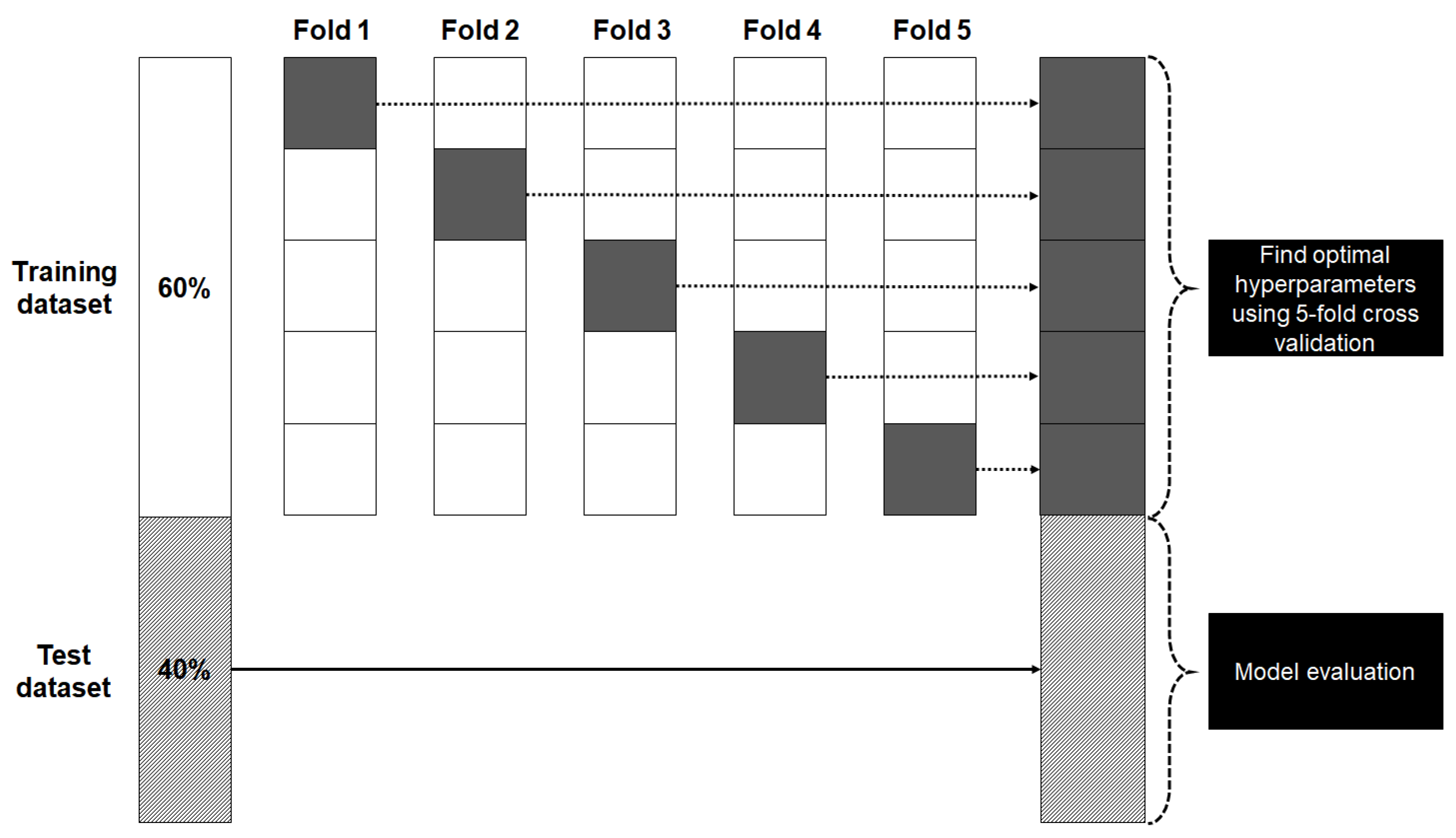
3.1. Machine Learning Approach and Training Process

An RF model was used to classify aerosol type. The RF is an ensemble model based on classification and regression trees (CART), in which multiple trees are aggregated with majority voting and averaged in classification regression tasks [48]. The RF is an enhanced method over individual tree models, which leads to an overfitting problem with a large degree of variability among different data. Breiman [48] suggested an ensemble model based on bagging and randomized node optimization. The RF indicates the importance of each input variable and was used to determine the optimal input variable set that minimized missing data and maximized classification accuracy among various combinations of variable candidates.

The RF model training was carried out using the “randomForest” package (version 4.6-14) [48] in Rstudio (R version 3.6.3, R Studio Inc., Boston, MA, USA). The RF model includes hyperparameters such as ntree (binary classification trees), mtry (the given number of input variables), and node size (the minimum size of terminal nodes). The accuracy of the RF model is reported to depend on these RF hyperparameters so that they would be optimized [48,49]. To determine optimal hyperparameters such as ntree and node size in the RF model, we used the “tune.randomForest” function available from the “e1071” package (version 1.7-3, TU Wien, Vienna, Austria). We attempted to tune model hyperparameters by using node sizes of 1–5 with ntree values of 100–1500. The mtry value was set to the square root of the number of input variables, which is a typical mtry value for classification [50].

The collected dataset was divided randomly into training (60%) and test (40%) datasets. The RF-based model was trained by optimizing hyperparameters based on a k-fold cross-validation procedure. The training dataset was divided randomly into five sets of the same size (Figure 3). The training involved only four folds and was validated with the remaining (unseen) single fold for calculation of model performance. This allowed us to choose optimized hyperparameters that led to the best model performance.

3.2. Classification Model Assessments

3.2.1. Statistical Assessment

In general, classification accuracy can be statistically quantified via confusion matrix analysis [51,52]. Figure 4 shows an example of a confusion matrix, which consists of N columns indicating target classes and N rows for estimated classes. The diagonal terms (e.g., n₁₁, n₂₂, n₃₃, and n_NN) indicate correctly classified instances, whereas off-diagonal terms show incorrectly classified instances. Thus, the confusion matrix provides a measure of classification accuracy as well as insights into misclassification patterns of the classifier. To statistically quantify classification accuracy, we utilized the overall accuracy (OA) and producer’s accuracy (PA) [51,52]. The OA denotes total classification accuracy as the percentage of the number of correctly classified pixels to the total test data (Equation (2)), whereas PA_k represents the classification accuracy of specific class k (Equation (3)).

$$\mathrm{OA}=\frac{{{\displaystyle \sum }}_{k=1}^N{n}_{kk}}{n_{total}}\times 100$$

(2)

$$P{A}_k=\frac{n_{kk}}{n_{k+}}\times 100$$

(3)

where n_total is the total number of test data points, n_kk is the number of pixels correctly classified as class k (diagonal term in the error matrix), and n_k+ is the total number of test data points for specific class k.

3.2.2. Assessment Using AERONET Aerosol Optical Properties

Even though the aerosol type method suggested by Shin et al. [21] is reported to be reasonable for the identification of aerosol sphericity, it was necessary to evaluate the classified aerosol with our RF model using aerosol optical properties from AERONET data. Among several aerosol properties, SSA depends on the complex refractive index (related to extinction coefficient) as well as aerosol size distribution [53,54]. Furthermore, Dubovik et al. [55] also found a wavelength dependency of SSA for each aerosol type. For example, desert dust aerosols show an increasing trend of SSA with increasing wavelength, whereas decreasing SSA values were found with increasing wavelength for biomass-burning smoke aerosols. Therefore, we qualitatively investigated the wavelength dependence of SSA for each aerosol type. In addition, we calculated the differences between several aerosol optical properties (SSA, FMF, and R_d) obtained from AERONET-based aerosol types and RF-based aerosol types.

4. Determination of the Optimal Input Variables

We investigated the contribution of each input variable candidate in our RF-based model to determine the optimal input variable set. To evaluate the importance of each satellite variable by minimizing missing values, we considered three sets of input variable candidates (

Table 2. Summary of variables and data and overall accuracies (OAs) for the initial input variable sets.

Initial Input Variable Sets
Dataset Name	Input Variables	AERONET Data Level	The Number of Data			OA (%)
			Total	Training (60%)	Test (40%)
All input variable candidates (11 variables)	TROPOMI - Aerosol index - Solar zenith angle - CO column amount - Tropospheric NO2 column density MODIS - Aerosol optical depth - Ångström exponent - TOA reflectance at 412, 470 and 660 nm - Land cover type - Percent of urban area	Level 1.5	4906	2946	1960	59%
		Level 2.0	1119	674	445	58%
TROPOMI input variable candidates (4 variables)	- Aerosol index - Solar zenith angle - CO column amount - Tropospheric NO2 column density	Level 1.5	8693	5218	3475	51%
		Level 2.0	1804	1086	718	53%
MODIS input variable candidates (7 variables)	- Aerosol optical depth - Ångström exponent - TOA reflectance at 412, 470 and 660 nm - Land-cover type - Percent of urban area	Level 1.5	5714	3432	2282	56%
		Level 2.0	1348	812	536	52%

):

(1)

All input variable candidates (N = 4906 for Level 1.5 and 1119 for Level 2.0);

(2)

TROPOMI input variable candidates (N = 8693 for Level 1.5 and 1804 for Level 2.0);

(3)

MODIS input variable candidates (N = 5714 for Level 1.5 and 1348 for Level 2.0).

Thus, we investigated classification accuracy and the importance of each input variable to the RF model for these three initial input variable sets.

The OAs of the three initial input variable sets were in the ranges 51–59% and 52–58% for AERONET Level 1.5 and Level 2.0 data, respectively (Table 2). The set of all input variable candidates had the highest OA values of 59% and 58% for Level 1.5 and Level 2.0 data, respectively, indicating the benefit of combining TROPOMI and MODIS data for aerosol identification.

The RF provides the importance of each parameter using the mean decrease accuracy (MDA), which indicates the accuracy lost when a specific variable is excluded from the RF model. Therefore, a variable with a large MDA is more important for the classification algorithm. Figure 5 shows variable importance determined by the RF-based model. TROPOMI-based variables (aerosol index, 83%; SZA, 76%; CO, 70%; NO₂, 64%) have generally higher MDA values than MODIS-based variables except for MODIS AOD. MODIS AOD tends to have a high MDA value of 82%. The TOA reflectance at 660 nm, land cover type, and urban ratio have higher MDA values (>57%) than other MODIS input variables.

Therefore, we chose an optimal input variable set that would assure the highest classification accuracy, while also having high variable importance. All variable candidates from TROPOMI (aerosol index, CO, NO₂, and SZA) and MODIS (AOD, AE, TOA reflectance, land-cover type, and percent urban area) were selected to account for the combined effects of TROPOMI trace-gas data and MODIS aerosol optical properties on aerosol classification (

Table 3. Summary of variables and data points for an optimal input variable set.

Optimal Input Variable Set
Input Variables	AERONET Data Level	The Number of Data			OA (%)
		Total	Training (60%)	Test (40%)
TROPOMI - Aerosol index - Solar zenith angle - CO column amount - Tropospheric NO2 column density MODIS - Aerosol optical depth - Ångström exponent - TOA reflectance at 412, 470 and 660 nm - Land cover type - Percent of urban area	Level 1.5	4906	2946	1960	59%

). The optimal input variable set was constructed using AERONET Level 1.5 data, which can obtain more data than the Level 2.0 data.

5. Results

5.1. Statistical Assessment and Classification Sensitivity of the RF Model

We investigated the confusion matrix and classification accuracy for each aerosol type to determine which type is usually confused or classified well. Aerosol types that are mainly confused with other types were merged based on a sensitivity test via confusion matrix analysis.

When aerosols were classified into seven types (PD, DDM, PDM, SA, MA, WA, and NA), the OA of the RF-based model was 59%. The model generally yielded reliable detection accuracies for the SA (74%), PD (74%), and DDM (69%) types, indicating sensitivity to dust and pollution particles with strong absorption. However, the detection performance for pollution aerosols MA, WA, and NA was generally <47%. The NA type classification accuracy in particular was low (21%). The confusion matrix (Figure 6) indicates that the main confusion occurs between pollution aerosols, apart from the SA type. Pollution aerosols (SA, MA, WA, and NA) tend to be confused with the PDM type in general. Specifically, MA and NA are generally confused with WA. In addition, It turns out our aerosol classifiers have difficulty distinguishing the seven aerosol types with suitable classification performance, especially between the pollution-related aerosols (MA, WA, NA, and PDM). We suggest that it is difficult to discriminate the absorbing features of aerosols in our current model and input variables except for SA aerosols. Furthermore, it is difficult to identify the PDM type that pollution aerosols are slightly mixed with dust aerosols. Thus, the classification performance is expected to be enhanced by merging aerosol classes. Although our model classifies aerosol types with average accuracy of 59%, we tried to additionally improve the performance of our RF-based model by merging aerosol classes. Even though WA class is confused from MA, merging between MA and WA classes may highly decrease the detection accuracy of NA. As a result, the WA type was merged into NA, and MA was integrated into the SA class. Thus, the initial seven aerosol types (PD, DDM, PDM, SA, MA, WA, and NA) were integrated into five aerosol types (PD, DDM, PDM, SA, and NA).

The training process was repeated for the new merged aerosol types. Our RF-based model showed enhanced aerosol detection performance with the OA of 67%. As shown in Figure 7, PAs for each aerosol class of our model ranges from 57% to 77%. In particular, the PA of the NA-type classification is improved greatly, from 21% to 60%. Moreover, there were still good classification performances for SA (77%), PD (75%), and DDM (68%) for our RF-based model. In PDM identification, our model usually confused it with pollution aerosols (NA and SA). The omission error for the PDM classification was found to be mainly caused by SA and NA types (31%), showing that a high contribution of pollution aerosols was responsible for the confusion. It is possible that our RF-based model using satellite variables had insufficient sensitivity to fully detect pollution aerosols that were slightly mixed with dust aerosols. Therefore, we decided to integrate the PDM class into pollution aerosols, so aerosols classified as PDM were reclassified into NA or SA types according to the AERONET SSA value at 1020 nm.

Then, the training process was repeated for the newly merged classes (SA, NA, DDM, and PD). The classification performance was also improved from 67% to 73% (Figure 8). Compared with the seven aerosol types (Figure 6), the new and simplified aerosol classes yielded stable classification performances (68% ≤ PA for each aerosol type classification ≤ 74%). In particular, the PA for NA classification in the RF-based model was greatly improved from 60% to 74%. However, there is still potential for improvement of the classification performance of the RF-based model through the adoption of new satellite input variables and increasing the size of the training dataset. In this section, our RF-based model is found to classify aerosols for up to seven types (PD, DDM, PDM, NA, WA, MA, and SA). The performance of our RF-based model was improved by merging aerosol classes into four (PD, DDM, NA (e.g., sulfate and nitrate), and SA (e.g., carbonaceous aerosols)) resulting in overall accuracy of up to 73%.

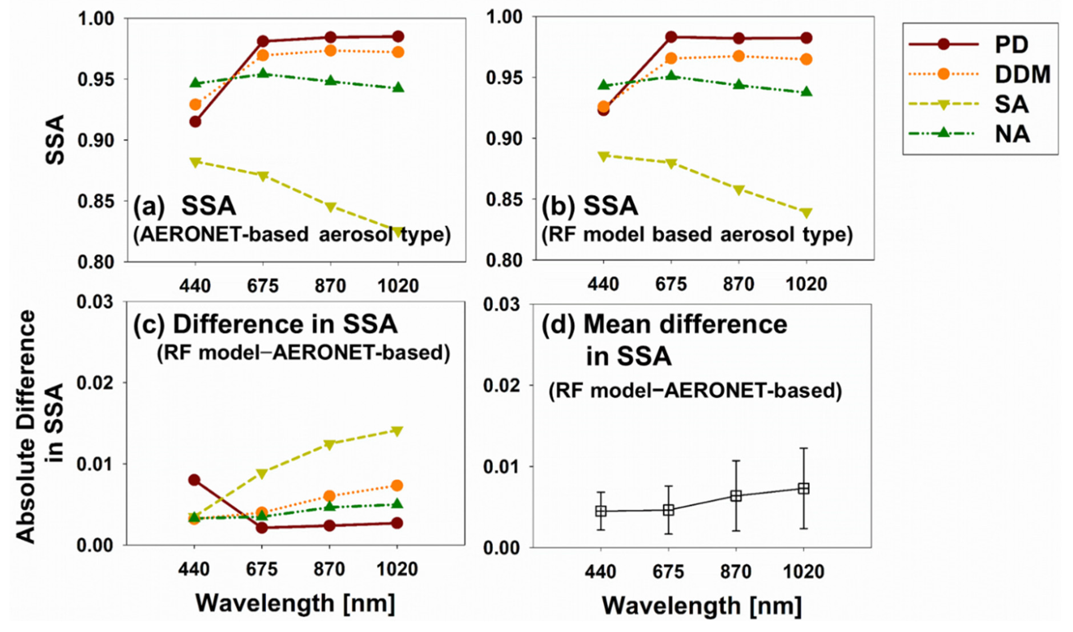
5.2. Evaluation of the RF Model with Aerosol Optical Properties from AERONET Data

The spectral dependence of SSA has been utilized to infer aerosol composition [56]. For example, SSA values of dust aerosols tend to increase with increasing wavelength; however, those of carbonaceous aerosols decrease with increasing wavelength [55,56,57]. As shown in Figure 9a,b, both AERONET-based and RF-based aerosol types showed similar trends in the wavelength dependence of SSA with increasing wavelength for each aerosol type. In particular, the SSAs of PD and DDM tended to increase with wavelength, showing a high contribution of dust aerosols. However, in the case of the DDM type, the increasing rate of SSA with wavelength is lower than that of PD, showing that our RF model was capable of distinguishing PD and dust aerosols slightly mixed with pollution aerosols. In the SA type, SSA values tended to decrease with increasing wavelength, showing that the AERONET-based and our RF-based algorithms reasonably identified the typical wavelength dependence of carbonaceous aerosol types, which is consistent with previous studies [21,55,56,57].

To quantitatively evaluate the performance of our RF-based model using aerosol optical properties for AERONET-based aerosol types, we compared SSA values at several wavelengths (440, 675, 870, and 1020 nm) for AERONET-based aerosol types (Figure 9a) against our RF-based model (Figure 9b). The differences between SSAs for AERONET-based and RF-based aerosol types were calculated (Figure 9c,d). The mean differences in SSA at 440, 675, 870, and 1020 nm were 0.002, 0.004, 0.007, and 0.008, respectively, showing low SSA differences (<0.01 on average).

We also compared the influence of merging aerosol types on the aerosol classification performance in terms of aerosol optical properties, including SSA values at 440, 675, 870, and 1020 nm, FMF, and R_d.

Table 4. Average and standard deviation of differences in SSAs, Fine Mode Fraction (FMF), and R_d for several aerosol classification models, which identifies seven or four aerosol types.

	Seven Aerosol Classes (PD, DDM, PDM, SA, MA, WA, and NA (Sulfate))		Four Aerosol Classes (PD, DDM, SA, and NA (Sulfate))
	Average	Standard Deviation	Average	Standard Deviation
SSA440	0.007	0.006	0.002	0.003
SSA675	0.008	0.009	0.004	0.005
SSA870	0.010	0.011	0.005	0.007
SSA1020	0.012	0.012	0.006	0.008
FMF	0.027	0.020	0.005	0.006
Rd	0.047	0.016	0.016	0.019
Overall accuracy	59%		73%

summarizes the average and standard deviations of differences in SSA values, FMF, and R_d between AERONET-based and RF-based aerosol types. In general, all of these parameters tended to decrease when the aerosol types were merged. For example, with seven aerosol types, differences in SSA at 440, 675, 870, and 1020 nm were 0.007, 0.008, 0.010, and 0.012, respectively, whereas with four aerosol classes, the differences were 0.002, 0.004, 0.005, and 0.006, respectively. The difference in R_d decreased from 0.047 to 0.016 by merging aerosol classes. The difference in R_d also highly decreased the most (0.027 to 0.005) with a decreasing ratio of 81% among other aerosol optical properties. These highly decreasing trends in aerosol optical properties indicate that merging aerosol classes contributed to a decrease in classification confusion in the satellite aerosol classification model.

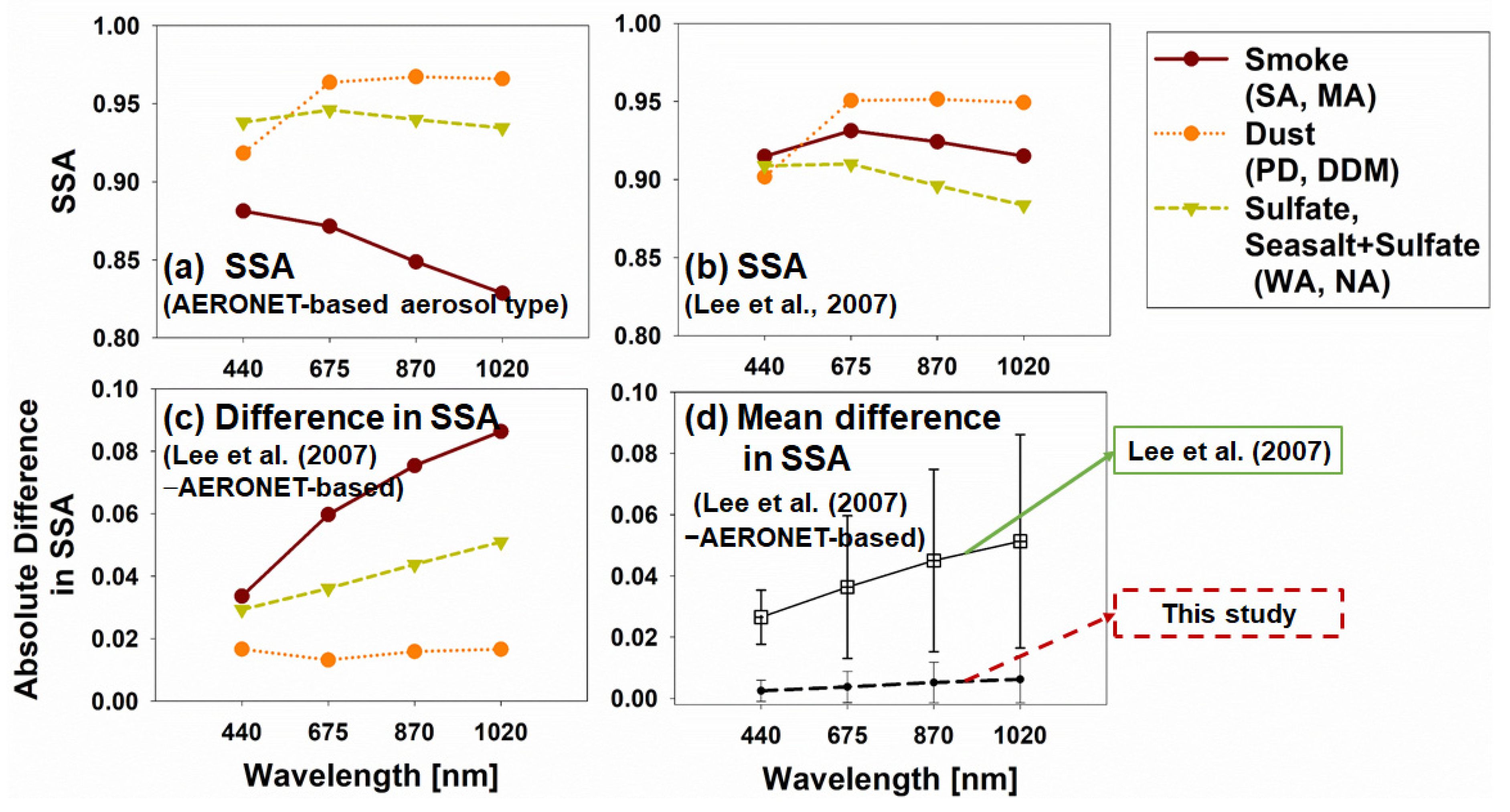
6. Evaluation of the Threshold-Based Aerosol Classification Methods

In this present study, we compared the classification results from earlier aerosol classification methods against those from AERONET-based aerosol classification method [21], which has capability to identify the contribution of non-spherical particles aerosol type. Furthermore, we evaluated the classification methods with aerosol optical properties from the AERONET. The comparison was carried out using the satellite variables from TROPOMI and MODIS measurements data for the period from January 2018 to July 2020 to compare the performance of each aerosol classification algorithm in the same measurement period and with similar data. Two aerosol classification methods have been selected, since they utilize satellite variables that can be obtained from TROPOMI and MODIS [6,8]. The aerosol classification method suggested in Kim et al. [9] has been excluded due to the small number of data points of MODIS FMF. To compare aerosol classification results, we considered the difference in each aerosol classification scheme between earlier aerosol classification methods [6,8] against the AERONET-based aerosol classification method [21].

Table 5. Satellite aerosol classification methods, used input variables, classified aerosol types, and the AERONET-based aerosol types, which have similar aerosol properties.

Method	Variables	Classified Aerosol Types	AERONET-Based Aerosol Types
Lee et al. [8]	Aerosol index AE AOD	Smoke	SA and MA
		Dust	PD and DDM
		Sulfate, Seasalt+Sulfate	WA and NA (sulfate)
		Seasalt	They were not compared due to small number of classified cases (less than 10)
		Dust+Smoke
Torres et al. [6]	Aerosol index CO	Carbonaceous	SA and MA
		Dust	PD and DDM
		Sulfate	WA and NA (sulfate)

summarizes satellite aerosol classification methods, used input variables, classification scheme, and the AERONET-based aerosol types, which have similar aerosol properties. For simplicity, the PDM type was integrated into pollution aerosols (SA, MA, WA, and NA) in the comparison. We compared classification results from earlier satellite methods with AERONET-based aerosol types by calculating the detection rate defined as the satellite/AERONET ratio for each of the classified types with similar aerosol properties (Table 5).

In Lee et al. [8], the aerosol index from OMI and AOD and AE from MODIS are used to classify aerosols. Torres et al. [6] utilized the aerosol index from OMI and CO from AIRS to classify aerosols, whereas in this present study, we used those same products from TROPOMI. As a result of the differences between sensors and retrieval algorithms, thresholds suggested in the previous studies need to be adjusted. In general, TROPOMI aerosol index is found to be less than the OMI aerosol index with a bias within 1 (TROPOMI aerosol index level 2 README Document, 2020). The detection rate was calculated based on various aerosol index thresholds from 0.0 to 1.0. In case of CO, the difference between AIRS CO and TROPOMI CO has not yet been compared. Therefore, the detection rate was calculated under various CO threshold values with the differences of ±5%, ±10%, and ±15%.

Figure 10 shows the detection rates for two threshold-based aerosol classification methods. In general, both aerosol classification methods have very good performance to identify dust aerosols with a detection rate of more than 74% compared with the detection rates of other aerosol types. In the case of Lee et al. [8], the dust detection rate ranges from 78% to 88% under various aerosol index thresholds as shown in Figure 10a. The other aerosol classification algorithm [6] also shows high detection rate ranges from 74% to 100% (Figure 10b). For both aerosol classification methods, the average detection rates tend to increase with decreasing aerosol index threshold. In case of Lee et al. [8], the maximum average detection rate (43%) was found when the aerosol index threshold is 0.1. For Torres et al. [6], highest average detection rate of 55% was found when the aerosol index threshold is 0.1 and the CO threshold is 10% higher than the original CO threshold.

Figure 11 and Figure 12 shows evaluation results between satellite aerosol classification methods against AERONET-based aerosol type using wavelength dependence of SSA. As shown in Figure 10, both aerosol classification methods also showed good agreement between wavelength dependence of SSA for the satellite methods and that for AERONET-based classification method for dust aerosol detection. However, for smoke aerosols detected by Lee et al. [8], we found the highest difference in SSAs compared with other aerosol types (Figure 11c). In general, the wavelength dependence of SSA for smoke and sulfate aerosol appears to be the opposite, indicating a confusion of absorbance for spherical aerosols. The confusion trend between scattering and absorbing properties for spherical aerosols was also observed for the Torres et al. [6] algorithm. The spectral SSA values for smoke and sulfate aerosols detected by Torres et al. [6] were found to be similar compared with those for AERONET-based aerosol types.

7. Discussion

Our newly developed aerosol classification method has an RF-based approach, whereas earlier methods use a threshold-based approach involving input variables from various satellite sensors. Previous studies utilized various satellite input variables including AOD, AE, FMF, aerosol index, and column amounts of trace gases (CO, NO₂, HCHO, and SO₂) from various satellite measurements [3,6,7,8,9,10,11]. Here, we used satellite input variables including AE, AOD, aerosol index, and column amounts of trace gases (tropospheric NO₂ and CO), as suggested in previous studies. In addition, other satellite input variables (SZA, land-cover type, percentage urban area, and TOA reflectance at 412, 470, and 660 nm) were used in the RF-based aerosol classification method.

Aerosol classification methods were evaluated using comparisons between the aerosol climate model and earlier aerosol classification methods [8,9,10]. We evaluated the accuracy of the classification algorithm using the AERONET aerosol-type dataset and typical aerosol property values obtained from AERONET measurements. The overall accuracy of our model for classifying seven aerosol types was 59%, which improved to up to 73% when the seven classes were merged into four aerosol types (PD, DDM, SA, and NA). These four simplified aerosol classes yielded a stable classification performance (68% ≤ PA for each aerosol type classification ≤74%). The typical SSA wavelength dependence for the individual aerosol types is consistent with that determined by our method.

In future studies, the accuracy of the RF model may be improved with more training data being collected over a longer time period. The consideration of more input variables (e.g., meteorological variables) may enhance the sensitivity of aerosol type classification. This study demonstrates that the RF model can classify aerosol types with sensitivity to the contribution of non-spherical particles. Furthermore, the RF-based algorithm has the potential to improve the retrieval accuracy of satellite aerosol and trace-gas algorithms.

8. Summary and Conclusions

In this study, we propose a new method for the identification of aerosol types using an RF model—a machine learning technique. The RF-based model was trained using an AERONET-based aerosol type dataset using MODIS and TROPOMI satellite input-variable datasets. Previous and new satellite input variables were adopted in the RF model, and their importance was investigated. The aerosol index, AOD, SZA, and the column amount of trace gases were found to make substantial contributions to the RF aerosol classification model. The performance of the RF-based model was evaluated using AERONET-based aerosol data and compared with that of previous satellite aerosol classification methods, which use empirically calculated threshold values. Our RF-based model was found to have generally better performance than the previous methods.

Therefore, our RF-based model can identify aerosols of up to seven types, with more aerosol types and greater accuracy than in previous studies that use input variables similar to those of this study. The performance of our RF-based model was improved by merging aerosol classes into four types (PD, DDM, NA [e.g., sulfate and nitrate], and SA [e.g., carbonaceous aerosols]). This merging of aerosol types improved aerosol classification accuracy, with the RF-based method (using satellite variables) having limitations in detailing aerosol compositions. Thus, this study demonstrates that the RF-based model is capable of satellite aerosol classification with a sensitivity to aerosol identification.

With regard to the classification of the sea salt type, this type is not classified in the AERONET-based classification method [21], which was used to construct the AERONET-based aerosol type dataset in this study. Therefore, our current RF-based model does not classify the sea salt type. The sea salt type would be added to the RF-based model if a new AERONET-based aerosol type classification method could classify this type.

References

1. Bréon, F.M.; Goloub, P. Cloud droplet effective radius from spaceborne polarization measurements. Geophys. Res. Lett. 1998, 25, 1879–1882. [Google Scholar] [CrossRef]
2. Charlson, R.J.; Schwartz, S.; Hales, J.; Cess, R.D.; Coakley, J.J.; Hansen, J.; Hofmann, D. Climate forcing by anthropogenic aerosols. Science 1992, 255, 423–430. [Google Scholar] [CrossRef] [PubMed]
3. Higurashi, A.; Nakajima, T. Detection of aerosol types over the East China Sea near Japan from four-channel satellite data. Geophys. Res. lett. 2002, 29, 17-11–17-14. [Google Scholar] [CrossRef]
4. Kaskaoutis, D.; Kambezidis, H. Comparison of the Ångström parameters retrieval in different spectral ranges with the use of different techniques. Meteorol. Atmos. Phys. 2008, 99, 233–246. [Google Scholar] [CrossRef]
5. Remer, L.A.; Kaufman, Y.; Tanré, D.; Mattoo, S.; Chu, D.; Martins, J.V.; Li, R.-R.; Ichoku, C.; Levy, R.; Kleidman, R. The MODIS aerosol algorithm, products, and validation. J. Atmos. Sci. 2005, 62, 947–973. [Google Scholar] [CrossRef] [Green Version]
6. Torres, O.; Ahn, C.; Chen, Z. Improvements to the OMI near-UV aerosol algorithm using A-train CALIOP and AIRS observations. Atmos. Meas. Tech. 2013, 6, 3257–3270. [Google Scholar] [CrossRef] [Green Version]
7. Jeong, M.J.; Li, Z. Quality, compatibility, and synergy analyses of global aerosol products derived from the advanced very high resolution radiometer and Total Ozone Mapping Spectrometer. J. Geophys. Res. Atmos. 2005, 110, D10S08. [Google Scholar] [CrossRef] [Green Version]
8. Lee, J.; Kim, J.; Lee, H.C.; Takemura, T. Classification of aerosol type from MODIS and OMI over East Asia. Asia-Pac. J. Atmos. Sci. 2007, 43, 343–357. [Google Scholar]
9. Kim, J.; Lee, J.; Lee, H.C.; Higurashi, A.; Takemura, T.; Song, C.H. Consistency of the aerosol type classification from satellite remote sensing during the Atmospheric Brown Cloud–East Asia Regional Experiment campaign. J. Geophys. Res. Atmos. 2007, 112, D22S33. [Google Scholar] [CrossRef]
10. Penning de Vries, M.; Beirle, S.; Hörmann, C.; Kaiser, J.; Stammes, P.; Tilstra, L.; Wagner, T. A global aerosol classification algorithm incorporating multiple satellite data sets of aerosol and trace gas abundances. Atmos. Chem. Phys. 2015, 15, 10597–10618. [Google Scholar] [CrossRef] [Green Version]
11. Mao, Q.; Huang, C.; Chen, Q.; Zhang, H.; Yuan, Y. Satellite-based identification of aerosol particle species using a 2D-space aerosol classification model. Atmos. Environ. 2019, 219, 117057. [Google Scholar] [CrossRef]
12. Chu, D.; Kaufman, Y.; Ichoku, C.; Remer, L.; Tanré, D.; Holben, B. Validation of MODIS aerosol optical depth retrieval over land. Geophys. Res. Lett. 2002, 29, MOD2-1–MOD2-4. [Google Scholar] [CrossRef] [Green Version]
13. Qi, Y.; Ge, J.; Huang, J. Spatial and temporal distribution of MODIS and MISR aerosol optical depth over northern China and comparison with AERONET. Chin. Sci. Bull. 2013, 58, 2497–2506. [Google Scholar] [CrossRef] [Green Version]
14. Thrastarson, H.T.; Manning, E.; Kahn, B.; Fetzer, E.; Yue, Q.; Wong, S.; Kalmus, P.; Payne, V.; Olsen, E. AIRS/AMSU/HSB Version 7 Level 2 Product User Guide; Jet Propulsion Laboratory: Pasadena, CA, USA, 2020.
15. Lee, J.; Kim, J.; Song, C.; Kim, S.; Chun, Y.; Sohn, B.; Holben, B. Characteristics of aerosol types from AERONET sunphotometer measurements. Atmos. Environ. 2010, 44, 3110–3117. [Google Scholar] [CrossRef]
16. Russell, P.; Bergstrom, R.; Shinozuka, Y.; Clarke, A.; DeCarlo, P.; Jimenez, J.; Livingston, J.; Redemann, J.; Dubovik, O.; Strawa, A. Absorption Angstrom Exponent in AERONET and related data as an indicator of aerosol composition. Atmos. Chem. Phys. 2010, 10, 1155–1169. [Google Scholar] [CrossRef] [Green Version]
17. Giles, D.M.; Holben, B.N.; Eck, T.F.; Sinyuk, A.; Smirnov, A.; Slutsker, I.; Dickerson, R.; Thompson, A.M.; Schafer, J. An analysis of AERONET aerosol absorption properties and classifications representative of aerosol source regions. J. Geophys. Res. Atmos. 2012, 117, D17203. [Google Scholar] [CrossRef] [Green Version]
18. Giles, D.M.; Holben, B.N.; Eck, T.F.; Smirnov, A.; Sinyuk, A.; Schafer, J.; Sorokin, M.G.; Slutsker, I. Aerosol Robotic Network (AERONET) version 3 aerosol optical depth and inversion products. AGUFM 2017, 2017, A11O-01. [Google Scholar]
19. Zo, I.-S.; Shin, S.-K. A short note on the potential of utilization of spectral AERONET-derived depolarization ratios for aerosol classification. Atmosphere 2019, 10, 143. [Google Scholar] [CrossRef] [Green Version]
20. Noh, Y.; Müller, D.; Lee, K.; Kim, K.; Lee, K.; Shimizu, A.; Sano, I.; Park, C.B. Depolarization ratios retrieved by AERONET sun–sky radiometer data and comparison to depolarization ratios measured with lidar. Atmos. Chem. Phys. 2017, 17, 6271–6290. [Google Scholar] [CrossRef] [Green Version]
21. Shin, S.-K.; Tesche, M.; Noh, Y.; Müller, D. Aerosol-type classification based on AERONET version 3 inversion products. Atmos. Meas. Tech. 2019, 12, 3789–3803. [Google Scholar] [CrossRef] [Green Version]
22. Gupta, P.; Christopher, S.A. Particulate matter air quality assessment using integrated surface, satellite, and meteorological products: 2. A neural network approach. J. Geophys. Res. Atmos. 2009, 114, D14205. [Google Scholar] [CrossRef] [Green Version]
23. You, W.; Zang, Z.; Zhang, L.; Li, Z.; Chen, D.; Zhang, G. Estimating ground-level PM10 concentration in northwestern China using geographically weighted regression based on satellite AOD combined with CALIPSO and MODIS fire count. Remote Sens. Environ. 2015, 168, 276–285. [Google Scholar] [CrossRef]
24. Choubin, B.; Abdolshahnejad, M.; Moradi, E.; Querol, X.; Mosavi, A.; Shamshirband, S.; Ghamisi, P. Spatial hazard assessment of the PM10 using machine learning models in Barcelona, Spain. Sci. Total Environ. 2020, 701, 134474. [Google Scholar] [CrossRef] [PubMed]
25. Park, S.; Shin, M.; Im, J.; Song, C.-K.; Choi, M.; Kim, J.; Lee, S.; Park, R.; Kim, J.; Lee, D.-W.; et al. Estimation of ground-level particulate matter concentrations through the synergistic use of satellite observations and process-based models over South Korea. Atmos. Chem. Phys. 2019, 19, 1097–1113. [Google Scholar] [CrossRef] [Green Version]
26. Park, S.; Lee, J.; Im, J.; Song, C.-K.; Choi, M.; Kim, J.; Lee, S.; Park, R.; Kim, S.-M.; Yoon, J. Estimation of spatially continuous daytime particulate matter concentrations under all sky conditions through the synergistic use of satellite-based AOD and numerical models. Sci. Total Environ. 2020, 713, 136516. [Google Scholar] [CrossRef] [PubMed]
27. Stafoggia, M.; Bellander, T.; Bucci, S.; Davoli, M.; De Hoogh, K.; De’Donato, F.; Gariazzo, C.; Lyapustin, A.; Michelozzi, P.; Renzi, M. Estimation of daily PM10 and PM2. 5 concentrations in Italy, 2013–2015, using a spatiotemporal land-use random-forest model. Environ. Int. 2019, 124, 170–179. [Google Scholar] [CrossRef]
28. Han, H.J.; Sohn, B. Retrieving Asian dust AOT and height from hyperspectral sounder measurements: An artificial neural network approach. J. Geophys. Res. Atmos. 2013, 118, 837–845. [Google Scholar] [CrossRef]
29. Chimot, J.; Veefkind, J.P.; Vlemmix, T.; de Haan, J.F.; Amiridis, V.; Proestakis, E.; Marinou, E.; Levelt, P.F. An exploratory study on the aerosol height retrieval from OMI measurements of the 477 nm O 2-O 2 spectral band using a neural network approach. Atmos.Meas.Tech. 2017, 10, 783. [Google Scholar] [CrossRef] [Green Version]
30. Shimizu, A.; Sugimoto, N.; Matsui, I.; Arao, K.; Uno, I.; Murayama, T.; Kagawa, N.; Aoki, K.; Uchiyama, A.; Yamazaki, A. Continuous observations of Asian dust and other aerosols by polarization lidars in China and Japan during ACE-Asia. J. Geophys. Res. Atmos. 2004, 109, D19S17. [Google Scholar] [CrossRef]
31. Tesche, M.; Ansmann, A.; Müller, D.; Althausen, D.; Engelmann, R.; Freudenthaler, V.; Groß, S. Vertically resolved separation of dust and smoke over Cape Verde using multiwavelength Raman and polarization lidars during Saharan Mineral Dust Experiment 2008. J. Geophys. Res. Atmos. 2009, 114, D13202. [Google Scholar] [CrossRef]
32. Veefkind, J.; Boersma, K.; Wang, J.; Kurosu, T.; Krotkov, N.; Chance, K.; Levelt, P. Global satellite analysis of the relation between aerosols and short-lived trace gases. Atmos. Chem. Phys. 2011, 11, 1255–1267. [Google Scholar] [CrossRef] [Green Version]
33. Lambert, J.; Compernolle, S.; Eichmann, K.; de Graaf, M.; Hubert, D.; Keppens, A.; Kleipool, Q.; Langerock, B.; Sha, M.; Verhoelst, T. Quarterly Validation Report of the Copernicus Sentinel-5 Precursor Operational Data Products# 06: April 2018–February 2020; Belgian Institute for Space Aeronomy: Uccle, Belgium, 2020. [Google Scholar]
34. van Geffen, J.; Eskes, H.; Boersma, K.; Maasakkers, J.; Veefkind, J. TROPOMI ATBD of the Total and Tropospheric NO2 Data Products; KNMI: De Bilt, The Netherlands, 2019. [Google Scholar]
35. Feng, T.; Bei, N.; Zhao, S.; Wu, J.; Li, X.; Zhang, T.; Cao, J.; Zhou, W.; Li, G. Wintertime nitrate formation during haze days in the Guanzhong basin, China: A case study. Environ. Poll. 2018, 243, 1057–1067. [Google Scholar] [CrossRef]
36. Pathak, R.K.; Wu, W.S.; Wang, T. Summertime PM 2.5 ionic species in four major cities of China: Nitrate formation in an ammonia-deficient atmosphere. Atmos. Chem. Phys. 2009, 9, 1711–1722. [Google Scholar] [CrossRef] [Green Version]
37. Zhao, B.; Wang, S.; Liu, H.; Xu, J.; Fu, K.; Klimont, Z.; Hao, J.; He, K.; Cofala, J.; Amann, M. NOx emissions in China: Historical trends and future perspectives. Atmos. Chem. Phys. 2013, 13, 9869–9897. [Google Scholar] [CrossRef] [Green Version]
38. Zhao, Z.-Y.; Cao, F.; Fan, M.-Y.; Zhang, W.-Q.; Zhai, X.-Y.; Wang, Q.; Zhang, Y.-L. Coal and biomass burning as major emissions of NOX in Northeast China: Implication from dual isotopes analysis of fine nitrate aerosols. Atmos. Environ. 2020, 242, 117762. [Google Scholar] [CrossRef]
39. Chen, F.; Lao, Q.; Jia, G.; Chen, C.; Zhu, Q.; Zhou, X. Seasonal variations of nitrate dual isotopes in wet deposition in a tropical city in China. Atmos. Environ. 2019, 196, 1–9. [Google Scholar] [CrossRef]
40. Elliott, E.M.; Kendall, C.; Wankel, S.D.; Burns, D.A.; Boyer, E.; Harlin, K.; Bain, D.J.; Butler, T. Nitrogen isotopes as indicators of NO x source contributions to atmospheric nitrate deposition across the midwestern and northeastern United States. Environ. Sci. Tech. 2007, 41, 7661–7667. [Google Scholar] [CrossRef] [PubMed]
41. Elliott, E.M.; Yu, Z.; Cole, A.S.; Coughlin, J.G. Isotopic advances in understanding reactive nitrogen deposition and atmospheric processing. Sci. Total Environ. 2019, 662, 393–403. [Google Scholar] [CrossRef] [PubMed]
42. Fan, M.-Y.; Zhang, Y.-L.; Lin, Y.-C.; Chang, Y.-H.; Cao, F.; Zhang, W.-Q.; Hu, Y.-B.; Bao, M.-Y.; Liu, X.-Y.; Zhai, X.-Y. Isotope-based source apportionment of nitrogen-containing aerosols: A case study in an industrial city in China. Atmos. Environ. 2019, 212, 96–105. [Google Scholar] [CrossRef]
43. Theys, N.; Smedt, I.D.; Yu, H.; Danckaert, T.; Gent, J.V.; Hörmann, C.; Wagner, T.; Hedelt, P.; Bauer, H.; Romahn, F. Sulfur dioxide retrievals from TROPOMI onboard Sentinel-5 Precursor: Algorithm theoretical basis. Atmos. Meas. Tech. 2017, 10, 119–153. [Google Scholar] [CrossRef] [Green Version]
44. Dickerson, R.; Kondragunta, S.; Stenchikov, G.; Civerolo, K.; Doddridge, B.; Holben, B. The impact of aerosols on solar ultraviolet radiation and photochemical smog. Science 1997, 278, 827–830. [Google Scholar] [CrossRef] [Green Version]
45. Tao, M.; Chen, L.; Wang, Z.; Wang, J.; Che, H.; Xu, X.; Wang, W.; Tao, J.; Zhu, H.; Hou, C. Evaluation of MODIS Deep Blue aerosol algorithm in desert region of East Asia: Ground validation and intercomparison. J. Geophys. Res. Atmos. 2017, 122, 10357–310368. [Google Scholar] [CrossRef]
46. Wu, S.; Mickley, L.J.; Kaplan, J.; Jacob, D.J. Impacts of changes in land use and land cover on atmospheric chemistry and air quality over the 21st century. Atmos. Chem. Phys. 2012, 12, 1597–1609. [Google Scholar] [CrossRef] [Green Version]
47. Fu, Y.; Liao, H. Impacts of land use and land cover changes on biogenic emissions of volatile organic compounds in China from the late 1980s to the mid-2000s: Implications for tropospheric ozone and secondary organic aerosol. Tellus B 2014, 66, 24987. [Google Scholar] [CrossRef]
48. Breiman, L. Random forests. Mach. Learn. 2001, 45, 5–32. [Google Scholar] [CrossRef] [Green Version]
49. Mutanga, O.; Adam, E.; Cho, M.A. High density biomass estimation for wetland vegetation using WorldView-2 imagery and random forest regression algorithm. Int. J. Appl. Earth Obs. 2012, 18, 399–406. [Google Scholar] [CrossRef]
50. Probst, P.; Wright, M.N.; Boulesteix, A.L. Hyperparameters and tuning strategies for random forest. WIREs Data Min. Knowl. 2019, 9, e1301. [Google Scholar] [CrossRef] [Green Version]
51. Jager, G.; Benz, U. Measures of classification accuracy based on fuzzy similarity. IEEE T. Geosci. Remote 2000, 38, 1462–1467. [Google Scholar] [CrossRef]
52. Foody, G.M. Status of land cover classification accuracy assessment. Remote Sens. Environ. 2002, 80, 185–201. [Google Scholar] [CrossRef]
53. Bergstrom, R.W.; Russell, P.B.; Hignett, P. Wavelength dependence of the absorption of black carbon particles: Predictions and results from the TARFOX experiment and implications for the aerosol single scattering albedo. J. Atmos. Sci. 2002, 59, 567–577. [Google Scholar] [CrossRef] [Green Version]
54. Aoki, T.; Tanaka, T.Y.; Uchiyama, A.; Chiba, M.; Mikami, M.; Yabuki, S.; Key, J.R. Sensitivity experiments of direct radiative forcing caused by mineral dust simulated with a chemical transport model. J. Meteorol. Soc. Jpn. 2005, 83, 315–331. [Google Scholar] [CrossRef] [Green Version]
55. Dubovik, O.; Holben, B.; Eck, T.F.; Smirnov, A.; Kaufman, Y.J.; King, M.D.; Tanré, D.; Slutsker, I. Variability of absorption and optical properties of key aerosol types observed in worldwide locations. J. Atmos. Sci. 2002, 59, 590–608. [Google Scholar] [CrossRef]
56. Li, J.; Carlson, B.E.; Lacis, A.A. Using single-scattering albedo spectral curvature to characterize East Asian aerosol mixtures. J. Geophys. Res. Atmos. 2015, 120, 2037–2052. [Google Scholar] [CrossRef]
57. Meloni, D.; Di Sarra, A.; Pace, G.; Monteleone, F. Aerosol optical properties at Lampedusa (Central Mediterranean). 2. Determination of single scattering albedo at two wavelengths for different aerosol types. Atmos. Chem. Phys. 2006, 6, 715–727. [Google Scholar] [CrossRef] [Green Version]
Figure 1. A flow chart of the development of the aerosol classification algorithm based on a machine learning approach.
Remotesensing 13 00609 g001
Figure 2. Spatial distribution of Aerosol Robotic NETwork (AERONET) sites where AERONET (a) Level 1.5 and (b) Level 2.0 data (single-scattering albedo (SSA) and depolarization ratios at 1020 nm) were collected at an overpass time (13:30 LT) of TROPOspheric Monitoring Instrument (TROPOMI) (Sentinel-5P) and Moderate Resolution Imaging Spectroradiometer (MODIS) (Aqua) from January 2018 to July 2020. For Level 1.5, the data where aerosol optical depth (AOD) is higher than 0.4 were only collected.
Remotesensing 13 00609 g002
Figure 3. The schematic diagram of learning process via 5-fold cross-validation procedure and evaluation with test dataset.
Remotesensing 13 00609 g003
Figure 4. Example of a confusion matrix in the estimation of N classes. The term nij denotes the number of instances classified as i by the classifier (estimated class) when they actually belong to class number j (target class). The sums of the confusion matrix elements over rows i and j are represented by ni+ and n+j, respectively.
Remotesensing 13 00609 g004
Figure 5. Variable importance determined by the random forest (RF) model.
Remotesensing 13 00609 g005
Figure 6. Confusion matrix and producer’s accuracy (PA) of each aerosol for the classification of seven aerosol types (pure dust (PD), dust dominant mixed (DDM), pollution dominant mixed (PDM), strongly absorbing (SA), moderately absorbing (MA), weakly absorbing (WA), and non-absorbing (NA; sulfate)).
Remotesensing 13 00609 g006
Figure 7. Confusion matrix and producer’s accuracy (PA) of each aerosol for the classification of five aerosol types (pure dust (PD), dust dominant mixed (DDM), pollution dominant mixed (PDM), strongly absorbing (SA), and non-absorbing (NA; sulfate)).
Remotesensing 13 00609 g007
Figure 8. Confusion matrix and producer’s accuracy (PA) of each aerosol for the classification of four aerosol types (pure dust (PD), dust dominant mixed (DDM), strongly absorbing (SA), and non-absorbing (NA; sulfate)).
Remotesensing 13 00609 g008
Figure 9. Wavelength dependence of SSA at 440, 675, 870, and 1020 nm for (a) AERONET-based aerosol types and (b) RF-based aerosol types, as well as the (c) absolute difference in SSA for each aerosol type and (d) average difference in SSA. Error bars represent the standard deviation of SSA difference.
Remotesensing 13 00609 g009
Figure 10. Detection rates for various thresholds of (a) classified aerosol type by Lee et al. [8] and (b) classified type aerosol by Torres et al. [6]. The detection rate was not calculated in case that the number of data point is less than 10.
Remotesensing 13 00609 g010
Figure 11. Wavelength dependence of SSA at 440, 675, 870, and 1020 nm for (a) AERONET-based aerosol types and (b) Lee et al. [8]-based aerosol types, as well as the (c) absolute difference in SSA for each aerosol type and (d) average difference in SSA. Error bars represent the standard deviation of SSA difference.
Remotesensing 13 00609 g011
Figure 12. Wavelength dependence of SSA at 440, 675, 870, and 1020 nm for (a) AERONET-based aerosol types and (b) Torres et al. [6]-based aerosol types, as well as the (c) absolute difference in SSA for each aerosol type and (d) average difference in SSA. Error bars represent the standard deviation of SSA difference.
Remotesensing 13 00609 g012