Abstract
This article addresses the challenge of 6D aircraft pose estimation from a single RGB image during the flight. Many recent works have shown that keypoints-based approaches, which first detect keypoints and then estimate the 6D pose, achieve remarkable performance. However, it is hard to locate the keypoints precisely in complex weather scenes. In this article, we propose a novel approach, called Pose Estimation with Keypoints and Structures (PEKS), which leverages multiple intermediate representations to estimate the 6D pose. Unlike previous works, our approach simultaneously locates keypoints and structures to recover the pose parameter of aircraft through a Perspective-n-Point Structure (PnPS) algorithm. These representations integrate the local geometric information of the object and the topological relationship between components of the target, which effectively improve the accuracy and robustness of 6D pose estimation. In addition, we contribute a dataset for aircraft pose estimation which consists of 3681 real images and 216,000 rendered images. Extensive experiments on our own aircraft pose dataset and multiple open-access pose datasets (e.g., ObjectNet3D, LineMOD) demonstrate that our proposed method can accurately estimate 6D aircraft pose in various complex weather scenes while achieving the comparative performance with the state-of-the-art pose estimation methods.
1. Introduction
For airborne remote sensing, the accurate pose of the aircraft is very important. However, obtaining the pose just by the inertial devices is not reliable because of the error accumulation. To track this problem, the global navigation satellite system (GNSS) is used as an outer correction to correct the error. However, the GNSS cannot be used in the GPS-denied environment. When the sensors used in the inertial navigation system (INS) fail, it may cause serious consequences, such as the Boeing 737max crash caused by the failure of the angle of attack sensor in recent years. Therefore, it is necessary to design a new aircraft pose estimation method, which can precisely get the pose without using GNSS and INS. In addition, an independent method can also improve the accuracy of pose estimation when it is used with traditional methods. In recent years, with the development of computer vision, vision-based methods have received wide attention, and we decide to tackle this problem by vision-based methods.
As shown in Figure 1, we conduct a system to estimate the aircraft pose in real-time during take-off and landing of the aircraft. This system consists of three parts: the zoom camera subsystem, the pose estimation subsystem, and the servo control subsystem. The zoom camera system captures the 2D image of the aircraft. Then the pose estimation subsystem estimates the 6D pose parameter based on the captured image. Next, the servo control subsystem controls the zoom camera subsystem to capture the next 2D image. The figure of this system is shown in Figure 2. In this article, we focus on the pose estimation subsystem and propose a new algorithm to estimate the aircraft pose quickly, accurately, and robustly.
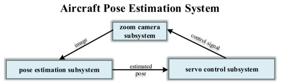
Figure 1.
Illustration of the aircraft pose estimation system. This system consists of three parts: the zoom camera subsystem, the pose estimation subsystem, and the servo control subsystem. The zoom camera system is used to capture the 2D image. The pose estimation subsystem is used to estimate the 6D pose parameter. The servo control subsystem is used to control the zoom camera subsystem.
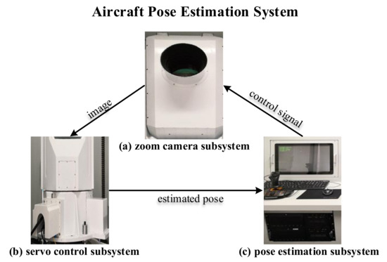
Figure 2.
Figure of the real aircraft pose estimation system. (a) The zoom camera subsystem. (b) The servo control subsystem. (c) The pose estimation subsystem.
Object pose estimation is a challenging task in the field of computer vision. In recent years, researchers have designed many algorithms for different application scenarios, such as robot control, virtual reality, augmented reality. However, there is no specific method or dataset for the aircraft. In this article, we focus on estimating the 6D aircraft pose, i.e., rotation and translation in 3D, from a single RGB image. This problem is quite challenging from many perspectives, such as fog and haze, variations in illumination and appearance, and the atmospheric jitter in the camera imaging process.
Traditionally, object pose estimation using RGB image is tackled by feature- matching [1,2,3] or template-matching [4,5,6,7,8,9]. However, feature-based methods rely heavily on the robustness of features, and they cannot handle texture-less objects. For the template-matching methods, although they can effectively estimate the texture-less objects‘ pose, they cannot handle occlusions between objects very well. With the development of deep learning, many methods use convolutional neural networks (CNNs) to estimate the objects‘ pose. In References [10,11,12,13,14,15,16], researchers train end-to-end neural networks to directly regress the pose, such as viewpoints, quaternions. Refs [17,18] cast the problem of 6D pose estimation as classification into discrete angles. However, these direct methods not only require the networks to learn how to extract pose-related features but also force the networks to learn the complex perspective geometry for recovering the pose parameters directly from the extracted features. In References [19,20,21,22,23,24,25,26,27,28,29], researchers first use CNNs to locate 2D keypoints and then recover the pose parameters using the Perspective-n-Point (PnP) algorithms. These two-stages methods use keypoints as the intermediate representations to indirectly estimate the 6D pose, which makes networks focus on learning how to extract features related to keypoints, without considering the complex perspective geometry. Thus, these methods achieve state-of-the-art performance. Inspired by these keypoint-based methods, HybridPose [30] uses keypoints, edge, and symmetry correspondences to recover the 6D pose and achieve remarkable performance. However, the edge vectors are defined between the adjacent keypoints which means edge vectors and keypoints are not independent of each other.
There are complex and changeable weather scenes during the aircraft flight. As shown in Figure 3, when the weather is good, the aircraft in the image is clear and the keypoints can be predicted precisely. However, when the weather is bad, it is hard to locate the keypoints. Severe fog, haze, and atmospheric jitter blur the aircraft in the image, as a result, the keypoints cannot be precisely located. In addition, over exposure causes dramatic changes in the aircraft appearance and even a lack of texture information, making it more difficult to locate the keypoints. Therefore, these methods which just rely on keypoints as the intermediate representations may fail in complex weather scenes.
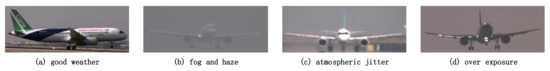
Figure 3.
Complex weather scenes during the aircraft flight. As shown in (a), the weather is good, and the aircraft in the image is clear. As shown in (b), severe fog and haze blur the aircraft in the image. As shown in (c), the atmospheric jitter in the camera imaging process makes it hard to recognize the keypoints precisely. As shown in (d), over exposure causes a lack of texture information.
In this article, we introduce Pose Estimation with Keypoints and Structures (PEKS), a novel 6D pose estimation method that leverages multiple intermediate representations to express the geometric information of target. Except for the conventional keypoints, PEKS simultaneously utilizes the CNN to output geometric structures for reflecting each part of target and its topological relationship. This type of representation has the following advantages. First, it integrates more information of the target. As a kind of local geometric feature, keypoints represent the points with rich geometric information while structures encode the geometric relationship between different parts of the object globally. Second, it improves the accuracy of pose estimation when the weather is poor with the help of the robustness of structures to illumination and blurring. Third, it can be shown that training the keypoints and structures jointly achieve better results than training separately. We select 17 points with rich geometric information as keypoints and define the structures as six line segments which represent the fuselage and plane wings separately.
Given the predicted keypoints and structures, the next step is to estimate the 6D pose by these representations. Previous approaches recover the 6D pose by PnP algorithms, such as EPNP, OPNP and DLT [31,32,33]. However, the PNP algorithms only work when the input is a set of points and they are not suitable for line segments. To this end, we extend the optimization objective of traditional PNP algorithms to make it applicable for line segments. To be specific, we represent a line segment by a point which is on it and its direction vector. The extended optimization objective can be deduced according to the theory of multi-view.
We also collect a new dataset for aircraft pose estimation which consists of two parts, one is the real data, containing 3681 images, and the other is the rendered data, containing 216,000 images. The real data are sampled from the aircraft flight videos under different pose and weather scenes. We evaluate our approach mainly on this dataset and it exhibits great performances.
In summary, our work has the following contributions:
- We propose a novel approach for aircraft pose estimation. This approach combines the keypoints and geometric structures as the intermediate representations to estimate the 6D pose in complex weather scenes.
- We propose a PnPS algorithm, which recovers the 6D pose parameters based on predicted keypoints and structures.
- We contribute a dataset for 6D aircraft pose estimation, which consists of 3681 real images and 21,6000 rendered images.
The rest of this article is organized as follows. We review the related work in Section 2. In Section 3, we present the detailed architecture of our approach. In Section 4, we describe the datasets and metrics while Section 5 discusses the settings and experiments. Finally, the conclusion with future work is given in Section 6.
2. Related Work
Methods for 6D object pose estimation from a single RGB image in the literature can be roughly classified into classical methods and CNN-based methods. In this section, we give a brief introduction to them.
2.1. Classical Methods
In classical methods, local features or templates are used to estimate the 6D pose. In feature-based methods [1,2,3,33,34], local features are first extracted and the matched to 3D models for establishing the 2D-3D correspondences; thus, the 6D pose can be estimated steadily. Features such as SIFT, SURF and ORB [34,35,36] are widely used in these methods which are robust to illumination, scale, and rotation. A drawback of these methods is that they are inadequate for addressing texture-less objects and their performance is susceptible to scene clutter. In template-based methods [4,5,6,7,8,9], templates are constructed by rendering the model of objects from different poses. Then these templates are matched against the input image to determine the object pose in the image. Template-based methods are useful for texture-less objects. However, they cannot handle occlusions between objects very well. When the object is heavily occluded, the matching score is low which causes incorrect pose estimation results.
2.2. CNN-Based Methods
With the development of deep learning, researchers begin to tackle the task of 6D pose estimation by CNNs. In References [10,11,12,13,14,16], researchers train an end-to-end CNN to directly regress the 6D pose. PoseNet [37] uses CNN to directly regress the pose of the camera, which is similar to object pose estimation. Refs [17,18] discretize the 6D pose space and cast the problem of 6D pose estimation as classification. Ref [13] trains the end-to-end CNN by means of self-supervised learning. Ref [14] directly regresses 6D poses from correspondences of 2D-3D points without PnP algorithm. However, these methods force the networks to learn the complex perspective geometry to recover the pose parameters directly from the extracted features which increases the difficulty of training.
With the development of perspective geometry, we can recover the pose parameters by Perspective-n-Point (PnP) algorithm and what we only need to know is the 2D-3D correspondences of keypoints. This casts the problem of 6D pose estimation as locating keypoints and many keypoint-based methods [19,20,21,22,23,24,25,26,27,28,29] are proposed in recent years. These methods adopt a two-stage pipeline: they first use CNNs to locate the designed 2D keypoints and then recover the pose parameters using the PnP algorithm. In other words, these methods use keypoints as intermediate representations to indirectly estimate the 6D pose, which makes networks focus on learning how to extract features related to keypoints, without considering the complex perspective geometry. SSD-6D [19] employs the SSD architecture to locate the 8 corners of the 3D bounding box and the center of the object. Similarly, ref [20] employs the YOLO architecture to locate these nine keypoints. However, the 8 corners of the 3D bounding box are far away from the object pixels and are easily interfered with the background which results in large localization errors. Ref [22] replaces these 8 corners with keypoints on the surface of the object selected by the 3D-SIFT algorithm [38]. PVNet [21] uses a pixel-wise voting network to locate the keypoints which are selected by the farthest point sampling algorithm from the object surface. Furthermore, hybridPose utilizes a hybrid intermediate representation to express different geometric information in the input image, including keypoints, edge vectors, and symmetry correspondences.
Pose estimation methods are also widely used in unmanned autonomous vehicles. Inspired by the recent success of deep learning, CodeSLAM [39] employs a neural network to learn a compact latent representation for the structure of a scene conditioned on the RGB image and achieved remarkable performance. KDP-SLAM [40] combines photometric and geometric loss for frame-to-frame pose estimation. Probabilistic-VO [41] combines points together with lines and planes for pose estimation while considering their uncertainties.
Deep learning methods have dominated human pose estimation tasks in recent years and achieved remarkable performance [22,23]. The core of human pose estimation is how to precisely predict the pixel location of important keypoints of the human body which is similar to the keypoints based methods. Therefore, these methods are instructive to the task of object pose estimation. Ref [23] locates the keypoints of indoor objects by Stacked Hourglass Networks [42]. Reference [43] employs the Convolutional Pose Machine [44] to estimate the object pose by locating the keypoints.
Inspired by these methods, we propose a novel two-stage approach for aircraft pose estimation which locates the keypoints and structures of the aircraft by a CNN and then recovers the 6D pose parameters by a PnPS algorithm.
3. Methodology
The major challenge of aircraft pose estimation comes from the complex weather scenes during the flight, such as severe fog and haze, atmospheric jitter, and over exposure. Targeting to overcome those challenges, we propose a novel approach for aircraft pose estimation. Given an image, the task of aircraft pose estimation is to estimate the aircraft’s rotation and translation in 3D. Specifically, the 6D aircraft pose is represented by 3D rotation () and 3D translation () from the aircraft coordinate system to the camera coordinate system.
As illustrated in Figure 4, we estimate the aircraft pose using a two-stage pipeline: we first predict geometric features of the aircraft which serve as intermediate representations and then recover the 6D pose parameters by the PnPS algorithm. Our innovations are the new intermediate representations for pose estimation which combine the keypoints and structures, as well as the PnPS algorithm.
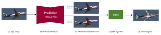
Figure 4.
Pipeline of our approach. Given a single RGB image of an aircraft (a), we utilize prediction networks (b) to locate the keypoints (red points) and structures (red structures) which serve as intermediate representation (c). Then the 6D pose is estimated by the PnPS algorithm (d) based on the predicted results (e).
As illustrated in Figure 5, PEKS consists of a CNN block, a predictor block, and a pose solve block. The CNN block utilizes a encoder and decoder structure to generate a set of heatmaps of keypoints and a set of heatmaps of structures . Then the predictor block predicts a set of keypoints and a set of structures based on the generated heatmaps. and are all expressed in 2D. In the following, we denote 3D keypoint coordinates in the world coordinate system as , where K is the number of keypoints. We denote the 3D structures in the camera coordinate system as , where S is the number of structures. To make notations uncluttered, we denote the predicted keypoints as and predicted structures as . The pose solve block optimizes the pose to fit the intermediate representations by the PnPS algorithm.
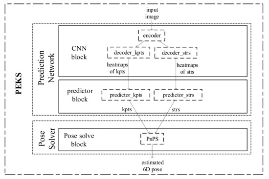
Figure 5.
Block diagram of our approach. Given a single RGB image of an aircraft, we utilize a CNN block to generate the heatmaps of the intermediate representation which are keypoints and structures. Then a predictor block is employed to predict the keypoints and structures. The 6D pose parameters are estimated by the pose solve block by the PnPS algorithm. For convenience, we denote keypoints as kpts and structures as strs in this figure.
3.1. Locate Keypoints and Structures
3.1.1. Keypoints Definition
The intermediate representations need to be defined based on the 3D aircraft model. The first intermediate representation consists of keypoints , which have been widely used for pose estimation. Refs [19,20,45] use the eight corners of the 3D bounding box as the keypoints which are far away from the object pixels and are easily interfered with the background. Reference [22] selects keypoints from the surface of the object by 3D-SIFT algorithm while Reference [21] by the farthest point sampling algorithm. However, simply selecting keypoints from the aircraft surface through algorithms is unreliable because of the complex weather scenes. Severe fog and atmospheric jitter blur the aircraft in the image and the over exposure causes huge changes in the aircraft appearance and even leads to a lack of texture information. To reduce the impact of the weather scenes, we select 17 points with rich geometric information rather than texture information from the aircraft surface as keypoints. As shown in Figure 6, the selected keypoints are the apex of the aircraft nose (1 point), the leftmost and the rightmost points of the flight compartment windows (2 points), the tip of the left and right wings (2 points), the vertexes of two horizontal tails (8 points), and the vertexes of the vertical tail (4 points). The reason why we do not select some other points, such as the points on the trailing edge, is that the positions of these points change during the aircraft flight although these points have rich geometric information.
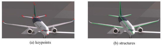
Figure 6.
Keypoints and structures definition. As shown in (a), 17 points on the aircraft surface are defined as keypoints. In (b), six segments which characterize the geometric relationship between different parts of the aircraft are defined as structures.
3.1.2. Structures Definition
The second intermediate representations consist of structures. Reference [46] defines the lines that represent the fuselage and the wings as the structures of the straight-wing UAV which are simple and effective. However, we cannot estimate the pose parameters just by them because cannot be calculated. HybridPose [30] uses edge vectors to capture correlations between keypoints and reveal the underlying structure of the object. However, the edge vectors are defined between the adjacent keypoints which means edge vectors and keypoints are not independent of each other. As shown in Figure 7, the aircraft is mainly composed of six parts which are the fuselage, the left and right wings, the left, and right horizontal tails, and the vertical tail. Based on the idea that each structure corresponds to a part, we select six line segments to represent the topological structure of the aircraft. The defined structures are shown in Figure 6.
Figure 7.
The six parts of an aircraft: fuselage, the left and right wings, the left and right horizontal tails, and the vertical tail.
3.1.3. Locate Keypoints
As shown in Figure 8, the proposed network is a multi-stage architecture with intermediate loss functions after each stage and it is similar to the Stacked Hourglass Networks which is used to locate the keypoints of humans. A cropped image is fed to the network and two hourglass components are used to generate heatmaps for each keypoints. The intensity of the heatmaps indicates the probability of the respective keypoints to be located at every pixel. As shown in Figure 9, each hourglass component first uses residual and max-pooling layers to process features down to a very low resolution. At each max pooling step, the resolution of the feature maps decreases by two. After reaching the lowest resolution, the hourglass component begins to up-sample and combines the features across multiple scales. At each up-sampling layer, the resolution of feature maps increases by two. After reaching the output resolution of the network, one residual layer and two convolutional layers are applied to produce the heatmaps of keypoints. The second hourglass component is stacked to the end of the first to refine the predicted heatmaps. The input of the second one consists of three parts: the input of the first one, the feature maps extracted by the first one, and the heatmaps predicted by the first one.
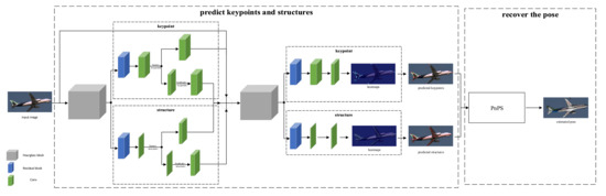
Figure 8.
Detailed architecture of the proposed method. The CNN predicts the keypoints and structures jointly by a two-stage architecture. In the first stage of the network, the heatmaps of keypoints and structures are predicted for intermediate supervision. In the second stage, the features and heatmaps of the first stage after merged is used as input. The final outputs of the network are heatmaps predicted by the second stage. At each stage, an MSE loss is used which compared the predicted heatmaps to the ground-truth heatmaps. After that, a PnPS algorithm is used to recover the 6D pose based on the predicted keypoints and structures.
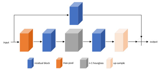
Figure 9.
The detailed architecture of n-hourglass block. The n-hourglass block consists of residual, max-pooling, up-sampling, and n-1 hourglass layers.
Assuming we have K ground-truth heatmaps for a training sample, an MSE loss is applied to compare the predicted heatmaps to the ground-truth heatmaps. The ground-truth heatmaps define the position of keypoints subjects to 2D Gaussian distribution. The loss of keypoints is given by
where x denotes a training sample, denotes the ground-truth heatmap for x, denotes the i-th predicted heatmap. The MSE loss is computed over all pixels in the heatmap, and we write instead of for the MSE loss.
What is more, intermediate supervision is applied at the end of the first component, which can provide a richer gradient to the first hourglass component and guide the learning procedure towards a better optimum. For each predicted heatmap, we consider the pixel with the maximum probability as the location of the keypoint. The value of this pixel is regarded as the confidence of this keypoint.
3.1.4. Locate Structures
As shown in Figure 8, the proposed network not only predicts the keypoints but also the structures. As shown in Section 4, locating the keypoints and structures simultaneously can significantly improve the accuracy of pose estimation when the weather is good. When the weather is bad, the pose can also be estimated accurately by the combination of these two kinds of geometric features, while it is not possible just by locating keypoints. Similar to keypoints, we locate structures by predicting heatmaps of them. A new branch is applied for locating structures, which consists of a residual layer and two convolutional layers.
Assuming we have S ground-truth heatmaps for a training sample, an MSE loss is applied to compare the predicted heatmaps to the ground-truth heatmaps. The ground-truth heatmaps define the positions of structures subject to Gaussian distribution. To be specific, the probability function , returns a probability value for each pixel denoted by e based on its distance to the structures. Formally, we define the probability function as follows:
the distance function is defined as the distance from pixels to structures. Similar to keypoints, the loss of structures is given by
where denotes the ith predicted heatmap of structures. For each heatmap, we fit the structure by the least square method. We first select pixels with values bigger than a certain threshold, then we use the least square method to recover the fittest structure. The reciprocal of the mean distance from pixels to the recovered segment is the confidence of the structure.
In addition, locating the keypoints and structure simultaneously can significantly improve the accuracy of pose estimation regardless of the weather scenes. When the two tasks are trained together, the multi-task loss for the network is then expressed as:
3.2. PnPS Algorithm
Given the keypoints’ locations in the 2D image as well as their correspondences on the 3D model, one approach is to apply the PnP algorithm to solve the 6D pose parameters, such as DLT, EPNP. However, we not only have the 2D-3D correspondences of keypoints but also the 2D-3D correspondences of structures, and existing PnP algorithms are designed only for keypoints. Inspired by the PnP [31,32,33] and PNL [47] algorithms, we propose a new algorithm that can recover the 6D pose parameters based on keypoints and structures.
For keypoints, the basic idea of PnP algorithms is to minimize the reprojection error:
where is the estimated coordinate of the keypoint, is the 3D coordinate of the keypoint, is the 2D projection of , and is the perspective projection function.
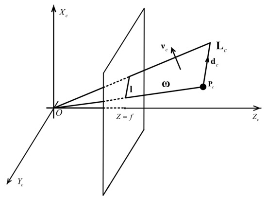
For structure , we represent it by a point which is on it and its direction vector :
As shown in Figure 10, represents the structure in the camera coordinate system, represents the projection of the structure, and is the projection plane while is the normal vector of . Assuming the camera calibration matrix is known, the plane can be expressed as:
and can be calculated from the equation of the plane, which can be represented as:
In addition, is perpendicular to :
According to the rigid transformation from the object coordinate system to camera coordinate system, can be expressed as:
where represents the rigid transformation from the object coordinate system to the camera coordinate system, represents the structure in object coordinate system. The orthogonality relationship can be expressed as:
The optimization objective for structures is:
We also take the confidence of keypoints and structures into account. Similar to Reference [24], we naturally multiply the confidence of the keypoints and structures to the reprojection error, and the final optimization objective is:
where c represents the confidence calculated by heatmaps.
4. Material
4.1. Dataset
4.1.1. Aircraft-Pose-Estimation Dataset
In this article, we introduce a new dataset especially for aircraft pose estimation which contains 3681 real images and 216,000 rendered images, called the APE dataset. All the images in this dataset have the size 1920 × 1080. The dataset contains most kinds of scenes that the aircraft may encounter during flight and can effectively evaluate the robustness of the methods for aircraft pose estimation. For real images, we sampled them from 79 videos captured by our cameras at different airports. These images are under different poses, such as taking off, landing, hovering, taxiing, and different weather scenes. The annotations include the focal and the pixel size of the camera, the 2D bounding box, the 6D pose, the projection of the 3D bounding box, the projection of the keypoints, the projection of the structures, and the weather scenes. We divide the images into four categories according to the weather: good weather, fog and haze, atmospheric jitter, and over exposure. Examples of real images are illustrated in Figure 11. What is more, we also generated 21,6000 rendered images for training. The rendered images were created by placing the 3D aircraft model in front of background images with the help of OpenGL. Background images were chosen from the sky images took manually under different weather scenes and road images from the KITTI dataset [48] which simulate the scenes when the aircraft is hovering in the sky and taxiing on the ground. Examples of rendered images are illustrated in Figure 11. On this dataset, we randomly select 80% of examples for training, 50 instances for validation, and the rest for testing.
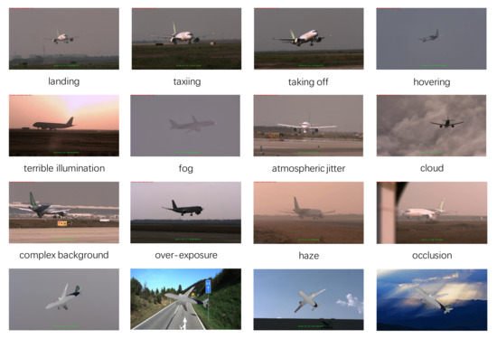
Figure 11.
Examples of images in the APE dataset. The first three rows are real images which are under different pose and weather scenes. The fourth row is rendered images which are under different pose and backgrounds.
4.1.2. ObjectNet3D
To verify the generalization of our model, we test PEKS on this dataset. OBJECTNET-3D [49] is a large dataset that contains real images of 100 object categories. From all of them, we simply select images which class is airplane to evaluate our model. The selected subset contains 1013 images which include not only the manually annotated keypoints but also the viewpoints from aligned 3D shapes. For keypoints, we use these annotations as ground-truth. However, the structures cannot be reprojected from the annotated viewpoints because of the inaccuracy of the 3D shapes. Instead, we annotated the structures manually. On this dataset, we do not fine-tune our model, and all the 1013 images are used for testing.
4.1.3. LineMOD
The LineMOD dataset [50] is one of the standard datasets for 6D pose estimation. It consists of 13 sequences, which contain ground-truth poses for a single object of interest in a cluttered environment and the accurate CAD models. The ground-truth keypoints and structures can be obtained through reprojection according to the annotated poses and the CAD models. Different from other literature, we selected just five sequences to evaluate our algorithm which are cat, lamp, bench vise, cam, and driller. For other objects, their structures are not obvious and our algorithm is not suitable for them. On this dataset, we randomly select 80% of examples for training, 20 instances for validation, and the rest for testing.
4.2. Evaluation Metrics
We evaluate our method using five common metrics: Percentage of Correct Keypoints (PCK) [43], Percentage of Correct Structures (PCS), 2D reprojection metric [24], ADD(-S) metric [50], and and metric [43].
PCK—This metric computes the percentage of keypoints that fall within a normalized Euclidean distance of the corresponding ground-truth. An estimated keypoint is valid if the distance is below , where and are the width and height of the object’s bounding box, respectively.
PCS—To evaluate the accuracy of the estimated structures, we proposed a new metric on the base of the PCK. An estimated structure is valid if the distance with respect to the corresponding ground-truth is below . The distance between two structures is defined as follow:
where and are the start point and the end point of the structure.
2D reprojection metric—This metric computes the mean Euclidean distance between the projections of 3D vertices given by the ground-truth pose and the estimated pose. Formally,
where M is the set of model vertices, and are the ground-truth rotation matrices and translation matrices, and are the predicted ones, and is the camera calibration matrix.
ADD(-S) metric—This metric computes the mean 3D distance between the model vertices transformed by the ground-truth pose and the estimated pose. Formally,
To handle the symmetric objects, the ADD metric can be extended as follow:
which computes the mean 3D distance between the closest vertex of the model transformed by the estimated pose with the ground-truth transformation.
and metric—This metric computes the rotation error and translation error between the predict pose and the ground-truth pose. Formally,
5. Experimental Results and Discussion
In this section, we first give the details of the experiment, then we evaluate the performance of our method, and compare it with several popular pose estimation algorithms. Section 5.1 gives the detailed description of the experiments. Section 5.2 quantitatively and qualitatively evaluate PEKS. Section 5.3 compares PEKS with other pose estimation methods. Section 5.4 analyzes the effectiveness of PEKS.
5.1. Experiments Detail
There are keypoints and structures for the target, PEKS takes the as input, and outputs the tensor representing the heatmaps of keypoints and tensor representing the heatmaps of structures. The location and the confidence of keypoints and structures can be calculated from the heatmaps. The 6D pose is then estimated by the PnPS algorithm. The CNN architecture is implemented with Pytorch 1.2.0 and CUDA 10.0 and runs on an i5-10400 CPU @2.90Ghz with an NVIDIA Geforce RTX 2080Ti. The PnPS algorithm is implemented with Python using Numpy and OpenCV.
5.1.1. Training Setting
We train keypoints and structures using MSE loss as discussed in Section 3. We first train our model on synthetic data using stochastic gradient descent for optimization, with the learning rate initially set as 0.001 and divided by 10 after every 10,000 iterations. Then we train our model on the real data with freezing the hourglass layers and the learning rate initially set as 0.00025 and divide by 10 every 4000 iterations. The batch contains 32 samples per iteration which are sampled randomly. and in Equation (4) are set to 1 and 0.5, respectively.
5.1.2. Data Augmentation
The accuracies of the bounding box in different poses are different which would draw to an error in keypoints and structures location. Therefore, we do a bounding box augmentation in bias and scale with the limitation that the targets are all within the bounding box. What is more, we also apply data augmentation including rotation, scaling, and color jittering in training. We avoid flipping the image horizontally because it may cause a strange geometric relationship between keypoints and structures and confuse the network. Take the aircraft as an example, as shown in Figure 12, in the original image, the tip of the right-wing (number 4) is in the left half of the image, however, in the flipped image, this keypoint is in the right half of the image which should be the tip of the left-wing from the perspective of the model. The reason for this confusion is that mirroring the image causes the 3D model mirrored which puzzles the network by the two similar models. A similar situation exists in the structures.
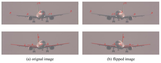
Figure 12.
Flipping the image horizontally may cause confusion. Original image (a) and flipped image (b).
5.2. Qualitative and Quantitative Results of Airplane Pose Estimation
We conduct experiments on the APE dataset to evaluate the performance of our method.
As shown in Table 1, we first evaluate our method in terms of the 2D reprojection metric. A pose is considered correct if the average of the 2D distances is less than 20 pixels. The reason why the threshold value is 20 instead of 5 is that we calculate the 2D reprojection error under the size of . Under this metric, PEKS can estimate the pose parameters precisely and achieve 95.6% accuracy in total. When the weather is good, PEKS can even reach 98.3% accuracy. When the weather scene is terrible, although the accuracy of the algorithm decreases, it still has a correct rate of more than 90%, which shows the robustness and accuracy of the algorithm. When over exposure occurred during camera imaging, the aircraft appearance changes dramatically, and some texture information is hard to extract. However, PEKS still achieves 95.8% accuracy, which thanks to our selection of keypoints with rich geometric information rather than keypoints with texture information. When the weather scene is fog and haze, the aircraft in the image is blurred, and the situation is more serious when atmospheric jitter occurred. Our method still can reach 91.3% and 90.2% accuracy with the help of structures which reflect the topology of the aircraft and robustness to these scenes.

Table 1.
Qualitative result of Pose Estimation with Keypoints and Structures (PEKS) on APE dataset under different metrics.
Then we evaluate our method in terms of the ADD metric. A pose is considered correct if the average of the 3D distance is less than 10% of the aircraft’s size. In this experiment, the size of the aircraft is about 34.8 m, so the threshold of ADD metric is 3.48 m. Under this metric, PEKS can reach 72.7% accuracy in total, which is much less than the results under 2D reprojection metric. As shown in Table 3, the state-of-the-art methods even get worse results. However, this does not mean our method cannot estimate the pose parameters accurately. We analyze the reasons why these algorithms failed on this dataset and find that the ground-truth and the focal of the image in the APE dataset are much bigger than the benchmark datasets. For the APE dataset, during the flight of the aircraft, the distance between the camera and the aircraft varies greatly, and the ground-truth ranges from 100 m to about 5 km. While in other benchmark datasets, take the LineMOD dataset for example, ground-truth is about 1 m. It is unreasonable to evaluate the accuracy of the algorithm with a threshold of 10% of the model’s size. In addition, a zoom lens camera was used to capture the aircraft clearly during the flight, and the focal ranges from 30 mm to 1000 mm. While in other benchmarks, also take the LineMOD dataset for example, the focal is no more than 100 mm. The long focal makes it difficult to accurately estimate pose parameters especially the .
The perspective projection geometry during the imaging process is shown as follows,
where and are the coordinates in the image coordinate system, X,Y,Z are the coordinates in the camera coordinate system, is the focal of the camera. Equation (19) shows that even a small location error may cause a great error for when the focal is long. In other words, the effect of is reduced by the focal because of the perspective projection geometry. Therefore, it is hard to estimate precisely even with the accurate location of intermediate representations when the focal is long. The terrible results of our method on APE dataset in terms of ADD metric are understandable. In addition, the inaccuracy of it does not mean that our network cannot locate the keypoints and structures precisely which can be proved by the results under 2D reprojection metric.
To ignore the effect of and focal, we evaluate our method in terms of metric. A pose is considered correct if the rotation error is less than . Similiar with results under 2D reprojection metric, PEKS can estimate the pose parameters precisely and achieve 95.2% accuracy in total. When the weather scene is good, PEKS reaches 98.2% accuracy. When the weather scene is fog and haze, PEKS reaches 90.7% accuracy. When over exposure and atmospheric jitter occurred, PEKS can still estimate the rotation precisely with an accuracy of 95.3% and 89.2%, respectively.
Figure 13 shows some qualitative results on APE dataset where the yellow points are the keypoints and the purple segments are the structures predicted by the networks. The first line of images is captured under good weather, the second line is under severe fog and haze, the third line is under atmospheric jitter, and the final line is under over exposure. Even the weather is bad our method robustly predicts the keypoints and structures.
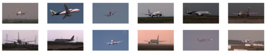
Figure 13.
Qualitative results for the proposed method on the APE dataset. The yellow points are the keypoints and the purple segments are the structures.
5.3. Comparisons with State-of-the-Art Methods
5.3.1. Performance on the APE Dataset
We first compare our method with the state-of-the-art methods on the APE dataset. To compare PEKS with them, we re-implement the same pipeline as [20,25], both of which estimate the 6D pose by regressing the eight corners of the 3D bounding box.
In Table 2, we compare our method with Bb8 [25] and YOLO-6D [20] in terms of the 2D reprojection metric. Bb8 and YOLO-6D choose the eight corners of the 3D bounding box and the center of the aircraft as keypoints and locate them by regression while our method locates the keypoints and structures by predicting their heatmaps. As shown in Table 2, our method outperforms them by 10.8% and 6.3%, respectively. When the weather is good, both YOLO-6D and our methods achieve great results. However, when the weather is bad, the accuracy of Bb8 and YOLO-6D drops significantly, while our method still works well. The reason why Bb8 and YOLO-6D fail when the weather is bad is that the eight corners of the 3D bounding box cannot locate precisely and estimating the 6D pose by the PnP algorithm with keypoints that have large location error is not reliable. In the contrast, although the accuracy is lower than under good weather, our method still works well thanks to the combination of keypoints and geometric structures.
Table 2.
Comparison with the state-of-the-art methods in terms of the 2D reprojection metric on APE dataset. Bold number indicates the best results.
As shown in Table 3, both the state-of-the-art methods and our method work badly in terms of the ADD metric because of the effect of focal and as we discussed in Section 5.2. Despite that, PEKS still outperforms Bb8 and YOLO-6D by 43.2% and 29.5%, respectively. Similar to Section 5.2, we also compare our method with state-of-the-art methods in terms of metric to ignore the effect of and focal. As shown in Table 4, PEKS outperforms them by 14% and 6.1% in total and works well in all scenes.
Table 3.
Comparison with the state-of-the-art methods in terms of the ADD metric on APE dataset. Bold number indicates the best results.
Table 4.
Comparison with the state-of-the-art methods in terms of the metric on APE dataset. Bold number indicates the best results.
5.3.2. Performance on the ObjectNet3D Dataset
There are a few types of aircrafts in the APE datasets. To verify the generalization of our model to different aircraft shapes, we test PEKS on the ObjectNet3D dataset. As a result that the ObjectNet3D dataset does not provide the precise CAD aircraft model in each image, it is impossible to accurately estimate the 6D aircraft pose. Therefore, we evaluate our method by comparing the accuracy of the intermediate representations.
In Table 5, we compare our method with the VpKp and JVK [43,51] in terms of the PCK. An estimated keypoint is considered correct if the PCK is less than 0.1. In VpKp and JVK, the network jointly estimated the keypoints and viewpoints. In PEKS, the network jointly predicted the keypoints and structures. In JVK-KP and PEKS-KP, the network was trained to just predict the keypoints. Compared with methods which jointly predicted keypoints and viewpoints, our methods achieve SOTA result and outperform them with a large margin. On average, we are better than VpKp by 13.3%, JVK by 7.9%. In addition, as shown in Table 6, we evaluate the accuracy of the estimated structures by PCS and reached 98.9% of correct structures which shows the precision of our methods on locating the structures. In addition, as shown in Table 5 and Table 6, training the keypoints and structures jointly achieve better results than training separately.
Table 5.
Comparison with the state-of-the-art methods in terms of the Percentage of Correct Keypoints (PCK) metric on ObjectNet3D dataset. Bold number indicates the best results.
Table 6.
Comparison with the state-of-the-art methods in terms of the Percentage of Correct Structures (PCS) metric on ObjectNet3D dataset. Bold number indicates the best results.
The main difference between our method and JVK or VpKp is the different intermediate representations. For viewpoint, it reflects the direction of the coordinate axes of the object. However, the viewpoint is just a value that cannot reflect the shape of the object under the pose directly. While for structure, it not only reflects the direction of the axes but also characterizes the geometric relationship between different parts of the object. With more information encoded, it is not strange that structure works better than viewpoint. Qualitative results on ObjectNet3D dataset are shown in Figure 14.
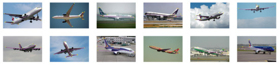
Figure 14.
Qualitative results for the proposed method on ObjectNet3D dataset. The yellow points are the keypoints and the purple segments are the structures.
5.3.3. Performance on the LineMOD Dataset
Different from other literature, we selected just five sequences to evaluate our algorithm which are bench vise, cat, lamp, can, and driller. As discussed in Section 3, we manually select keypoints and structures for these five objects. For bench vise, we select eight keypoints and 5 structures that have rich geometric information, and the pose can be estimated by the combination of these intermediate representations. Similar to the bench vise, we select seven keypoints and four structures for the can, 10 keypoints and six structures for the cat, 11 keypoints and four structures for the driller, and nine keypoints and eight structures for the lamp. For other objects, their structures are not obvious and our algorithm is not suitable for them. The definition of keypoints and structures are shown in Figure 15.
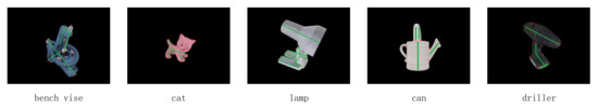
Figure 15.
Keypoints and structures definition of bench vise, cat, lamp, can, and driller. The red points represent the selected keypoints, and the green line segments represent the selected structures.
In Table 7, we compare our method with the state-of-the-art methods in terms of the 2D reprojection metric. A pose is considered correct if the average of the distances is less than 5 pixels. Both our method and SOTA methods use keypoints as intermediate representations to estimate the 6D pose. Bb8 and YOLO-6D use detection frameworks to predict the corners of the 3D bounding box, while PVNET localizes the keypoints by regressing pixel-wise unit vectors and our method jointly estimates the keypoints and structures. On average, our approach is better than Bb8 by 10.12%, YOLO-6D by 8.24%. Compared with PVNET, our method is only 1.5% worse and wins in the driller class.
Table 7.
Comparison with the state-of-the-art methods in terms of the 2D reprojection metric on LineMOD dataset. Bold number indicates the best results.
In Table 8, we compare our method with the state-of-the-art methods in terms of the ADD metric. A pose is considered correct if the average of the distances is less than 10% of the model’s diameter. We first compare with methods in which no refinement is used. DPOD [52] by predicting the dense multi-class 2D-3D correspondence maps. Our method outperforms YOLO-6D, Zhao, and DPOD by a significant margin on the majority of the objects, and only slightly worse than PVNET. Compared with methods in which pose refinement is used, our method also shows competitive results. Similar to our method, HybridPose also combines multiple intermediate representations which are keypoints, edges, and symmetry correspondences. In HybridPose, edge vectors are defined as vectors connecting each pair of keypoints, while in PCK, the structures and keypoints are independent and unrelated. This is the main difference between our method and HybridPose. In addition, in the experiment, HybridPose uses eight keypoints and 28 edges to estimate 6D pose which is much greater than the number of intermediate representations in our method. Considering that our method achieves similar results with HybridPose without using pose refinement, and wins on lamp class, we believe that the structure can better express the geometric information in the input image than the edge. Qualitative results on LineMOD dataset are shown in Figure 16.
Table 8.
Comparison with the state-of-the-art methods in terms of the ADD reprojection metric on LineMOD dataset. Bold number indicates the best results.
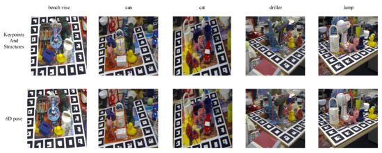
Figure 16.
Qualitative results for the proposed method on LineMOD dataset. The yellow points are the keypoints and the purple segments are the structures.
5.4. Discussion
We conduct discussion on Keypoints Designation, Network Architecture Comparison, and Joint Keypoints and Structures Estimation. All the experiments are conducted on the APE dataset.
5.4.1. Keypoints Designation
We first analyze the keypoints selection schemes used in YOLO-6D and in our methods. As shown in Table 9, we compare the results based on different keypoints set. In ‘SH-Bbox’, we use the eight corners of the 3D bounding box and the center of the aircraft as the keypoints, while in ‘SH-9Kp’, we use nine points selected from the surface as keypoints which are the apex of the aircraft nose, the tips of the left and right wings, the uppermost vertex of the vertical tail, the bottom vertex of the belly, the backmost vertex of the tail and the center of the aircraft. The 3D bounding box can be easily estimated with these nine keypoints. In addition, whether in ‘SH-Bbox’ or ‘SH-9Kp’, we predict the keypoints by the proposed CNN architecture. On average, ‘SH-9Kp’ outperforms ‘SH-Bbox’ by 1.4%. As a result that these two methods differ only in the position of keypoints, selecting keypoints as we discussed in Section 3 results in better performance.
Table 9.
Discussion on APE dataset. Bold number indicates the best result.
Then we conduct a quantitative experiment to show the relationship between the pose estimation accuracy and the number of keypoints. As shown in Figure 17, it is obvious that with the increase of the keypoints’ number the accuracy of pose estimation improves. However, when the number increase from 17 to 23, the accuracy barely improved which indicates that these 17 keypoints have fully represented the aircraft geometry. The reason why we only choose 23 keypoints at most is that it is hard to select other points on the aircraft surface which have as much rich geometric information as these points. If we select some points with rich texture information, the algorithm may fail when over exposure as we discussed in Section 3. These selected 23 points are the apex of the aircraft nose, the leftmost and the rightmost points of the flight compartment windows, the vertexes of the two wings, the vertexes of two horizontal tails, the vertexes of the vertical tail, the backmost vertex of the tail, and the center of the aircraft. What is more, it is impossible to select a continuous number of keypoints because of the aircraft geometry. For example, it is hard to add a point to the keypoints on the basis of ‘SH-9Kp’ because of the symmetry of the aircraft.
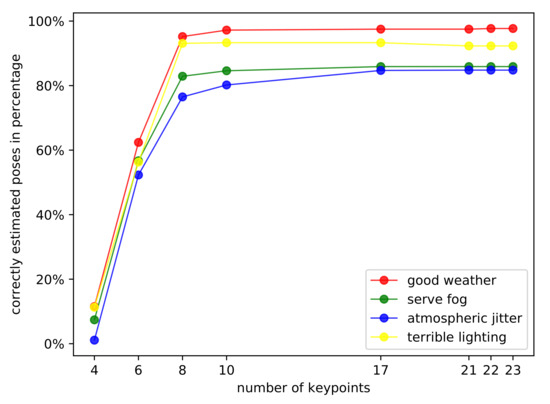
Figure 17.
Discussion on different keypoints numbers for pose estimation on the APE dataset. These results are accuracies in terms of the 2D reprojection metric. With the increase of the keypoints’ number the accuracy of pose estimation improves.
5.4.2. Network Architecture Comparison
As shown in Table 9, we compare our network architecture with YOLO-6D. The ‘SH-Bbox’ and ‘YOLO-6D’ represent the results of our network architecture and YOLO-6D, respectively and they both use the eight corners of the 3D bounding box and the center of the aircraft as keypoints. It is obvious that our network architecture works better in the task of aircraft pose estimation.
The most critical design element of our network is the stacked architecture which allows the network to implicitly learn the topological relationship between the keypoints and structures in a way similar to the attention mechanism. In addition, the combination of bottom-up and top-down processing in the hourglass element makes the network locate the keypoints and structures by the consolidation of features across different scales. The application of intermediate supervision at the end of each model can provide a richer gradient signal to the network and guide the learning procedure to a better optimum. These advantages make our network architecture work better than YOLO which is used in YOLO-6D.
5.4.3. Joint Keypoints and Structures Estimation
As shown in Table 9, we explore the influence of the structures on pose estimation through three experiments. The SH-17Kp+Str’ represents the result of estimating pose by keypoints and structures. Compared with the ‘SH-17Kp’ which just uses keypoints, the combination of keypoints and structures outperforms by 2.5% on average, and when the weather is bad, it works much better especially in the condition of atmospheric jitter which confirms the robustness of structures. To eliminate the effect of the number of intermediate representations, we compare ‘SH-17Kp+Str’ with ‘SH-23Kp’ which have the same number of intermediate variables and find that what can improve the performance of pose estimation is the structures not the number of features.
It can be inferred that, compared with the keypoints, the methods based on multi-feature fusion can get better results in the task of 6D pose estimation because of the robustness of different kinds of geometry features. In the following research, we will adapt more geometric features such as contour to the task of 6D pose estimation.
6. Conclusions
In this article we study the pose estimation of aircraft targets and propose a new approach for this task, called PEKS. First, we leverage multiple intermediate representations to express the geometric information of the target. Keypoints encode the local geometric information and structures encode the geometric relationship between different parts of the object globally. Next, we also propose a PnPS algorithm to recover the 6D pose parameters by keypoints and structures. Experiments show that our method gains a superior performance than the previous keypoints based methods and can estimate the 6D pose accurately in complex weather scenes. What is more, we also introduce a dataset for aircraft pose estimation which is quite challenging because of the complex weather scenes. In the future, we would like to adopt more geometric features to our model and extend our approach to other aircrafts, such as UVA.
Author Contributions
Conceptualization, R.F., Z.W. and T.-B.X.; methodology, R.F.; software, R.F.; validation, R.F., T.-B.X., and Z.W.; formal analysis, R.F.; investigation, R.F.; resources, R.F.; data curation, R.F.; writing—original draft preparation, R.F.; writing—review and editing, T.-B.X.; visualization, R.F.; supervision, Z.W.; project administration, Z.W.; funding acquisition, Z.W. All authors have read and agreed to the published version of the manuscript
Funding
This article was funded by “the National Science Fund for Distinguished Young Scholars of China“ under Grant No. 51625501 and “Aeronautical Science Foundation of China“ under Grant No. 201946051002.
Institutional Review Board Statement
Not applicable.
Informed Consent Statement
Not applicable.
Acknowledgments
This article is supported by the Key Laboratory of Precision Opto-mechatronics Technology, Ministry of Education, Beihang University, China.
Conflicts of Interest
The authors declare no conflict of interest.
References
- Lowe, D.G. Object recognition from local scale-invariant features. In Proceedings of the Seventh IEEE International Conference on Computer Vision, Kerkyra, Greece, 20–27 September 1999; Volume 2, pp. 1150–1157. [Google Scholar]
- Lepetit, V.; Fua, P. Monocular Model-Based 3D Tracking of Rigid Objects: A Survey. Found. Trends Comput. Graph. Vis. 2005, 1, 1–89. [Google Scholar] [CrossRef]
- Collet, A.; Martinez, M.; Srinivasa, S.S. The MOPED framework: Object recognition and pose estimation for manipulation. Int. J. Robot. Res. 2011, 30, 1284–1306. [Google Scholar] [CrossRef]
- Liu, M.Y.; Tuzel, O.; Veeraraghavan, A.; Chellappa, R. Fast directional chamfer matching. In Proceedings of the Seventh IEEE International Conference on Computer Vision, San Francisco, CA, USA, 13–18 June 2010; pp. 1696–1703. [Google Scholar]
- Jurie, F.; Dhome, M. Real Time 3D Template Matching. In Proceedings of the IEEE Computer Society Conference on Computer Vision and Pattern Recognition (CVPR), Kauai, HI, USA, 8–14 December 2001; Volume 1, pp. 1693–1703. [Google Scholar]
- Gu, C.; Ren, X. Discriminative Mixture-of-Templates for Viewpoint Classification. In Proceedings of the European Conference on Computer Vision (ECCV), Crete, Greece, 5–11 September 2020; pp. 408–421. [Google Scholar]
- Zhu, M.; Derpanis, K.G.; Yang, Y.; Brahmbhatt, S.; Zhang, M.; Phillips, C.; Lecce, M.; Daniilidis, K. Single image 3D object detection and pose estimation for grasping. In Proceedings of the 2014 IEEE International Conference on Robotics and Automation (ICRA), Hong Kong, China, 31 May–7 June 2014. [Google Scholar]
- Hinterstoisser, S.; Cagniart, C.; Ilic, S.; Sturm, P.; Navab, N.; Fua, P.; Lepetit, V. Gradient Response Maps for Real-Time Detection of Textureless Objects. IEEE Trans. Pattern Anal. Mach. Intell. 2012, 34, 876–888. [Google Scholar] [CrossRef] [PubMed]
- Su, H.; Qi, C.R.; Li, Y.; Guibas, L.J. Render for CNN: Viewpoint Estimation in Images Using CNNs Trained with Rendered 3D Model Views. In Proceedings of the 2015 IEEE International Conference on Computer Vision (ICCV), Santiago, Chile, 7–13 December 2015; pp. 2686–2694. [Google Scholar] [CrossRef]
- Xiang, Y.; Schmidt, T.; Narayanan, V.; Fox, D. PoseCNN: A Convolutional Neural Network for 6D Object Pose Estimation in Cluttered Scenes. In Proceedings of the Robotics: Science and Systems, Pittsburgh, PA, USA, 26–30 June 2018. [Google Scholar] [CrossRef]
- Massa, F.; Marlet, R.; Aubry, M. Crafting a multi-task CNN for viewpoint estimation. In Proceedings of the British Machine Vision Conference 2016, BMVC 2016, York, UK, 19–22 September 2016; Wilson, R.C., Hancock, E.R., Smith, W.A.P., Eds.; BMVA Press: Norfolk, UK, 2016. [Google Scholar]
- Li, Y.; Wang, G.; Ji, X.; Xiang, Y.; Fox, D. DeepIM: Deep Iterative Matching for 6D Pose Estimation. Int. J. Comput. Vis. 2020, 128, 657–678. [Google Scholar] [CrossRef]
- Wang, G.; Manhardt, F.; Shao, J.; Ji, X.; Navab, N.; Tombari, F. Self6D: Self-Supervised Monocular 6D Object Pose Estimation. In Proceedings of the European Conference on Computer Vision, Glasgow, UK, 23–28 August 2020; pp. 108–125. [Google Scholar]
- Hu, Y.; Fua, P.; Wang, W.; Salzmann, M. Single-Stage 6D Object Pose Estimation. In Proceedings of the 2020 IEEE/CVF Conference on Computer Vision and Pattern Recognition (CVPR), Seattle, WA, USA, 14–19 June 2020; pp. 2930–2939. [Google Scholar]
- Pitteri, G.; Bugeau, A.; Ilic, S.; Lepetit, V. 3D Object Detection and Pose Estimation of Unseen Objects in Color Images with Local Surface Embeddings. In Proceedings of the Asian Conference on Computer Vision, Perth, Australia, Kyoto, Japan, 30 November–4 December 2020. [Google Scholar]
- Busam, B.; Jung, H.J.; Navab, N. I Like to Move It: 6D Pose Estimation as an Action Decision Process. arXiv 2020, arXiv:2009.12678. [Google Scholar]
- Poirson, P.; Ammirato, P.; Fu, C.Y.; Liu, W.; Berg, A.C. Fast Single Shot Detection and Pose Estimation. In Proceedings of the 2016 Fourth International Conference on 3D Vision (3DV), Stanford, CA, USA, 25–28 October 2016. [Google Scholar]
- Michel, F.; Kirillov, A.; Brachmann, E.; Krull, A.; Gumhold, S.; Savchynskyy, B.; Rother, C. Global Hypothesis Generation for 6D Object Pose Estimation. In Proceedings of the IEEE Conference on Computer Vision and Pattern Recognition (CVPR) 2017, Honolulu, HI, USA, 21–26 July 2017. [Google Scholar]
- Kehl, W.; Manhardt, F.; Tombari, F.; Ilic, S.; Navab, N. SSD-6D: Making RGB-Based 3D Detection and 6D Pose Estimation Great Again. In Proceedings of the 2017 IEEE International Conference on Computer Vision (ICCV), Venice, Italy, 22–29 October 2017; pp. 1530–1538. [Google Scholar] [CrossRef]
- Tekin, B.; Sinha, S.N.; Fua, P. Real-Time Seamless Single Shot 6D Object Pose Prediction. In Proceedings of the 2018 IEEE/CVF Conference on Computer Vision and Pattern Recognition, Salt Lake City, UT, USA, 18–23 June 2018; pp. 292–301. [Google Scholar] [CrossRef]
- Peng, S.; Liu, Y.; Huang, Q.; Zhou, X.; Bao, H. PVNet: Pixel-Wise Voting Network for 6DoF Pose Estimation. In Proceedings of the 2019 IEEE/CVF Conference on Computer Vision and Pattern Recognition (CVPR), Long Beach, CA, USA, 16–20 June 2019; pp. 4556–4565. [Google Scholar] [CrossRef]
- Tremblay, J.; To, T.; Sundaralingam, B.; Xiang, Y.; Fox, D.; Birchfield, S. Deep Object Pose Estimation for Semantic Robotic Grasping of Household Objects. In Proceedings of the 2nd Annual Conference on Robot Learning, CoRL 2018, Zürich, Switzerland, 29–31 October 2018; Volume 87, pp. 306–316. [Google Scholar]
- Pavlakos, G.; Zhou, X.; Chan, A.; Derpanis, K.G.; Daniilidis, K. 6-DoF object pose from semantic keypoints. In Proceedings of the 2017 IEEE International Conference on Robotics and Automation (ICRA), Marina Bay Sands, Singapore, 29 May–3 June 2017; pp. 2011–2018. [Google Scholar] [CrossRef]
- Brachmann, E.; Michel, F.; Krull, A.; Yang, M.Y.; Gumhold, S.; Rother, C. Uncertainty-Driven 6D Pose Estimation of Objects and Scenes from a Single RGB Image. In Proceedings of the 2016 IEEE Conference on Computer Vision and Pattern Recognition (CVPR), Las Vegas, NV, USA, 27–30 June 2016; pp. 3364–3372. [Google Scholar] [CrossRef]
- Rad, M.; Lepetit, V. BB8: A Scalable, Accurate, Robust to Partial Occlusion Method for Predicting the 3D Poses of Challenging Objects without Using Depth. In Proceedings of the 2017 IEEE International Conference on Computer Vision (ICCV), Venice, Italy, 22–29 October 2017; pp. 3848–3856. [Google Scholar] [CrossRef]
- Hodan, T.; Barath, D.; Matas, J. EPOS: Estimating 6D Pose of Objects With Symmetries. In Proceedings of the 2020 IEEE/CVF Conference on Computer Vision and Pattern Recognition (CVPR), Seattle, WA, USA, 14–19 June 2020; pp. 11703–11712. [Google Scholar]
- He, Y.; Sun, W.; Huang, H.; Liu, J.; Fan, H.; Sun, J. PVN3D: A Deep Point-Wise 3D Keypoints Voting Network for 6DoF Pose Estimation. In Proceedings of the 2020 IEEE/CVF Conference on Computer Vision and Pattern Recognition (CVPR), Seattle, WA, USA, 14–19 June 2020; pp. 11632–11641. [Google Scholar]
- Chen, X.; Dong, Z.; Song, J.; Geiger, A.; Hilliges, O. Category Level Object Pose Estimation via Neural Analysis-by-Synthesis. In Proceedings of the European Conference on Computer Vision (ECCV), Glasgow, UK, 23–28 August 2020; Volume 26, pp. 139–156. [Google Scholar]
- Manhardt, F.; Wang, G.; Busam, B.; Nickel, M.; Meier, S.; Minciullo, L.; Ji, X.; Navab, N. CPS++: Improving Class-level 6D Pose and Shape Estimation From Monocular Images With Self-Supervised Learning. arXiv 2020, arXiv:2003.05848. [Google Scholar]
- Song, C.; Song, J.; Huang, Q. HybridPose: 6D Object Pose Estimation Under Hybrid Representations. In Proceedings of the 2020 IEEE/CVF Conference on Computer Vision and Pattern Recognition (CVPR), Seattle, WA, USA, 13–19 June 2020; pp. 431–440. [Google Scholar]
- Lepetit, V.; Moreno-Noguer, F.; Fua, P. EPnP: An Accurate O(n) Solution to the PnP Problem. Int. J. Comput. Vis. 2009, 81, 155–166. [Google Scholar] [CrossRef]
- Zheng, Y.; Kuang, Y.; Sugimoto, S.; Strm, K.; Okutomi, M. Revisiting the PnP Problem: A Fast, General and Optimal Solution. In Proceedings of the 2013 IEEE International Conference on Computer Vision, Sydney, Australia, 3–6 December 2013; pp. 2344–2351. [Google Scholar]
- Abdel-Aziz, Y.; Karara, H. Direct Linear Transformation from Comparator Coordinates into Object Space Coordinates in Close-Range Photogrammetry. Photogramm. Eng. Remote Sens. 2015, 81, 103–107. [Google Scholar] [CrossRef]
- Zhang, H.; Li, B.; Zhang, J.; Xu, F. Aerial Image Series Quality Assessment. IOP Conf. Ser. Earth Environ. Sci. 2014, 17, 012183. [Google Scholar] [CrossRef]
- Bay, H. SURF: Speeded Up Robust Features. Comput. Vis. Image Underst. 2006, 110, 404–417. [Google Scholar]
- Rublee, E.; Rabaud, V.; Konolige, K.; Bradski, G. ORB: An efficient alternative to SIFT or SURF. In Proceedings of the 2011 International Conference on Computer Vision, Barcelona, Spain, 6–13 November 2011; pp. 2564–2571. [Google Scholar]
- Kendall, A.; Grimes, M.; Cipolla, R. PoseNet: A Convolutional Network for Real-Time 6-DOF Camera Relocalization. In Proceedings of the 2015 IEEE International Conference on Computer Vision (ICCV), Santiago, Chile, 7–13 December 2015; pp. 2938–2946. [Google Scholar] [CrossRef]
- Scovanner, P.; Ali, S.; Shah, M. A 3-Dimensional SIFT Descriptor and its Application to Action Recognition. Acm Int. Conf. Multimed. 2007, 357. [Google Scholar]
- Bloesch, M.; Czarnowski, J.; Clark, R.; Leutenegger, S.; Davison, A.J. CodeSLAM— Learning a Compact, Optimisable Representation for Dense Visual SLAM. In Proceedings of the 2018 IEEE/CVF Conference on Computer Vision and Pattern Recognition, Salt Lake City, UT, USA, 18–23 June 2018; pp. 2560–2568. [Google Scholar]
- Hsiao, M.; Westman, E.; Zhang, G.; Kaess, M. Keyframe-based dense planar SLAM. In Proceedings of the 2017 IEEE International Conference on Robotics and Automation (ICRA), Marina Bay Sands, Singapore, 29 May–3 June 2017; pp. 5110–5117. [Google Scholar]
- Proenca, P.F.; Gao, Y. Probabilistic RGB-D Odometry based on Points, Lines and Planes Under Depth Uncertainty. Robot. Auton. Syst. 2017, 104, 25–39. [Google Scholar] [CrossRef]
- Newell, A.; Yang, K.; Deng, J. Stacked Hourglass Networks for Human Pose Estimation. In Proceedings of the European Conference on Computer Vision, Amsterdam, The Netherlands, 8–16 October 2016; pp. 483–499. [Google Scholar]
- Busto, P.P.; Gall, J. Joint Viewpoint and Keypoint Estimation with Real and Synthetic Data. In Proceedings of the German Conference on Pattern Recognition, Stuttgart, Germany, 9–12 October 2019; pp. 107–121. [Google Scholar]
- Wei, S.; Ramakrishna, V.; Kanade, T.; Sheikh, Y. Convolutional Pose Machines. In Proceedings of the 2016 IEEE Conference on Computer Vision and Pattern Recognition (CVPR), Las Vegas, NV, USA, 27–30 June 2016; pp. 4724–4732. [Google Scholar] [CrossRef]
- Mousavian, A.; Anguelov, D.; Flynn, J.; Kosecka, J. 3D Bounding Box Estimation Using Deep Learning and Geometry. In Proceedings of the 2017 IEEE Conference on Computer Vision and Pattern Recognition, CVPR 2017, Honolulu, HI, USA, 21–26 July 2017; pp. 5632–5640. [Google Scholar] [CrossRef]
- Teng, X.; Yu, Q.; Luo, J.; Zhang, X.; Wang, G. Pose Estimation for Straight Wing Aircraft Based on Consistent Line Clustering and Planes Intersection. Sensors 2019, 19, 342. [Google Scholar] [CrossRef] [PubMed]
- Vakhitov, A.; Funke, J.; Moreno-Noguer, F. Accurate and Linear Time Pose Estimation from Points and Lines. In Proceedings of the Computer Vision—ECCV 2016—14th European Conference, Amsterdam, The Netherlands, 11–14 October 2016; Proceedings, Part VII. Leibe, B., Matas, J., Sebe, N., Welling, M., Eds.; Springer: Berlin/Heidelberg, Germany, 2016; Volume 9911, pp. 583–599. [Google Scholar] [CrossRef]
- Geiger, A.; Lenz, P.; Stiller, C.; Urtasun, R. Vision meets robotics: The KITTI dataset. Int. J. Robot. Res. 2013, 32, 1231–1237. [Google Scholar] [CrossRef]
- Xiang, Y.; Kim, W.; Chen, W.; Ji, J.; Choy, C.B.; Su, H.; Mottaghi, R.; Guibas, L.J.; Savarese, S. ObjectNet3D: A Large Scale Database for 3D Object Recognition. In Proceedings of the Computer Vision—ECCV 2016—14th European Conference; Proceedings, Part VIII. Leibe, B., Matas, J., Sebe, N., Welling, M., Eds.; Springer: Berlin/Heidelberg, Germany, 2016; Volume 9912, pp. 160–176. [Google Scholar] [CrossRef]
- Hinterstoisser, S.; Lepetit, V.; Ilic, S.; Holzer, S.; Navab, N. Model Based Training, Detection and Pose Estimation of Texture-Less 3D Objects in Heavily Cluttered Scenes. In Proceedings of the Asian Conference on Computer Vision, Daejeon, Korea, 5–9 November 2012. [Google Scholar]
- Tulsiani, S.; Malik, J. Viewpoints and keypoints. In Proceedings of the 2015 IEEE Conference on Computer Vision and Pattern Recognition (CVPR), Boston, MA, USA, 7–12 June 2015; pp. 1510–1519. [Google Scholar] [CrossRef]
- Zakharov, S.; Shugurov, I.; Ilic, S. DPOD: 6D Pose Object Detector and Refiner. In Proceedings of the 2019 IEEE/CVF International Conference on Computer Vision (ICCV), Seoul, Korea, 27–28 October 2019; pp. 1941–1950. [Google Scholar] [CrossRef]
- Li, Z.; Wang, G.; Ji, X. CDPN: Coordinates-Based Disentangled Pose Network for Real-Time RGB-Based 6-DoF Object Pose Estimation. In Proceedings of the 2019 IEEE/CVF International Conference on Computer Vision (ICCV), Seoul, Korea, 27–28 October 2019; pp. 7677–7686. [Google Scholar] [CrossRef]


Publisher’s Note: MDPI stays neutral with regard to jurisdictional claims in published maps and institutional affiliations. |
© 2021 by the authors. Licensee MDPI, Basel, Switzerland. This article is an open access article distributed under the terms and conditions of the Creative Commons Attribution (CC BY) license (http://creativecommons.org/licenses/by/4.0/).