The Analysis and Modelling of the Quality of Information Acquired from Weather Station Sensors

Abstract

This article explores the quality of information acquired from weather station sensors. A review of literature in this field concludes that most publications concern the analysis of data acquired from weather station sensors and their characteristic properties, estimating the missing values from the data, and assessing the quality of weather information. Despite the large collection of studies devoted to these issues, there is no comprehensive approach that would consider the modelling of information uncertainty. Therefore, the article presents a proprietary method of analysing and modelling the uncertainty of the weather station sensors’ information quality. For this purpose, the structure of a real meteorological station and the measurement data obtained from it were analysed. Next, an information quality model was developed using the certainty factor (CF) of hypothesis calculation. The developed method was verified on an exemplary real meteorological station. It was found that this method enables the improvement of the quality of information obtained and processed in a multi-sensor system. This becomes practical when the influence of individual measurement system elements on the information quality reaching the recipient is determined. An example is furnished by a demonstration of the usage of two sensors to improve the information quality.

1. Introduction

Information collected from weather station sensors is currently employed in many economy fields, e.g., agriculture, transport [1], and tourism. Based on the received information, it is possible to take rational actions to implement the specific activity in particular areas. This applies particularly to systems classified as critical national infrastructure. Many publications describe and analyse the acquired sensor data and their characteristic properties and estimate missing data in the original meteorological information. Some studies also present research on the quality of information obtained from these sensors. However, no approach takes into account uncertainty estimation of the information quality. When applied to the process of estimating the quality of information obtained from meteorological station sensors, uncertainty modelling allows one to increase the forecasted data reliability.

Analysing the state of knowledge in the field discussed in this article but also delving into the achievements of the scientific community, the following areas can be distinguished:

• publications describing meteorological stations, applied sensors, and construction solutions [1,2,3,4],
• publications on analyses of data obtained from sensors and their correctness,
• publications on the quality of information obtained from sensors used in meteorological stations,
• publications on the estimation of missing data in meteorological information,
• publications on the quality assessment of weather information.

The listed main research areas directly related to the subject of this article are analysed in detail below.

The study described in [5] describes issues related to the adoption of wireless sensor networks to assess air quality. The authors have rightly noticed that, having data from individual sensors on temperature, humidity, carbon monoxide (CO), and carbon dioxide (CO₂), it is possible to estimate air quality and decide about the occurrence of an emergency in the warning system. For this purpose, they implemented the classification tree algorithm with regard to entropy and information enhancement. This approach has a practical application, but it does not consider some factors influencing the quality of the information received from individual sensors.

Additionally, in the area of transport (especially in autonomous vehicles and on motorways), the quality of information obtained from meteorological sensors is crucial [6]. Study in this area is presented in monograph [7]. Owing to this, it is possible to detect dangerous weather events and inform drivers about them immediately. Similar studies of stationary weather stations applied in intelligent transport systems (ITS) are presented in [8].

A similar approach in the analysis of the obtained data from meteorological stations was adopted by the authors in the study [9]. They applied decision tree algorithms, analysing precipitation and minimum and maximum temperatures separately. Thanks to the application of algorithms devised by the authors, it is possible to identify flawed sequences contained in meteorological sensors. Similar studies regarding air quality classification using specific algorithms and a decision tree are presented in publication [5]. Inquiry in this area concerns not only land meteorological stations but also marine ones [10].

It is likely to estimate the correctness of meteorological data by comparing them with data from neighbouring meteorological stations. Then, it is possible to determine the consistency of data relating to a given meteorological phenomenon in a specific area [11].

The study described in [12] presents studies aimed at determining the forecast using a hybrid computing network. This approach enables forecasting weather conditions with an insufficient number of meteorological stations.

The next research area, highlighted by the authors of this article, contains publications on the estimation of missing data in meteorological information. Scientifically interesting considerations are presented in the study [13]. It proposes to employ a method consisting in finding time intervals with similar rainfall patterns. Thanks to their analysis, it is possible to interpolate the missing data with better quality compared to the methods used so far.

A study [14] also describes work in this research area. The team of authors proposed models enabling temperature interpolation in a geographical system for agricultural purposes. The conducted analyses resulted in finding that the application of multi-line regression is most beneficial.

Authors adopt various approaches to assess the quality of weather information. One of them is the quality of the data stored in big data. As data from many weather stations equipped with many different sensors are most often (except in sparsely populated areas) available, it is possible to pre-process them in order to eliminate errors. This approach was presented in publication [15]. By pre-processing the data, a weather forecasting system that used data of better quality could be designed.

In order to improve the quality of weather information, a data fusion solution is also employed. In this way, it is possible to combine data from different sensors. This increases the reliability of the weather information. This approach was described in the article [16]. The authors analysed the applied solutions in the area of intelligent transport systems. They considered that, in the fusion of data from sensors, the most important is the application of: fuzzy technique, ranging technique, integrated technique, and clustering technique. Despite considering these techniques and analysing their advantages, these lack the possibility to model uncertainty in estimating information quality. Similar considerations in this area in the field of transport are presented in the study [17]. This is a very important issue in the aspect of current research and design of autonomous vehicles. It also seems essential to use modelling of the uncertainty of estimating information quality, because it is possible to increase the level of safety of the means of transport.

Methods of variational assimilation of measurement data from various observational systems, including imagery, can also be distinguished among scientific studies in weather information analysis. In publication [18], the authors proposed using a proprietary data assimilation algorithm, which they presented in detail in a mathematical notation. However, they did not take into account the information quality from individual sources.

Some scientific studies propose the use of neural networks for the analysis of weather information [19]. The study in article [20] posits the application of deep neural networks (DNN) with the object of estimating the amount of precipitation on the basis of radar, microwave, and infrared data. The conducted simulations confirm the validity of using DNN to improve the forecast of the amount of precipitation. However, it seems that, by applying uncertainty modelling of estimating information quality, it is possible to increase the accuracy of the forecasted data. Therefore, the authors of this article conducted scientific scrutiny in this direction.

The investigation of the status of the issue allows one to conclude that most of the studies concern the analysis of the correctness of the obtained data from sensors and weather forecasting with the application of various algorithms. To the best of our knowledge, no publications considered the quality of the information received from a meteorological station at the time of conducting the studies. Studies in this area together with the results are presented by the authors in this article.

2. Uncertainty Modelling Applied to Estimate the Quality of Information Obtained from Sensors of a Meteorological Station

The information quality estimation method uses the calculations of the certainty factor of the hypothesis. The applied CF modelling is based on dependent and independent connections. Such modelling makes it possible to estimate the impact of selected quality dimensions and their factors on the quality of information and to identify reliable measurements from several different data sources (e.g., data from different types of sensors).

2.1. Information Quality

There are many ways to describe information quality [21,22,23]. The best known are the descriptions in reports and publications related to Massachusetts Institute of Technology Information Quality Program (MITIQ) [24]. They developed, among other things, an information quality model based on sixteen dimensions. Ultimately, the MITIQ defined the dimensions of information quality, which are described as [24,25,26,27]:

• Availability (D_av)—a dimension that defines the possibility of using an information and communication technologies (ICT) element on demand, at a given time, and by an authorized process. This dimension is directly related to information security.
• Appropriate amount of data (D_aad)—a dimension that determines how much data are adequate to complete the task while indicating that the amount is sufficient and more data could reduce information quality.
• Believability (D_bel)—a dimension which determines the degree to which information reflects reality. It may also be related to the credibility of the information source itself.
• Completeness (D_com)—a dimension that determines whether the data are sufficient to perform a specific task.
• Concise representation (D_ccr)—a dimension that determines the degree to which data are represented.
• Consistent representation (D_csr)—a dimension that specifies to what extent data are represented in the same format.
• Ease of manipulation (D_eom)—a dimension that determines how easily these data can be processed when applied to other tasks.
• Free of error (D_foe)—the dimension that determines the extent to which the data are error-free.
• Interpretability (D_inter)—a dimension that defines the extent to which data are clear and represented in appropriate languages and symbols.
• Objectivity (D_obj)—the dimension which determines to what extent data are not subjective.
• Relevancy (D_relev)—a dimension that determines the usefulness of data in performing a specific task.
• Reputation (D_reput)—a dimension that determines the extent to which data are assessed in terms of its sources and content.
• Security (D_sec)—a dimension that determines the access limits to data to isolate them from unauthorized access.
• Timeliness (D_tim)—the dimension that determines the extent to which data are available on time to complete a task.
• Understandability (D_uns)—a dimension that determines the understandability of data.
• Value-added (D_vadd)—a dimension that determines the benefits of using data and whether they themselves are beneficial to the task.

Figure 1 shows all the above-mentioned dimensions affecting information quality. Each of the dimensions has a direct impact on information quality. Assuming that each value of the dimension (dimension factor) may vary in the range from 0 to 1, the dimension that does not affect the quality of information has the value of 1. The dimension that significantly reduces the quality has the value of 0. Taking the value range <0.1> allows calculating information quality by statistical methods (e.g., a probability of error Pe can be used as the free of error dimension coefficient = 1—Pe) but also adopting methods of estimating uncertainty, such as mathematical evidence based on the Dempster–Shafer theory or CF modelling [28,29,30].

In general, information quality (IQ) consists of the above-mentioned dimensions. Thus, IQ can be described by the formula:

IQ = f(w₁,w₂,…,w_m),

(1)

where:

• m—the number of dimensions, information quality components (equals 16 according to the number of the above dimensions),
• w—a variable that determines the impact of a given dimension (i.e., a value in the range <0.1>).

In the study below, modelling based on the certainty factor of hypothesis [31,32] was applied.

2.2. Modelling Certainty Factor of Hypothesis

As mentioned above, a convenient model for describing information quality may be modelling based on CF of the hypothesis. It is assumed that this factor’s value is a direct value indicating the information quality related to the given hypothesis.

Accurate presentation requires describing formalisms [31,32]. The formal simplified description of the certainty factor is defined as:

$$\mathrm{CF}\left(\mathrm{s}\right)=\mathrm{MB}\left(\mathrm{s}\right)-\mathrm{MD}\left(\mathrm{s}\right),$$

(2)

where:

• CF—certainty factor,
• MB—knowledge mapping, i.e., measure of belief,
• MD—hypothesis based on some information.

One has to bear in mind that:

$$\mathrm{MB}\stackrel{}{\to }\langle 0,1\rangle ;\mathrm{MD}\stackrel{}{\to }\langle 0,1\rangle ;\mathrm{CF}\in \langle -1,1\rangle ,$$

(3)

Interpretation of the measure of belief (MB) and the measure of disbelief (MD) to probability can be defined as:

$$\mathrm{CF}\left(\mathrm{s}\right)\{\begin{array}{c}1\\ \mathrm{MB}\left(\mathrm{s}\right)\\ \begin{array}{c}0\\ \begin{array}{c}-\mathrm{MD}\left(\mathrm{s}\right)\\ -1\end{array}\end{array}\end{array}\begin{array}{c}\mathrm{P}\left(\mathrm{s}\right)=1\\ \mathrm{P}\left(\mathrm{s}\right)>\mathrm{P}\left(\neg \mathrm{s}\right)\\ \begin{array}{c}\mathrm{P}\left(\mathrm{s}\right)=\mathrm{P}\left(\neg \mathrm{s}\right)\\ \begin{array}{c}\mathrm{P}\left(\mathrm{s}\right)<\mathrm{P}\left(\neg \mathrm{s}\right)\\ \mathrm{P}\left(\mathrm{s}\right)= 0\end{array}\end{array}\end{array},$$

(4)

where:

• P—probability,
• s—hypothesis based on some information.

However, as mentioned, we do not aim at determining probability because our quality measure is to be related to the CF of final hypothesis of the model.

Since there are many varieties of CF modelling, the basic dependents used in this paper are described below [31,32].

2.2.1. Parallel basic model

The formula for calculating the transition according to Figure 2 between two parallel observations and the hypothesis are described as [30]:

$$\mathrm{CF}\left(\mathrm{h},\mathrm{e}1,\mathrm{e}2\right)=\{\begin{array}{ccc}\mathrm{CF}\left(\mathrm{h},\mathrm{e}1\right)+\mathrm{CF}\left(\mathrm{h},\mathrm{e}2\right)-\mathrm{CF}\left(\mathrm{h},\mathrm{e}1\right)\cdot \mathrm{CF}\left(\mathrm{h},\mathrm{e}2\right)& \mathrm{if}& \mathrm{CF}\left(\mathrm{h},\mathrm{e}1\right)\ge 0 \mathrm{and} \mathrm{CF}\left(\mathrm{h},\mathrm{e}2\right)\ge 0\\ \frac{\mathrm{CF}\left(\mathrm{h},\mathrm{e}1\right)+\mathrm{CF}\left(\mathrm{h},\mathrm{e}2\right)}{1-\min (\left|\mathrm{CF}\left(\mathrm{h},\mathrm{e}1\right)\right|;|\mathrm{CF}\left(\mathrm{h},\mathrm{e}2\right)\mid )}& \mathrm{if}& \mathrm{CF}\left(\mathrm{h},\mathrm{e}1\right)\cdot \mathrm{CF}\left(\mathrm{h},\mathrm{e}2\right)<0\\ \mathrm{CF}\left(\mathrm{h},\mathrm{e}1\right)+\mathrm{CF}\left(\mathrm{h},\mathrm{e}2\right)+\mathrm{CF}\left(\mathrm{h},\mathrm{e}1\right)\cdot \mathrm{CF}\left(\mathrm{h},\mathrm{e}2\right)& \mathrm{if}& \mathrm{CF}\left(\mathrm{h},\mathrm{e}1\right)<0 \mathrm{and} \mathrm{CF}\left(\mathrm{h},\mathrm{e}2\right)<0\end{array},$$

(5)

2.2.2. Serial basic model

In the case of a serial model for positive values (such appears in the modelling described later), according to Figure 3, the following dependent was used [31,32]:

$$\mathrm{CF}\left(\mathrm{h},\mathrm{e}1,\mathrm{e}2\right)=\{\begin{array}{ccc}\mathrm{CF}\left(\mathrm{e}2,\mathrm{e}1\right) · \mathrm{CF}\left(\mathrm{h},\mathrm{e}2\right)& \mathrm{if}\hfill & \mathrm{CF}\left(\mathrm{e}2,\mathrm{e}1\right)>0\hfill \\ 0\hfill & \mathrm{if}\hfill & \mathrm{CF}\left(\mathrm{e}2,\mathrm{e}1\right)\underset{\_}{<}0\hfill \end{array},$$

(6)

Both connections, parallel and series, can be reduced to one connection, as shown in Figure 4. This property enables the simplification of calculations in the model proposed in the next chapter.

In the following considerations, the final hypothesis’s certainty factor is the value of the information quality.

2.3. Parallel-Serial Model of the Analysed Solution of the Meteorological Station

In literature, many models are describing various states of information. The most developed ones can be found in [33], where they are called information processes. The following types of these information processes are listed below (Figure 5):

• generating,
• collecting,
• storage,
• processing [34,35,36,37],
• transmitting [38,39],
• sharing,
• interpretation.

In Figure 5, the three information states are combined into one because they usually occur together. Such a presentation of information processes also makes it possible to slightly simplify the model, which does not affect the model’s overall accuracy.

A generalised information quality model can be presented as follows. Each of the previously mentioned information states can be a consecutive node of the information quality model and generally presented in Figure 6 [40].

In the presented case, the information quality model is limited to five information states, of which the fourth state contains three information processes, as shown in Figure 5. The general model consists of five hypotheses related to information states (Figure 6) and contains groups of factors, which influence measurement quality as below:

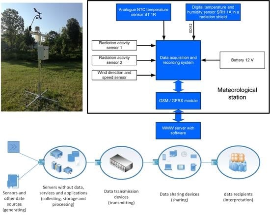
• Dimensions related to the main data source. In this case, the data source is the weather station. The dimensions associated with this source influence the value of the indirect hypothesis h1. In the case of data source redundancy, the h1 hypothesis consists of many indirect hypotheses.
• Dimensions related to collecting, storing, and processing of data. In this case, it is a computer system dedicated to performing specific tasks. The dimensions related to this state of information influence the value of the indirect hypothesis h2.
• Dimensions related to data transmission. This group includes devices for data transport and transmission. Data transport factors influence the value of the indirect hypothesis h3.
• Dimensions related to data sharing systems. This group includes imaging and sound devices transmitting data for interpretation as well as interfaces if the interpreter is a computer system, e.g., artificial intelligence (AI). The dimensions related to this state of information influence the value of the indirect hypothesis h4.
• Dimensions related to data interpretation. This group includes people and—as in this case –computer systems, e.g., AI. The dimensions related to this state of information influence the value of the indirect hypothesis h5.

Each of the above points can be described with a full information quality model presented in Section 2.1. A schematic representation of such a model is shown in Figure 7.

In the case of the qualitative model, only those dimensions that significantly affect the result are of any interest. Thus, in the following description, only those factors that have such an influence are presented.

The final hypothesis is h—the data have been correctly interpreted. It consists of dependent indirect hypotheses (Figure 7):

• h1a—Basic data source provides valid data. Based on the observations of e1a.
• h1b—Auxiliary data source provides valid data. Based on observations from e1b.
• h1—The weather station delivers valid data. Based on observations of e1a and e1b.
• h2—Data collection, storage, and processing work properly. Based on the observations of e2.
• h3—Data transport systems work properly. Based on observations from e3.
• h4—Data sharing systems work properly and share data in the correct way. Based on the observations of e4.
• h5—Data are interpreted correctly. Based on observations e5.

Each of the indirect hypotheses created on the basis of observations results from observing factors in a given group. In order to simplify the final calculations, the following description includes only some of the events and the observations that may affect the quality of information.

The indirect hypothesis based on the observations e1a consists of independent observations:

• e1a.1—The detector is working properly.
• e1a.2—Detector failure.
• e1a.3—Lack of power.

The indirect hypothesis based on the observations e1b consists of independent observations:

• e1b.1—The detector is working properly.
• e1b.2—Detector failure.
• e1b.3—Lack of power.

The indirect hypothesis based on the observations e2 consists of independent observations:

• e2.1—Data collection, storage, and processing work properly.
• e2.2—Interruption of data transmission.
• e2.3—Data are not collected (e.g., lack of resources).
• e2.4—The data are not processed (e.g., insufficient capacity of the data processing system).

The indirect hypothesis based on the observations e3 consists of independent observations:

• e3.1—Data transport systems are working properly.
• e3.2—Link failure.
• e3.3—Power failure of network devices [41,42,43].

The indirect hypothesis based on the observations e4 consists of independent observations:

• e4.1—Data sharing systems are working properly and sharing data in the correct way.
• e4.2—Data transmission interruption [44,45].
• e4.3—Defective data sharing methods.

The indirect hypothesis based on the observations e5 consists of independent observations:

• e5.1—Data are interpreted correctly.
• e5.2—Badly trained staff (e.g., does not understand the message).
• e5.3—Incorrect data response of the interpreter.

Figure 8 shows a graph of the model of indirect hypotheses h1a. The hypotheses models h1b, h3, h4, and h5 are similar.

Figure 9 shows the graph of the model of indirect hypotheses h2.

Figure 10 shows the graph of the model of indirect hypotheses h1.

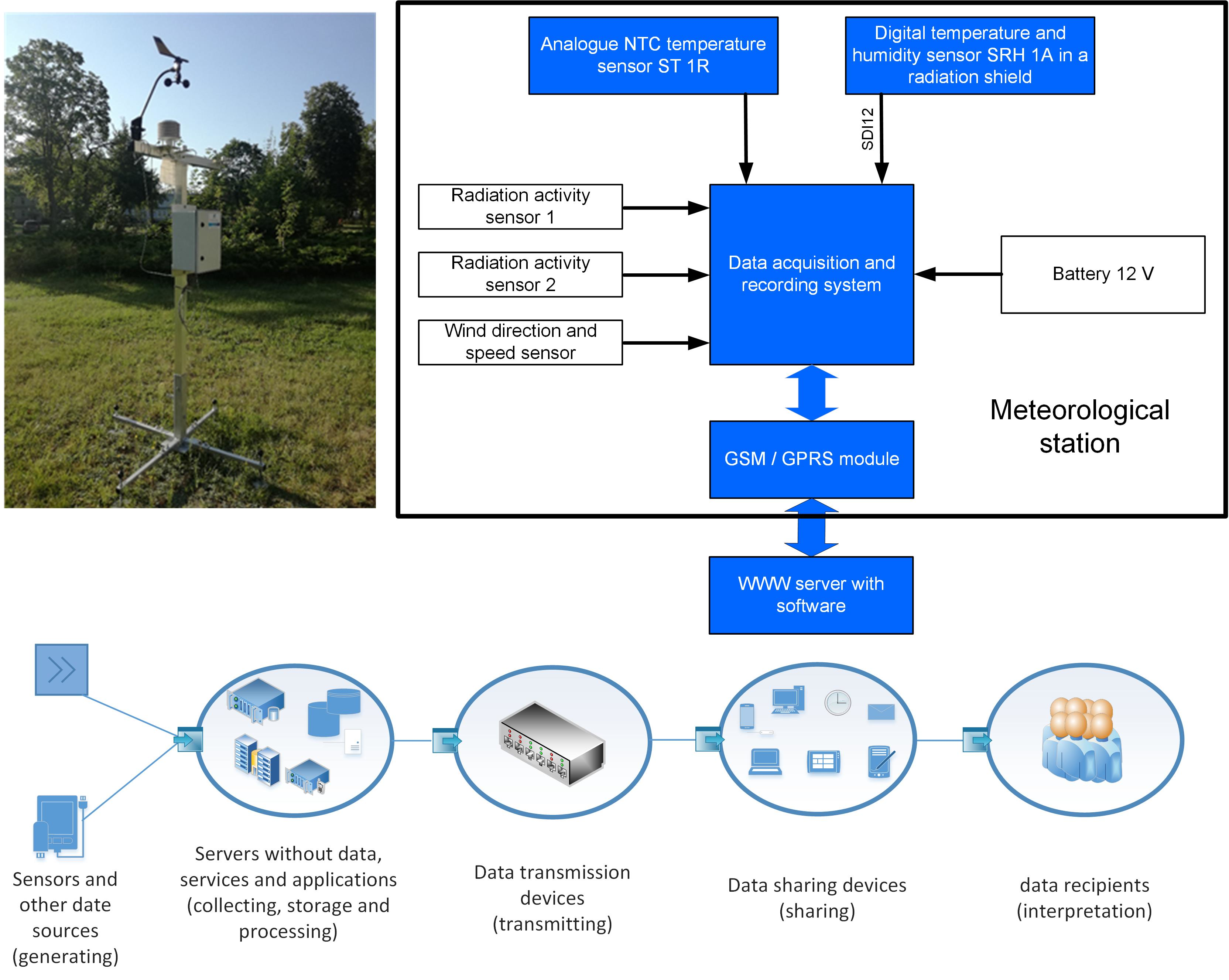
3. Method Verification and its Computer Exemplification

Sample calculations are presented below. Observation coefficients were estimated for the real measuring station shown in Figure 11 (observations e1a, e1b, and e2) and based on the authors’earlier publications [40,46]. The meteorological station is located in Poland in the northwest part of Warsaw on the premises of the Military University of Technology (geographical coordinates: 52°15′10.6″ N and 20°53′58.9″ E). The measurements were taken in May 2020. During the measurements, the following weather parameters were recorded: wind speed from 0 m/s to 12 m/s, temperature range from 3 °C to 25 °C, relative humidity from 35% to 90%.

The meteorological station includes the following sensors:

• Digital temperature and relative humidity sensor marked with the catalogue symbol SRH1A (abbreviation comes from the words: sensor, relative humidity) placed in an anti-radiation shield.
• Analogue temperature sensor with negative temperature coefficient (NTC) thermistor marked with the catalogue symbol ST1R (abbreviation comes from words: sensor, temperature) placed in an anti-radiation shield.
• Wind speed and direction sensor.
• Two independent solar radiation intensity sensors.

Additionally, the station includes a “Micropower” module which records and transmits data to the server. The station is situated on a two-meter-high aluminium mast. The digital temperature and relative humidity sensor marked with the catalogue symbol SRH1A is a measurement device which can operate both in external conditions and inside buildings. Its basic technical data [47] are shown in

Table 1. Technical data of the digital temperature and relative humidity sensor.

Parameter	Relative Humidity (RH) Measurement	Temperature Measurement
Measurement range	0 … 100%RH	−40 … +70 °C
Accuracy at 25 °C	±1.8%RH (0 … 90%RH) ±3.0%RH (>90%RH)	±0.3 °C (0 … 70 °C), ±0.5 °C for the remaining values
Nonlinearity	<0.1%RH	-
Long-term stability	<0.25%RH/year	<0.02 °C/year
Measurement resolution	0.01%RH	0.01 °C

.

Analogue NTC temperature sensor with the catalogue symbol ST1R [48] is meant to measure air temperature. Its case is made of stainless steel which allows the use of the sensor in difficult atmospheric conditions. The basic parameters are as follows:

• Operation temperature range −50 …+70 °C,
• Measurement accuracy ±0.5 °C,
• Measurement element 100 kΩ NTC,
• Sensor’s dimensions ø6 × 60 mm,
• Level of security IP 67.

In the block diagram (Figure 12) of the meteorological station, the metrological data processing path for ambient temperature consists of blocks filled with background.

With reference to the diagram in Figure 5, the individual elements are related to the observations in accordance with the following list:

• e1a—these are observations related to an analogue temperature sensor with a cable connection,
• e1b—these are observations related to a digital temperature sensor with a cable connection,
• e2—these are observations related to the system for data acquisition and recording with an input expansion card and a memory card,
• e3—these are observations related to the digital cellular communication module.

The element related to e1a observations consists of an analogue NTC (negative temperature coefficient) temperature sensor with catalogue symbol ST1R, working properly in the range of 11–16 V supply voltage and a cable connection with a recorder. As described in the previous section of the article, the following characteristic observations were distinguished for this element:

• e1a.1—the sensors work correctly, the observation coefficient is 0.95,
• e1a.2—faulty analogue sensor or broken signal wire, observation coefficient is 0.02 based on observations, data from the manufacturer, and wiring reliability analysis,
• e1a.3—battery voltage supply below 11 V or interrupted power line, the observation coefficient is 0.04 based on observation of the facility exploitation.

The e1b element consists of a digital temperature sensor with catalogue symbol SRH1A that works correctly in the range of supply voltage 4–16 V and an interface for serial data transmission in the serial–digital interface, standard for microprocessor-based sensor (SDI-12 standard). As described in the previous chapter, characteristic observations were distinguished for this element:

• e1b.1—the sensor and the SDI-12 link work correctly, the observation factor is 0.99,
• e1b.2—faulty sensor or serial data transmission error, the observation coefficient is 0.01 determined on the basis of observations and data from the manufacturer,
• e1b.3—battery voltage supply below 4 V or interrupted power line, the observation coefficient is 0.002 based on observation of the facility exploitation.

Element 2 is a specialised recorder based on a single-chip micropower data logger microcontroller, requiring a supply voltage of 5–16 V and made in a technology that meets the IP67 standard of resistance to environmental factors. The recorder additionally includes an SDI-12 standard input expansion module and a memory card. Based on the observations, it was determined that the following events can occur in the e2 element:

• e2.1—the recorder is working correctly, the observation coefficient is 0.99,
• e2.2—faulty microcontroller or expansion modules, the observation factor is 0.005 determined on the basis of observations and data from the manufacturer,
• e2.3—data archiving not possible due to overflow or memory card fault, the observation factor is 0.004 determined on the basis of observations and data from the manufacturer
• e2.4—battery supply voltage below 5 V or power line interruption, the observation factor is 0.002 based on the observation of the facility exploitation.

The values in

Table 2. Observation coefficients (hxx, exx.x).

	e1a	e1b	e2	e3	e4	e5
1.	0.95	0.99	0.99	0.892	0.865	0.781
2.	−0.02	−0.01	−0.005	−0.122	−0.152	−0.185
3.	−0.04	−0.002	−0.004	−0.03	−0.114	−0.251
4.			−0.002

were calculated on the basis of the annual observation time of the meteorological station, which is shown in Figure 11. The states of fitness and unfitness of individual elements included in the tested meteorological station were determined [49,50,51,52].

The value of the maximum coefficient of hypothesis (h1, IQ1max) was assumed at a level close to the value 1, namely 0.9999.

The coefficients of successive indirect hypotheses are determined using Equation (5).

$$\begin{array}{c}\mathrm{CF}\left(\mathrm{h}1\mathrm{a},\mathrm{e}1\mathrm{a}.1,\mathrm{e}1\mathrm{a}.2\right)=\frac{\mathrm{CF}\left(\mathrm{h}1\mathrm{a},\mathrm{e}1\mathrm{a}.1\right)+\mathrm{CF}\left(\mathrm{h}1\mathrm{a},\mathrm{e}1\mathrm{a}.2\right)}{1-\min \left(\left|\mathrm{CF}\left(\mathrm{h}1\mathrm{a},\mathrm{e}1\mathrm{a}.1\right)\right|;\left|\mathrm{CF}\left(\mathrm{h}1\mathrm{a},\mathrm{e}1\mathrm{a}.2\right)\right|\right)}\\ =\frac{0.95+(-0.02)}{1-\min \left(\left|0.95\right|;\left|(-0.02)\right|\right)}=\frac{0.83}{0.88}\widetilde{=}0.94898\end{array},$$

(7)

$$\begin{array}{c}\mathrm{h}1\mathrm{a} = \mathrm{CF}\left(\mathrm{h}1\mathrm{a},\mathrm{e}1\mathrm{a}.1,\mathrm{e}1\mathrm{a}.2,\mathrm{e}1\mathrm{a}3\right)=\frac{\mathrm{CF}\left(\mathrm{h}1\mathrm{a},\mathrm{e}1\mathrm{a}.1,\mathrm{e}1\mathrm{a}.2\right)+\mathrm{CF}\left(\mathrm{h}1\mathrm{a},\mathrm{e}1\mathrm{a}.3\right)}{1-\min \left(\left|\mathrm{CF}\left(\mathrm{h}1\mathrm{a},\mathrm{e}1\mathrm{a}.1,\mathrm{e}1\mathrm{a}.2\right)\right|;\left|\mathrm{CF}\left(\mathrm{h}1\mathrm{a},\mathrm{e}1\mathrm{a}.3\right)\right|\right)}\\ =\frac{0.94898 +(-0.04)}{1-\min \left(\left|0.94898 \right|;\left|(-0.04)\right|\right)}=\frac{0.9927}{0.96}\widetilde{=}0.94685\end{array},$$

(8)

h1b, h2, h3, h4, and h5 are calculated in a similar way and they amount to:

$$\begin{array}{c}\mathrm{h}1\mathrm{b} \widetilde{=}0.98988\\ \begin{array}{c}\mathrm{h}2 \widetilde{=}0.98989\\ \mathrm{h}3 \widetilde{=}0.87319\\ \begin{array}{c}\mathrm{h}4 \widetilde{=}0.82032\\ \mathrm{h}5 \widetilde{=}0.64124\end{array}\end{array}\end{array}$$

The next step is to determine the value of h1. Similarly, using Equation (5), the value of h1 is determined. h1a and h1b are replaced by values h1a′ = −1 + h1a and h1b′ = −1 + h1b.

$$\mathrm{CF}(\mathrm{h}1\mathrm{a}\prime ,\mathrm{IQ}1\max )=\frac{\mathrm{CF}(\mathrm{h}1,\mathrm{IQ}1\max )+\mathrm{CF}(\mathrm{h}1\mathrm{a}\prime ,\mathrm{IQ}1\max )}{1-\min \left(\left|\mathrm{CF}(\mathrm{h}1,\mathrm{IQ}1\max )\right|;\left|\mathrm{CF}(\mathrm{h}1,\mathrm{h}1\mathrm{a}\prime )\right|\right)}=\frac{0.9999 +(-0.05315)}{1-\min (|0.9999|;\left|(-0.05315)\right|)}\widetilde{=}0.999894,$$

(9)

$$\begin{array}{c}\mathrm{h}1 = \mathrm{CF}\left(\mathrm{h}1,\mathrm{h}1\mathrm{a}\prime ,\mathrm{h}2\mathrm{b}\prime ,\mathrm{IQ}1\max \right)=\frac{\mathrm{CF}\left(\mathrm{h}1\mathrm{a}\prime ,\mathrm{IQ}1\max \right)+\mathrm{CF}\left(\mathrm{h}1\mathrm{b}\prime ,\mathrm{IQ}1\max \right)}{1-\min \left(\left|\mathrm{CF}\left(\mathrm{h}1\mathrm{a}\prime ,\mathrm{IQ}1\max \right)\right|;\left|\mathrm{CF}\left(\mathrm{h}1\mathrm{b}\prime ,\mathrm{IQ}1\max \right)\right|\right)}\\ =\frac{0.999894 +(-0.01012)}{1-\min \left(\left|0.999894\right|;\left|(-0.01012)\right|\right)}\widetilde{=}0.999893 \end{array},$$

(10)

Using equation 6, the final hypothesis coefficient can be determined as:

$$\mathrm{h} = \mathrm{h}1 · \mathrm{h}2 · \mathrm{h}3 · \mathrm{h}4 · \mathrm{h}5 = 0.999893 · 0.98989 · 0.87319 · 0.82032 · 0.64124 \widetilde{=}0.45462,$$

(11)

4. Simulation and Results using Real Measurements

In order to present the influence of the observation coefficients on the indirect hypotheses and the final hypothesis, a series of simulations was performed. The results are presented below in the form of graphs. The simulations were run with a programme written (by the first author) for this purpose. The first graph in Figure 13 shows the effect of the observation coefficient values associated with the temperature sensors. The range of the coefficients e1a.1 and e1b.1 is from 0.5 to 0.99.

The next graph (Figure 14) shows the influence of the negative coefficients of observations on the analogue temperature sensor. The range of the coefficients e1a.2 and e1a.3 is from −0.09 to −0.01.

The next graph (Figure 15) shows the influence of the negative coefficients of observations related to the digital temperature sensor. The range of the coefficients e1b.2 and e1b.3 is from −0.099 to −0.001. The coefficient e1b.4 was omitted because function h (e1b.4) has the same values as function h (e1b.3).

Figure 13, Figure 14 and Figure 15 show some of the most important functions representing the impact of the selected and most important observations on the final hypothesis h (the data were correctly interpreted). Graphs of the presented functions show a tendency towards non-linearity. In the ideal model, they should aim asymptotically at the value, which for this model means absolute excellence of the system, as shown in Figure 16 as an idealised curve [40]. The graphs in Figure 13, Figure 14 and Figure 15 also prove that each of the observation coefficients affects the final value of h, and the effect is non-linear.

In practical terms, the presented simulation results make it possible to show whether the values calculated for the designed model are consistent with the assumptions.

5. Conclusions

The proprietary research presented in this article concerns the issue related to the quality analysis of information obtained from the weathers station’s sensors. Currently, most scientific work is increasingly devoted to developing efficient and reliable sensors and weather station systems. A large body of studies also involves the analysis of data obtained from sensors of meteorological stations and their characteristic properties, estimating missing data in meteorological information and assessing the quality of weather information. This is a good research direction, but a broader perspective should also be adopted to assess the quality of information obtained from weather sensors. Such an approach is demonstrated in this article. The structure of a real meteorological station and the metrological data obtained from it were analysed. A set of factors influencing the indirect hypothesis was identified that constitute the final hypothesis (i.e., the data were correctly interpreted). The specific mathematical apparatus usage and the scrutiny carried out enabled the developing of an information quality model that uses calculations of the certainty factor (CF) of the hypothesis. The whole is a proprietary method of uncertainty modelling applied to estimate the quality of information obtained from meteorological station’s sensors. The employment of the method allows, in practice, a more accurate defining of the value of information quality, taking into account many factors that determine it. In particular, it allows one to analyse the impact of individual information processing procedures on the quality of this information and the impact of quality dimensions and of redundancy on this quality. As a result, it becomes possible to identify those elements of the procedures of information acquisition and processing that negatively affect the quality of information.

The authors plan to continue their research with a model which includes a larger number of different sensors forming a meteorological station, with particular emphasis on the reliability and the exploitation dependencies between them.

References

1. Dorman, C.E. Early and Recent Observational Techniques for Fog. In Marine Fog: Challenges and Advancements in Observations, Modeling, and Forecasting; Koračin, D., Dorman, C., Eds.; Springer: Cham, Switzerland, 2017. [Google Scholar] [CrossRef]
2. Ilčev, S.D. Meteorological Ground Stations. In Global Satellite Meteorological Observation (GSMO) Applications; Springer: Cham, Switzerland, 2019. [Google Scholar] [CrossRef]
3. Olchowik, W. Simulation of systems with solar collectors in relation to the raw meteorological data. Bull. Mil. Univ. Technol. 2017, 66, 37–54. [Google Scholar] [CrossRef]
4. Sarkar, I.; Pal, B.; Datta, A.; Roy, S. Wi-Fi-Based Portable Weather Station for Monitoring Temperature, Relative Humidity, Pressure, Precipitation, Wind Speed, and Direction. In Information and Communication Technology for Sustainable Development; Tuba, M., Akashe, S., Joshi, A., Eds.; Springer: Singapore, 2020. [Google Scholar] [CrossRef]
5. Sugiarto, B.; Sustika, R. Data classification for air quality on wireless sensor network monitoring system using decision tree algorithm. In Proceedings of the 2nd International Conference on Science and Technology-Computer (ICST), Yogyakarta, Indonesia, 27–28 October 2016; pp. 172–176. [Google Scholar] [CrossRef]
6. Płanda, B.; Skorupski, J. Methods of air traffic management in the airport area including the environmental factor. Int. J. Sustain. Transp. 2017, 11, 295–307. [Google Scholar] [CrossRef]
7. Jaeger, A. Weather Hazard. Warning Application in Car-to-X Communication; Springer: Wiesbaden, Germany, 2016. [Google Scholar] [CrossRef]
8. Ryguła, A.; Brzozowski, K.; Konior, A. Utility of Information from Road Weather Stations in Intelligent Transport Systems Application. In Tools of Transport Telematics; TST 2015; Springer: Cham, Switzerland, 2015. [Google Scholar] [CrossRef]
9. Boulanger, J.; Aizpuru, J.; Leggieri, L.; Marino, M. A procedure for automated quality control and homogenization of historical daily temperature and precipitation data (APACH): Part 1: Quality control and application to the Argentine weather service stations. Clim. Change 2010, 98, 471–491. [Google Scholar] [CrossRef]
10. Li, X.; Zou, D.; Feng, W.; Xie, W.; Shi, L. Study of Quality Control Methods for Moored Buoys Observation Data. In Proceedings of the International Conference on Meteorology Observations (ICMO), Chengdu, China, 28–31 December 2019; pp. 1–4. [Google Scholar] [CrossRef]
11. Qu, S.; Feng, Y.; Li, T. Comparative Study on the Reliability of Weather Radar Intensity Data. In Proceedings of the International Conference on Meteorology Observations (ICMO), Chengdu, China, 28–31 December 2019; pp. 1–3. [Google Scholar] [CrossRef]
12. Vas, Á.; Tóth, L. Investigation of a Hybrid Sensor- and Computational Network for Numerical Weather Prediction Calculations. In Distributed Computer and Communication Networks; DCCN 2019; Vishnevskiy, V., Samouylov, K., Kozyrev, D., Eds.; Springer: Cham, Switzerland, 2019. [Google Scholar] [CrossRef]
13. Hema, N.; Kant, K. Reconstructing missing hourly real-time precipitation data using a novel intermittent sliding window period technique for automatic weather station data. J. Meteorol Res. 2017, 31, 774–790. [Google Scholar] [CrossRef]
14. Rosillon, D.; Huart, J.P.; Goossens, T.; Journée, M.; Planchon, V. The Agromet Project: A Virtual Weather Station Network for Agricultural Decision Support Systems in Wallonia, South of Belgium. In Ad-Hoc, Mobile, and Wireless Networks; ADHOC-NOW 2019; Palattella, M., Scanzio, S., Coleri Ergen, S., Eds.; Springer: Cham, Switzerland, 2019. [Google Scholar] [CrossRef]
15. Juneja, A.; Das, N. Big Data Quality Framework: Pre-Processing Data in Weather Monitoring Application. In Proceedings of the International Conference on Machine Learning, Big Data, Cloud and Parallel Computing (COMITCon), Faridabad, India, 14–16 February 2019; pp. 559–563. [Google Scholar] [CrossRef]
16. Sattar, F.; Karray, F.; Kamel, M.; Nassar, L.; Golestan, K. Recent Advances on Context-Awareness and Data/Information Fusion in ITS. Int. J. Intell. Transp. Syst. Res. 2016, 14, 1–19. [Google Scholar] [CrossRef]
17. Schubert, R.; Obst, M. The Role of Multisensor Environmental Perception for Automated Driving. In Automated Driving; Watzenig, D., Horn, M., Eds.; Springer: Cham, Switzerland, 2017; pp. 161–182. [Google Scholar] [CrossRef]
18. Penenko, V.V.; Tsvetova, E.A.; Penenko, A.V. Methods based on the joint use of models and observational data in the framework of variational approach to forecasting weather and atmospheric composition quality. Russ. Meteorol. Hydrol. 2015, 40, 365–373. [Google Scholar] [CrossRef]
19. Wei, C.-C.; Hsu, C.-C. Extreme Gradient Boosting Model for Rain Retrieval using Radar Reflectivity from Various Elevation Angles. Remote Sens. 2020, 12, 2203. [Google Scholar] [CrossRef]
20. Tang, G.; Long, D.; Behrangi, A.; Wang, C.; Hong, Y. Exploring deep neural networks to retrieve rain and snow in high latitudes using multisensor and reanalysis data. Water Resour. Res. 2018, 54, 8253–8278. [Google Scholar] [CrossRef] [Green Version]
21. International Organization for Standardization. Data Quality—Part 8: Information and Data Quality: Concepts and Measuring; ISO/IEC 8000-8:2015; ISO: Geneva, Switzerland, 2015. [Google Scholar]
22. International Organization for Standardization. Quality Management Systems—Fundamentals and Vocabulary; ISO/IEC 9000:2015; ISO: Geneva, Switzerland, 2015. [Google Scholar]
23. International Organization for Standardization. Quality Management Systems—Requirements; ISO/IEC 9001:2015; ISO: Geneva, Switzerland, 2015. [Google Scholar]
24. Massachusetts Institute of Technology Information Quality (MITIQ) Program. Available online: http://mitiq.mit.edu (accessed on 2 May 2020).
25. Fisher, C.; Lauria, E.; Chengalur-Smith, S.; Wang, R. Introduction to Information Quality; Authorhouse: Bloomington, IN, USA, 2011. [Google Scholar]
26. Wang, R.Y.; Pierce, E.M.; Madnick, S.; Fisher, C.W. (Eds.) Information Quality. Advances in Management Information Systems; M.E. Sharpe: Armonk, NY, USA, 2005. [Google Scholar]
27. Dempster, A.P. Upper and Lower Probabilities Inducted by a Multi-valued Mapping. Ann. Math. Stat. 1967, 38, 325–339. [Google Scholar] [CrossRef]
28. Krzykowska, K.; Krzykowski, M. Forecasting Parameters of Satellite Navigation Signal through Artificial Neural Networks for the Purpose of Civil Aviation. Int. J. Aerosp. Eng. 2019, 1, 1–11. [Google Scholar] [CrossRef]
29. Mazur, M. Qualitative Information Theory; Scientific and Technical Publishers: Warsaw, Poland, 1970. [Google Scholar]
30. Shafer, G. A Mathematical Theory of Evidence; Princeton University Press: Princeton, NY, USA, 1976. [Google Scholar]
31. Heckerman, D. The certainty-factor model. In Encyclopedia of Artificial Intelligence; Shapiro, S., Ed.; Wiley: New York, NY, USA, 1992; pp. 131–138. [Google Scholar]
32. Shortliffe, E.H.; Buchanan, B.G. Rule-Based Expert Systems: The MYCIN Experiments of the Stanford Heuristic Programming Project; Addison-Wesley Publishing Co. Inc.: Boston, MA, USA, 1984. [Google Scholar]
33. Oleński, J. Economics of Information. The Basics; Polish Economic Publishing House: Warsaw, Poland, 2001. [Google Scholar]
34. Rychlicki, M.; Kasprzyk, Z.; Rosiński, A. Analysis of Accuracy and Reliability of Different Types of GPS Receivers. Sensors 2020, 20, 6498. [Google Scholar] [CrossRef]
35. Jacyna, M.; Żak, J.; Gołębiowski, P. The EMITRANSYS model and the possibilities of its application for the analysis of the development of sustainable transport systems. Combust. Engines 2019, 179, 243–248. [Google Scholar] [CrossRef]
36. Jurczyk, A.; Szturc, J.; Otop, I.; Ośródka, K.; Struzik, P. Quality-Based Combination of Multi-Source Precipitation Data. Remote Sens. 2020, 12, 1709. [Google Scholar] [CrossRef]
37. Siergiejczyk, M.; Krzykowska, K.; Rosiński, A. Evaluation of the influence of atmospheric conditions on the quality of satellite signal. In Marine Navigation; Weintrit, A., Ed.; CRC Press/Balkema: London, UK, 2017; pp. 121–128. [Google Scholar] [CrossRef]
38. Bednarek, M.; Dąbrowski, T.; Olchowik, W. Selected practical aspects of communication diagnosis in the industrial network. J. KONBiN 2019, 49, 383–404. [Google Scholar] [CrossRef] [Green Version]
39. Dudek, E.; Kozłowski, M. Analysis of aeronautical information potential incompatibility—Case study. J. KONBiN 2017, 41, 59–82. [Google Scholar] [CrossRef] [Green Version]
40. Stawowy, M. Method of Multilayer Modeling of Uncertainty in Estimating the Information Quality of ICT Systems in Transport; Publishing House of Warsaw University of Technology: Warsaw, Poland, 2019. [Google Scholar]
41. Baggini, A. (Ed.) Handbook of Power Quality; John Wiley & Sons: Hoboken, NJ, USA, 2008. [Google Scholar] [CrossRef]
42. Watral, Z.; Michalski, A. Selected Problems of Power Sources for Wireless Sensors Networks. IEEE Instrum. Meas. Mag. 2013, 16, 37–43. [Google Scholar] [CrossRef]
43. Michalski, A.; Watral, Z.; Jakubowski, J. Energy Harvesting—A real possibility of alternative power supply to wireless sensor networks. In Selected Aspects of the Use of “Energy Harvesting” Technology in Supplying Wireless Sensor Networks; Military Academy of Technology: Warsaw, Poland, 2017; pp. 39–88. [Google Scholar]
44. Paś, J.; Rosiński, A.; Chrzan, M.; Białek, K. Reliability-Operational Analysis of the LED Lighting Module Including Electromagnetic Interference. IEEE Trans. Electromagn. Compat. 2020, 62, 2747–2758. [Google Scholar] [CrossRef]
45. Paś, J.; Rosiński, A.; Szulim, M.; Łukasiak, J. Modelling the Safety Levels of ICT Equipment Exposed to Strong Electromagnetic Pulses. In Proceedings of the 14th International Conference on Dependability of Computer Systems DepCoS-RELCOMEX 2019, Brunów, Poland, 1–5 July 2019; Zamojski, W., Mazurkiewicz, J., Sugier, J., Walkowiak, T., Kacprzyk, J., Eds.; Springer: Cham, Switzerland, 2020; pp. 393–401. [Google Scholar] [CrossRef]
46. Stawowy, M.; Perlicki, K.; Sumiła, M. Comparison of Uncertainty Multilevel Models to Ensure ITS Services. In Safety and Reliability: Theory and Applications. In Proceedings of the European Safety and Reliability Conference ESREL 2017, Portoroz, Slovenia, 18–22 June 2017; Cepin, M., Bris, R., Eds.; CRC Press/Balkema: London, UK, 2017; pp. 2647–2652. [Google Scholar] [CrossRef]
47. Humidity and Temperature Sensor SRH1A. Available online: http://www.pmecology.com/pl/wp-content/uploads/2019/09/RH_TEMP-Sensor-PM-Ecology_spec.pdf (accessed on 5 March 2020).
48. Temperature Sensor. Available online: https://www.pmecology.com/wp-content/uploads/2018/08/Temperature-sensor-ST1R-PM-Ecology_spec.pdf (accessed on 5 March 2020).
49. Będkowski, L.; Dąbrowski, T. Basics of Maintenance, Vol. II Basic of Operational Reliability; Military University of Technology: Warsaw, Poland, 2006. [Google Scholar]
50. Klimczak, T.; Paś, J. Basics of Exploitation of Fire Alarm Systems in Transport Facilities; Military University of Technology: Warsaw, Poland, 2020. [Google Scholar]
51. Duer, S.; Duer, R.; Mazuru, S. Determination of the expert knowledge base on the basis of a functional and diagnostic analysis of a technical object. Rom. Assoc. Nonconv. Technol. 2016, 2, 23–29. [Google Scholar]
52. Grabski, F. Semi-Markov Processes: Applications in System Reliability and Maintenance; Elsevier: Amsterdam, The Netherlands, 2015. [Google Scholar]
Figure 1. Information quality components (own study based on [25,26]).
Remotesensing 13 00693 g001
Figure 2. Parallel transitions between two observations and a hypothesis.
Remotesensing 13 00693 g002
Figure 3. Serial transitions between two observations and a hypothesis.
Remotesensing 13 00693 g003
Figure 4. The result of the simplification based on formulas (5) or (6).
Remotesensing 13 00693 g004
Figure 5. Diagram of a general information quality model of an information system [40].
Remotesensing 13 00693 g005
Figure 6. Diagram of the general information quality model of an information system [40].
Remotesensing 13 00693 g006
Figure 7. General model of information quality for weather stations.
Remotesensing 13 00693 g007
Figure 8. Model for the indirect hypothesis h1a, h1b, h3, h4, and h5.
Remotesensing 13 00693 g008
Figure 9. Model for the indirect hypothesis h2.
Remotesensing 13 00693 g009
Figure 10. Model for the indirect hypothesis h1 (IQ1max—this is the maximum value that the hypothesis factor can reach [40]).
Remotesensing 13 00693 g010
Figure 11. Meteorological station and its electronic module.
Remotesensing 13 00693 g011
Figure 12. Block diagram of a meteorological station.
Remotesensing 13 00693 g012
Figure 13. The result of the simulation of the h hypothesis value depending on the observation coefficients e1a.1 and e1b.1.
Remotesensing 13 00693 g013
Figure 14. The result of the simulation of the h hypothesis value depending on the observation coefficients e1a.2 and e1a.3.
Remotesensing 13 00693 g014
Figure 15. The result of the simulation of the h hypothesis value depending on the observation coefficients e1b.2 and e1b.3.
Remotesensing 13 00693 g015
Figure 16. Illustration of the process of improving quality as a pursuit of excellence [40].
Remotesensing 13 00693 g016