Abstract
Due to the superior spatial–spectral extraction capability of the convolutional neural network (CNN), CNN shows great potential in dimensionality reduction (DR) of hyperspectral images (HSIs). However, most CNN-based methods are supervised while the class labels of HSIs are limited and difficult to obtain. While a few unsupervised CNN-based methods have been proposed recently, they always focus on data reconstruction and are lacking in the exploration of discriminability which is usually the primary goal of DR. To address these issues, we propose a deep fully convolutional embedding network (DFCEN), which not only considers data reconstruction but also introduces the specific learning task of enhancing feature discriminability. DFCEN has an end-to-end symmetric network structure that is the key for unsupervised learning. Moreover, a novel objective function containing two terms—the reconstruction term and the embedding term of a specific task—is established to supervise the learning of DFCEN towards improving the completeness and discriminability of low-dimensional data. In particular, the specific task is designed to explore and preserve relationships among samples in HSIs. Besides, due to the limited training samples, inherent complexity and the presence of noise in HSIs, a preprocessing where a few noise spectral bands are removed is adopted to improve the effectiveness of unsupervised DFCEN. Experimental results on three well-known hyperspectral datasets and two classifiers illustrate that the low dimensional features of DFCEN are highly separable and DFCEN has promising classification performance compared with other DR methods.
1. Introduction
With the rapid development of modern technology, hyperspectral imaging technology has been widely used in many fields, such as geology [1], ecology [2], geomorphology [3], atmospheric science [4], forensic science [5] and so on, not just in remote sensing satellite sensors and airborne platforms. Hyperspectral sensors can capture hundreds of narrow continuous spectral bands from visible to infrared wavelengths that are reflected or emitted from the scene. The 3D hyperspectral images (HSIs) have high spectral resolution and fine spatial resolution for the taken scene. These allow us to get more information about the object being studied. However, due to the high spectral dimensionality, the interpretation and analysis of hyperspectral images face many challenges. (1) Radiometric noise in some bands limits the precision of image processing [6]. (2) Some redundant bands reduce the quality of image analysis since the adjacent spectral bands are often correlated and not all bands are valuable for image processing [7]. (3) These redundant bands also lead to the cost of huge computational resources and storage space [8]. (4) There is a Hughes phenomenon, that is, the higher the data dimensionality, the poorer the classification performance because of the limited samples [9]. These makes dimensionality reduction (DR) become an essential task for hyperspectral image processing.
Many classic algorithms have been used for HSIs DR, such as principal component analysis (PCA) [10], Laplacian eigenmaps (LE) [11], locally linear embedding (LLE) [11], Isometric feature mapping (ISOMAP) [12], linear discriminant analysis (LDA) [13]. These classical algorithms based on different concepts all attempt to explore and maintain the relationship among samples in HSIs, which is beneficial to improve the separability of low-dimensional features. However, there are several problems when they are applied for HSIs DR. Firstly, ISOMAP, LE and LLE have the out-of-sample problems. On this issue, locality preserving projection (LPP) [14] and neighborhood preserving embedding (NPE) [15] are proposed. Nevertheless, LPP, NPE, PCA and LAD are the linear transformations, which are ill-suited for HSIs because HSIs derived from the complex light scattering of natural objects are inherently nonlinear [16]. Also, spatial feature extraction is a common problem faced by these classical algorithms for HSI DR, which has allowed for good improvements in HSIs representation. Moreover, these algorithms focus on the shallow features of HSIs via a single mapping but cannot extract the deep complex features iteratively.
In recent years, deep learning, as one of the most popular learning algorithms, has been applied to various fields, which can yield more non-linear and more abstract deep representations of data by multiple processing layers [17]. The spatial features extraction is generally achieved by convolutional neural networks (CNN) which can exploit a set of trainable filters to capture local spatial features from receptive fields but often needs supervised information. Many studies have used CNN for HSIs [18]. Paoletti et al. [19] proposed a new deep convolutional neural network for fast hyperspectral image classification. Zhong et al. [20] proposed a supervised spectral-spatial residual network for HSIs on basic of the 3D convolutional layers. Han et al. [21] proposed a different-scale two-stream convolutional network for HSIs. These CNN-based methods can extract superior hyperspectral image features for classification, but they generally require enough class label samples for supervised learning. As a matter of fact, the task of labeling each pixel contained in HSIs is arduous and time-consuming, which generally requires a human expert. As a result, the class label samples of HSIs are scarce and limited, and even unavailable in some scenarios. To address this issue, a few of unsupervised CNN-based methods have been proposed for HSIs. Mou et al. [22] proposed a deep residual conv-deconv network for unsupervised spectral-spatial feature learning. Zhang et al. [23] proposed a novel modified generative adversarial network for unsupervised feature extraction in HSIs. Recently, Zhang et al. [24] proposed a symmetric all convolutional neural-network-based unsupervised feature extraction for HSIs. However, these unsupervised CNN-based approaches are usually based on data reconstruction, but they are short of the exploration of discriminability which is usually the primary goal of DR.
To overcome the drawbacks mentioned above, we propose an unsupervised deep fully convolutional embedding network (DFCEN) for dimensionality reduction of HSIs. Different from the conventional CNN-based network, DFCEN utilizes the learning parameters of convolutional (deconvolutional) layer to replace the fixed down-sampling (up-sampling) of pooling layer to improve the validity of the representation. Meanwhile parameter sharing of convolutional layer is conducive to the extraction of spatial features and reduce the number of parameters compared with fully-connected layer. For the convenience of explanation, DFCEN can be divided into two parts: convolutional subnetwork that encodes high-dimensional data into a low-dimensional space and deconvolutional subnetwork that recovers low-dimensional features to the original high-dimensional data. Accordingly, the network structure of DFCEN lays a foundation for unsupervised learning.
To address the shortcoming of the above unsupervised CNN-based approaches, we introduce a specific learning task of enhancing feature discriminability into DFCEN. Considering the completeness and discriminability of low-dimensional data, we particularly design a novel objective function containing two terms: reconstruction term and embedding term of the specific learning task. The former makes the low-dimensional features keep completeness and original intrinsic information in HSIs. How to design a specific learning task to enhance the discriminability and separability of low-dimensional features is the key point of the latter. The relationships among samples is of considerable value, which are concerned in the classical DR algorithms described above and has been shown to be conducive to HSIs DR. In this paper, the DR concepts of two classical algorithms, LLE and LE, are used as references for the specific learning task in embedding term. Furthermore, in order to balance the contribution of two terms to DR, an adjustable trade-off parameter is added to the objective function. In addition, in order to reduce the training time, we choose to utilize the convolutional autoencoder (CAE) for pretraining to get good initial learning parameters of DFCEN.
Specifically, the contributions of this paper are as follows.
- An end-to-end symmetric fully convolutional network, DFCEN, is proposed for HSIs DR, which is the foundation of unsupervised learning. In addition, owing to the symmetry of DFCEN, the network structure of symmetry layer in convolutional subnetwork and deconvolutional subnetwork is the same. For that, these two subnetwork can share the same pretraining parameters, which saves the pretraining time.
- A novel objective function with two terms constraining different layers respectively is designed for DFCEN. This allows DFCEN to explore not only completeness but also discriminability compared to the previous unsupervised CNN-based approaches
- This is the first work to introduce LLE and LE into an unsupervised fully convolutional network, which simultaneously solved their out-of-sample, linear transformation, and spatial feature extraction problem. In addition, other different DR concepts also can be implemented in embedding term as long as it can be expressed in the form of an objective function.
- Due to the limited training samples, inherent complexity and the presence of noise bands in HSIs, DFCEN as an unsupervised network is sensitive to input data. So, a preprocessing strategy of removing noise band is adopted, which is proved to effectively improve the DFCEN representation of HSIs.
This paper is organized as follows. In Section 2, we introduce the background and the related works. The proposed deep fully convolutional embedding network are described in detail in Section 3. Section 4 presents the experimental results on three datasets that demonstrate the superiority of the proposed DR method. A conclusion is presented in Section 5.
2. Background and the Related Works
2.1. Mutual Information
Mutual information (MI) has the capacity of measuring the statistical dependence between two random variables [25]. Treating spectral bands and Ground Truth map G shown in Figure 7b, 8b and 9b as random variables, MI can be used to evaluate the relative utility of each band to classification [8]. Given two random variables a and b with marginal probability distributions and and joint probability distribution , the MI is defined as below
The higher the MI value between a band and G, the greater the contribution of this band to classification. In practical application, G usually cannot be obtained. The work [8] used an estimated ground truth map to evaluate the contribution of each band to classification. is a spectral band and E is a set of bands with the highest entropy. Let random variable a take values in the set with the probability distribution , the entropy is defined by [26].
2.2. Locally Linear Embedding
Locally linear embedding (LLE) is an unsupervised learning algorithm that computes low-dimensional, neighborhood-preserving embeddings of high-dimensional inputs [27]. The local geometry is characterized by linear coefficients that reconstruct the data point using its neighbors [28]. For a data set , assuming that can be reconstructed by a linear combination of neighborhood samples , that is , the low-dimensional data also maintains the same linear relationship which is . The linear reconstruction coefficients are obtained by the following optimization
where is a sample set consisting of the nearest k neighbor samples of based on the Euclidean distance. The coefficient has a closed solution
where . summarizes the contribution of to the reconstruction of . According to LLE, the extracted features should preserve neighborhood geometric manifold [29], therefore the embedding cost function is
where is the low-dimensional data point corresponds to . is the low-dimensional representation. LLE maps its inputs into a single global coordinate system of lower dimensionality. LLE explores the reconstructed relationship between each sample and its nearest neighbors, preserving the manifold structure of the data.
2.3. Laplacian Eigenmaps
Laplacian Eigenmaps [11] (LE) has remarkable properties of preserving local neighborhood structure of data. LE is to construct the relationship between data with local angles and reconstruct the local structure and features of the data by constructing adjacency graph [30]. If two data instances and are very similar, i and j should be as close as possible in the target subspace after dimensionality reduction. Its intuitive concept is to hope that the points that are related to each other (the points connected in the graph) are as close as possible in the low-dimensional space.
A k-nearest neighborhood graph or an -ball neighborhood graph is constructed and weights of edges (between vertices) are assigned using the Gaussian kernel function or 0–1 weighting method [31]. Given a dataset with n samples, each sample has m features. Let be the d dimensional representations of X. That is, each is a d dimensional row vector. With LE, the lower dimensional representation of X can be achieved by solving the following optimization problem
where is the weight matrix of the k-nearest neighborhood graph. The weight matrix M is calculated based on the Euclidean distance between samples, which is defined as
where is a sample set consisting of the nearest k neighbor samples of based on the Euclidean distance. t is an adjustable parameter. LE explores and preserves the relationship between each sample and its nearest neighbors.
2.4. Convolutional Autoencoder
Convolutional autoencoder adopts the convolutional layer instead of the full-connected layer, of which the principle is the same as the autoencoder [32]. Figure 1 shows the structure of the 2D convolutional autoencoder which comprises an encoder and a decoder. The encoder encodes the input data and maps the features to the hidden layer space, and then the decoder decodes the features of the hidden layer space (the process of reconstruction) to obtain the reconstructed samples of the input [33]. For a input data , the encoder is defined as
where () represents the 2D convolution and is the learning parameter in the encoder. h is the output of the hidden layer in the 2D convolutional autoencoder and () is the activation function. Based on h, the decoder is defined as
where represents the 2D deconvolution and is the learning parameter in the decoder. stands for the output of the reconstruction layer and has the same structure as the input data X. The cost function can be defined as
Compared with the traditional autoencoder, the convolutional encoder is more advantageous in extracting spatial features from images [34].
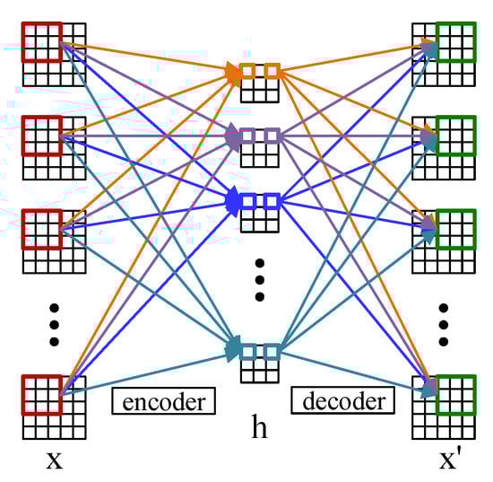
Figure 1.
The structure of the 2D convolutional autoencoder.
3. The Proposed Method
In this section, we will introduce our proposed method in detail. The flowchart is shown in Figure 2. Usually due to changes in atmospheric conditions, occlusion caused by the presence of clouds, changes in lighting, and other environmental disturbances, some noise bands in HSIs increase the difficulty in feature extraction and classification. As an unsupervised network, DFCEN is sensitive to these noise spectral bands because of the limited training samples and complex intrinsic features of HSIs. For this reason, a simple band selection based on mutual information is adopted for selecting and removing the noise bands at first. Then the relationships among samples is obtained for the specific learning task, which is specially based on LLE and LE in this paper. Next, training samples specifically applied to DFCEN are generated through a data preprocessing. Afterwards, DFCEN is learning from the training samples and relationship among samples. Eventually, the low-dimensional features from DFCEN is classified by classifiers.
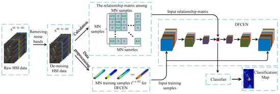
Figure 2.
Flowchart of the proposed method.
3.1. Data Preprocessing
Data preprocessing includes data standardization, data denoising and data expansion. Data standardization is to standardize the pixel values of each spectral band to 0∼1 since it is not appropriate to directly process the raw HSIs data with large pixel values. Data denoising is to select and remove the noise spectral band that may disturb feature extraction and classification. MI can evaluate the contribution of each band to classification [8], Besides, due to the simplicity of calculation, MI is adopted to search for bands that contribute little to the classification as the noise spectral band. Each band in HSIs is considered as a random variable. Its probability distribution function can be estimated as , where represents the gray-level histogram of the jth band with pixels. The joint probability distributions of any two bands in HSIs is estimated by , where is the joint gray-level histogram of the ith and jth band.
Figure 3 shows the MI values of each band in three datasets. As we can see, the two lines fluctuate almost identically. For this reason, we can find and remove noise bands with low MI in an unsupervised way according to the red dotted line. For a raw HSIs data , where M and N is the spatial size and is the raw number of the spectral bands, the corresponding de-noising data can be expressed as , where is the number of bands after removing the noise bands and . Actually, we only removed 30 noise bands for Indian Pines dataset, 0 band for Pavia University dataset, 8 bands for Salinas dataset. In order to further prove the validity of removing the noise bands before DFCEN, we take the Indian Pines dataset as an example to compare the classification accuracy of different dimensionality reduction algorithms before and after removing the noise bands. From Table 1, NBS means that the algorithm directly acts on the raw data while BS represents removing the noise bands before dimensionality reduction algorithm. It can be seen from Table 1 that for two unsupervised methods based on neural network, DFCEN and SAE, removing the noise bands is conducive to improving classification accuracy. In the meantime, it also slightly improves other dimensionality reduction algorithms.
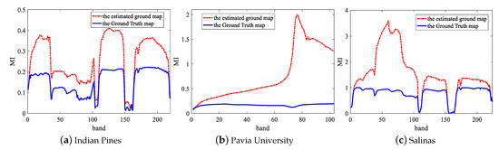
Figure 3.
MI values of each spectral band with the Ground Truth map and the estimated ground map on three datasets.

Table 1.
Classification accuracy of different dimensionality reduction (DR) algorithms with or without band selection for Indian Pines dataset.
Spatial features have been proven to be beneficial to improve the representation of HSIs and increase interpretation accuracy [35,36]. For each pixel, the neighborhood pixel is one of the most important spatial information which is fed to DFCEN in the form of neighborhood window centered around each pixel. With this in mind, the input data size of DFCEN is designed as , where s is the size of the neighborhood window and is the number of bands. However, the problem is that the neighborhood window of the pixels at the image boundary is incomplete. These boundary pixels cannot be ignored since our goal is to reduce the dimensions of each pixel in HSIs. It is also inappropriate to simply fill the neighborhood window of boundary pixels with 0. In order to deal with this problem better, we implement a data expansion strategy based on the Manhattan distance to fill the neighborhood window of the boundary pixels. Figure 4 shows the process of expanding the data by two layers, where the dark color is the original data and the light color is the filling data. For a pixel in a de-noising HSI ( is the number of pixels), its neighborhood window is a training sample that is fed to the proposed DFCEN. As a result, a training sample set with samples can be generated from a de-noising HSI .
Figure 4.
Data expansion strategy. This is the data expansion process when the size of neighborhood window is 5.
3.2. Structure of DFCEN
DFCEN is composed of convolutional layer and deconvolutional layer, excluding pooling layer and full-connected layer. Accordingly, DFCEN can be divided into two parts: convolutional subnetwork and deconvolutional subnetwork. In the convolutional subnetwork, the input data is propagated through multiple convolutional layers to a perception layer, while this perception layer is propagated through multiple deconvolutional layers to a output layer (whose size is same as the input layer) in the deconvolutional subnetwork.
Figure 5 shows the network structure of DFCEN. The introduction in the red box is the name and structure of each layer, while the name of the learning parameter and the filter size is in the green box. It is worth emphasizing that DFCEN is a symmetric and end-to-end network where the number of layers can be set or changed based on specific data or tasks. For the sake of explanation, we take a 7-layer DFCEN shown in Figure 5 as an example to introduce the network structure characteristics of DFCEN in detail. The following is the description of a 7-layer DFCEN shown in Figure 5.
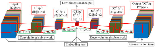
Figure 5.
The structure of the proposed deep fully convolutional embedding network.
In the convolutional subnetwork, firstly, a training sample is fed to DFCEN, where is also the number of channels of the input layer. Secondly, the output of input layer is sent to the first convolutional layer through filters of size . The output of contains feature maps that are then transmitted to the second convolutional layer via filters of size . Next, feature maps are obtained after is activated, which are then send to the last convolutional layer by d filters of size . The last convolutional layer in the convolutional subnetwork is also the central layer of the whole DFCEN. Eventually, a low-dimensional feature of concern is generated after applying the activation function to .
In the deconvolutional subnetwork, the low-dimensional feature (which is also the output of the convolutional subnetwork) from is up-sampled layer by layer through multiple deconvolutional layers. At first, is sent to the first deconvolutional layer with filters of size . Then, feature maps are gained after the activation function and then transfered to the second deconvolutional layer through filters of size . Next, after activating , feature maps are obtain and transfered to the last deconvolutional layer (which is also the output layer of the whole DFCEN) with filters size of . In the end, the output of the whole DFCEN is generated after is activated, whose size is the same as the input of DFCEN.
In fact, the characteristics of DFCEN are the size and number of filters (learning parameters), which are identical for the symmetrical layer in the convolutional and deconvolutional subnetwork. This rule also applies to the number and size of feature maps per layer. In particular, the number of feature maps per layer exists: where d is target dimension of dimensionality reduction and is the dimension of input data. Meanwhile, the relationship of the size of feature maps per layer is where s is the size of input data and the size of must be 1 since it represents the low-dimensional features of one pixel. For this reason, the size of the filter between and its preceding layer must be the same as the size of its preceding layer. In Figure 5, the preceding layer of is . In brief, DFCEN is a symmetric full convolutional network with a central layer of size 1, where the convolutional subnetwork reduce the dimensionality and size of data layer by layer while the deconvolutional subnetwork restores the data dimensionality and size layer by layer. Therefore, the network structure determines that feature extraction of DFCEN is an unsupervised process as long as the embedding term in objective function does not require any class label information.
3.3. Objective Function of DFCEN
As discussed in Section 1, DFCEN supports not only unsupervised feature extraction based on data reconstruction, but also task-specific learning which is conducive to dimensionality reduction and classification. The objective function of DFCEN consists of two terms: embedding term for the specific learning task and reconstruction term. The embedding term can be changed or designed according to specific concept or task, which is dedicated to improving the discriminant ability of the low-dimensional features. As shown in Figure 5, the embedding term is to constrain the low-dimensional output of the central layer . So it only acts on the parameter update of the convolutional subnetwork. For a training sample set , the output of in Figure 5 is expressed as follows
where is the learning parameters in the convolutional subnetwork. denotes the 2D convolution and is the activation function . is also the low-dimensional representation of DFCEN.
In order to enhance the separability and discriminability of low-dimensional features, we explore and maintain the relationship among samples as a specific learning task. In this paper, LLE and LE, two classical manifold learning algorithms are introduced into the embedding term of DFCEN.
3.3.1. LLE-Based Embedding Term
LLE aims at preserving the original reconstruction relationship between each sample and its neighbors in the mapping space, which assumes that a sample data can be reconstructed by a linear combination of its neighborhood samples. The linear reconstruction is described in Equation (2). The original reconstruction coefficient W can be calculated according to Equation (3). For a HSI dataset , the relationship coefficient W can be expressed as: . Since the coefficient W only characterizes the relationship between the sample and its nearest k neighbor samples, it can also be described as
is the nearest k neighbor samples of . The number of selected neighbor samples k is much smaller than the total number of samples , namely, . Therefore, the relationship coefficient matrix W is a sparse matrix.
Referring to LLE, the embedding term should constrain the low-dimensional representation to maintain the original reconstruction relationship. Hence, for a training sample set , the LLE-based embedding term can be defined as follow
where is the original reconstruction coefficient that is calculated according to Equation (11), which is a constant for the LLE-based embedding term. is the output of in DFCEN. is the learning parameters in the convolutional subnetwork. is the number of training samples in T. is the square of the F norm, which is to calculate the sum of the squares of all the elements inside.
3.3.2. LE-Based Embedding Term
LE is to construct the relationship among samples with local angels and reconstruct the local structure and features in the low-dimensional space. An adjacency graph based on the Euclidean distance is constructed to characterize the relationship among samples, which is also called the weight matrix and defined in Equation (6). When the sample does not belong to the nearest k neighbor samples of the sample , the weight coefficient between the samples and is 0. In fact, for a HSI dataset , due to , the adjacency graph matrix M is also a sparse matrix. In practice, LE hopes that samples that are related to each other (the points connected in the adjacency graph) are as close as possible in the low-dimensional space, which is described in a formula in Equation (5).
Referring to LE, for samples that are related in the original space, the embedding term should constrain their low-dimensional representation as close as possible. As a result, for a training sample set , the LE-based embedding term can be defined as follow
where is the adjacency graph coefficient in the original space, which also is a constant.
3.3.3. Reconstruction Term
As shown in Figure 5, the reconstruction term is to constrain the output of the whole DFCEN. So it acts on all learning parameter updates. The reconstruction term ensures that low-dimensional features can be restored as input data. For a training sample set , the output of DFCEN in Figure 5 is expressed as follow
where represents all learning parameters in DFCEN and is the parameters in the deconvolutional subnetwork. denotes the 2D deconvolution and is the activation function. is the output of the convolutional subnetwork.
The reconstruction term aims at maintaining original intrinsic information, which restores the low-dimensional features to the original input data. After the low-dimensional representation is propagated by the multiple deconvolutional layers, the reconstructed data q is obtained. The reconstruction term minimizes the error between the reconstructed data and the original input data. For a training sample set , the reconstruction term can be described as follow
where is the output of DFCEN and denotes all learning parameter.
3.3.4. Objective Function
The embedding and reconstruction term have been introduced above. The embedding term constrains the low-dimensional output of the central layer to maintain the original sample relationship, while the reconstruction term ensures that the low-dimensional feature is reconstructed back to the high-dimensional input data. To balance the effects of these two terms on dimensionality reduction, a trade-off parameter is added to the objective function. As a result, for a training sample set , the objective function of DFCEN can be described as
where is a adjustable trade-off parameter. is the reconstruction term and is the embedding term.
3.4. Learning of DFCEN
The learning of DFCEN is to optimize the network parameters according to the objective function which is formulated in Equation (16). In this paper, we adopt the gradient descent method to optimize learning parameters. The update formula for is expressed as , where is the partial derivative of the objective function with respect to , which has the form
In the following, we calculate these two partial derivatives separately. For a training sample , the partial derivative from the reconstruction term can be formulated as
Here is the partial derivative of the output layer (also last layer) with respect to all network parameters . For the 7-layer DFCEN shown in Figure 5, is the parameters in the convolutional subnetwork while is in the deconvolutional subnetwork. For , the partial derivative with respect to the lth layer parameters can be calculated as
where is the feature maps in the th layer and is the lth layer of DFCEN. When , is the input data . The derivation process can be consulted in [37]. represents a rotation of 180 degrees. is a 2D convolution. is the derivative function of the activation function, which is described as . For , the partial derivative is calculated as
where is a 2D deconvolution.
The embedding term is only responsible for updating the parameters in the convolutional subnetwork. For a training sample , the partial derivative of the LLE-based embedding term with respect to can be formulated as
Here is a constant. is the partial derivative of the central layer with to the parameters in the convolutional subnetwork. It can be expressed in the form of Equation (19). The partial derivative of the LE-based embedding term can be formulated as
where is also a constant.
In order to reduce the training time, we choose to use the convolutional autoencoder (CAE) to pretrain network to obtain good initial parameters. Owing to the symmetry of DFCEN, the parameter structure between the layers in the convolutional subnetwork is the same as that between the corresponding layers in the deconvolutional subnetwork. For this reason, symmetrical layers of two subnetworks can be initialized with the same parameters. So, a 7-layer DFCEN shown in Figure 5 only requires 3 CAEs for pretraining parameters, which saves the pretraining time. Figure 6 shows the pretraining process, where only after the first CAE has been trained can the second CAE be trained, and so on. The parameters in Figure 6, corresponding to the parameters in Figure 5, initializes DFCEN. The activation function of CAE is the same as that of DFCEN.
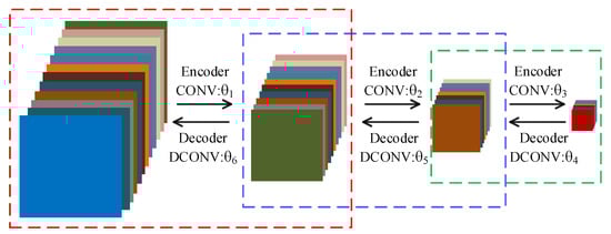
Figure 6.
Pretraining process. Each dashed box represents a convolutional autoencoder. correspond to the parameters in Figure 5.
4. Experimental Study
4.1. Description of Data Sets
The first dataset, Indian Pines Dataset, covering the Indian Pines region, northwest Indiana, USA, was acquired by the Airborne Visible/Infrared Imaging Spectrometer (AVIRIS) sensor in 1992. The spatial resolution of this image is 20 m. It has 220 original spectral bands in the 0.4–2.5 m spectral region and each band contains pixels. Owing to the noise and water absorption, 20 spectral bands are abandoned and the remaining 200 bands are used in this data set. This dataset contains background with 10,776 pixels and 16 ground-truth classes with 10,249 pixels. The number of pixels in each class is range from 20 to 2455. The color image and the labeled image with 16 classes are shown in Figure 7.
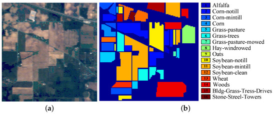
Figure 7.
Indian Pines dataset: (a) the color image, (b) the Ground Truth map.
The second dataset covers the University of Pavia, Northern Italy, which was acquired by the Reflective Optics System Imaging Spectrometer (ROSIS) sensor and called Pavia University Dataset. Its spectral range is 0.4–0.82 m. After removing 12 noise bands from the original dataset with 115 spectral bands, 103 bands are employed in this paper. The spatial resolution is 1.3 m and each band has pixels. This dataset consists of 9 ground-truth classes with 42,776 pixels and background with 164,624 pixels. Figure 8 shows the color image and the labeled image with 9 classes.
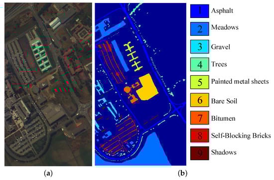
Figure 8.
Pavia University dataset: (a) the color image, (b) the Ground Truth map.
The third dataset, Salinas Dataset, covering Salinas Vally, CA, was acquired by AVIRIS sensor in 1998, whose spatial resolution is 3.7 m. There are 224 original bands with spectral ranging from 0.4 to 2.45 m. Each band has pixels including 16 ground-truth classes with 56,975 pixels and background with 54,129 pixels. After removing 20 bands that are severely affected by noise, the remaining 204 bands are used for the experiments. The color image and the labeled image with 16 classes are shown in Figure 9.
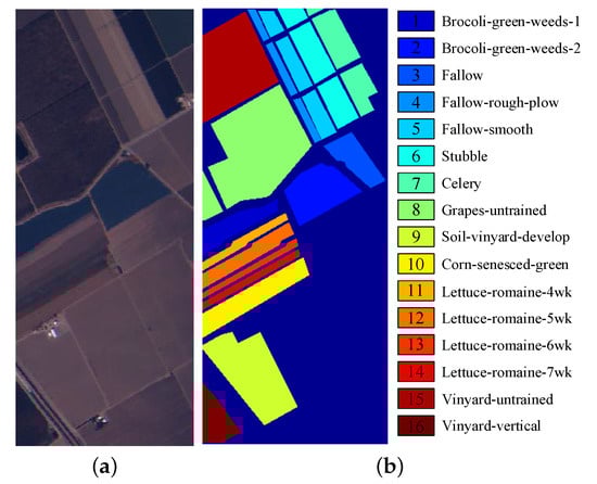
Figure 9.
Salinas dataset: (a) the color image, (b) the Ground Truth map.
4.2. Experimental Setup
For the sake of clarity, the proposed DFCEN with LLE-based embedding term is named DFCEN_LLE below while that with LE-based embedding term is written as DFCEN_LE. The network structure of DFCEN for three datasets is experientially designed on the basis of the structure of DFCEN described in Section 3.2. In this paper, DFCEN_LLE and DFCEN_LE have the same network structure for experimental convenience. The following is the network structure with a target dimensionality of 30. For the Indian Pines dataset, the network structure is 170–100–50–30–50–30–170 and the size of filter per layer is 3 × 3–2 × 2–2 × 2–2 × 2–2 × 2–3 × 3. For the Pavia University dataset, the network structure is 103–70–30–70–30–103 and the size of filer in all layers is . For the Salinas dataset, the network structure is 196–110–60–30–60–110–196 and the size of filer per layer is also .
To prove the effectiveness, DFCEN is compared with several dimensionality reduction algorithms, such as LE [11], LLE [11], SAE, spatial-domain local pixel NPE (LPNPE) [38], spatial and spectral regularized local discriminant embedding (SSRLDE) [38], SSMRPE [39], spatial–spectral local discriminant projection (SSLDP) [40]. The former three methods are spectral-based methods while the latter four approaches make use of both spatial and spectral information for dimensionality reduction of HSIs. Besides, the raw HSIs is also used for comparison. SAE is a algorithm based on neural network, and its network structures are 170–100–50–30–170 for Indian Pines dataset, 103–70–30–103 for Pavia University dataset, and 196–110–60–30–196 for Salinas dataset. LPNPE [38] minimizes the distance of the spatial local pixel neighborhood. SSRLDE [38] preserves not only the spectral-domain local Euclidean neighborhood class relations but also the spatial-domain local pixel neighborhood structures. SSMRPE [39] shares the same DR concept as LLE. SSLDP [40] designs a weighted within neighborhood scatter to reveal the similarity of spatial neighbors. Among them, SSRLDE [38] and SSLDP [40] are supervised and require class labels to implement dimensionality reduction, while others are unsupervised.
For the fairness of the experimental comparison, the numbers of the nearest neighbor samples k of LE and LLE are the same as that of DFCEN_LE and DFCEN_LLE in the following experiments. We also choose the optimal parameters of their source literature for LPNPE [38], SSRLDE [38], SSMRPE [39], SSLDP [40]. In all the experiments below, all algorithms including DFCEN use raw data (that is not filtered to de-noise and smoothen pixels). For this reason, the results of the comparative experiments in this paper are different from those in the source literature (they usually use de-noising and smooth pixels).
Moreover, two classifiers support vector machines (SVM) and k nearest neighbor (KNN) are employed for classifying dimensionality reduction results. In fact, the number of the nearest neighbor of KNN is equal to 1. In all experiments, we randomly divide each HSI dataset into training and test sets. It should be emphasized that the training set is used to train the dimensionality reduction models and classifiers for supervised algorithms while that is only used to train classifiers for unsupervised algorithms. Actually, all samples in a HSI dataset are utilized to train the dimensionality reduction models for unsupervised methods. Overall classification accuracy (OA), average classification accuracy (AA), and the kappa coefficient are used to evaluate classification performance. To robustly evaluate the results with different dimensionality reduction algorithms, we repeat 10 times for each experiment.
4.3. Parameters Analysis
Both DFCEN_LE and DFCEN_LLE have three parameters that need to be set manually, including nearest neighbor number k, spatial window size s and trade-off parameter . In order to analyze the influence of three parameters on dimensionality reduction, we conduct parameter tuning experiments on three HSI datasets. in each class are randomly selected as the training set and the remaining samples are the testing set for two classifiers. Figure 10 shows the classification accuracy from DFCEN with different parameters on Indian Pines dataset, where the parameter range is set to: , , and the fixed values are set to , , to analyze the other two parameters.
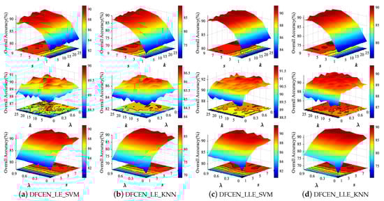
Figure 10.
Classification overall accuracy with respect to different parameters of deep fully convolutional embedding network (DFCEN) on Indian Pines dataset from two classifiers.
From Figure 10, the effects of the three parameters on DFCEN_LE and DFCEN_LLE are almost the same. The classification accuracy increases significantly with the increase of s when k or is fixed, which means that spatial information is important for DR. But the classification accuracy tends to decline when s continues to increase, because the large spatial window may contain heterogeneous samples which interfere with the extraction of spatial homogeneous information. Meanwhile, the classification accuracy increases with the increase of and k when s is fixed. In particular, the change of from zero has led to a significant improvement in classification, which proves that the specific learning task (this is embodied in the embedding term) of exploring and preserving the relationships among samples can effectively enhance the discriminability and separability of low-dimensional features and the proposed DFCEN is meaningful. Through a simple parameter tuning experiment, the three parameters of DFCEN_LE and DFCEN_LLE on the three datasets are set as shown in Table 2.
Table 2.
Three parameter Settings for DFCEN_LE and DFCEN_LLE on three datasets.
4.4. Convergence and Discriminant Analysis
To illustrate the convergence of DFCEN, the learning curves of the embedding and reconstruction terms of DFCEN_LLE and DFCEN_LE on three datasets are present in Figure 11, in which the parameters have been initialized by CAEs. The x-axis represents the number of learning parameter updates that are performed after learning each batch of samples (a batch contains 50 samples). The curve represents the error values of two terms in objective function after one iteration (namely, all samples have been learned). (a)–(c) and (g)–(i) is about DFCEN_LLE, where two terms on three datasets all can remain convergent and obtain small error values after repeated iterations. (d)–(f) and (j)–(l) is about DFCEN_LE. From that, the error values of two terms on the Indian Pines and Salinas datasets can remain consistently convergent as the number of iterations increases. However, the error values of the reconstruction term in the early learning stage on the Pavia University dataset does not converge but increases. The reason is probably high trade-off parameter ( shown in Table 2) and overfitting occurred in pretraining where the objective function of CAEs is consistent with the reconstruction term. Nevertheless, two terms on the Pavia University dataset eventually converge to a small error value as the number of iterations increases. Accordingly, DFCEN_LLE and DFCEN_LE can achieve a good convergence, from which the low-dimensional features not only preserves the original relationship among samples, but also retains the original intrinsic information in HSIs.
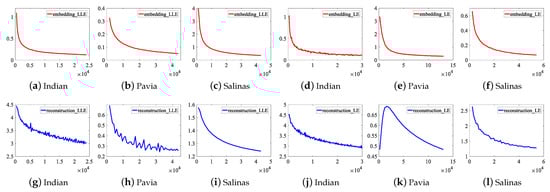
Figure 11.
The learning curves of the embedding and reconstruction terms of DFCEN_LLE and DFCEN_LE on three datasets.
To analyze the discriminability and separability of the low-dimensional features from DFCEN, t-SNE is used to visualize the low-dimensional data of DFCEN comparing the raw data. The 2-dimensional features obtained by t-SNE on three datasets are shown in Figure 12 where different colors stand for different classes. Figure 12 shows all class samples for the Indian Pines and Pavia University datasets and randomly 80% for the Salinas dataset due to the large number of the class samples. As we can observe from these visualizations, the dimensionality reduction results from DFCEN are more discriminative than the raw HSIs data. Owing to DFCEN, the separability among different classes in the low-dimensional space is significantly improved compared to the original space. The reason is that DFCEN not only maintains the original intrinsic information but also preserves the original relationship among samples. In particular, DFCEN_LLE preserves the original reconstructed relationship between each sample and its k nearest neighbors, while DFCEN_LE keeps each sample as close as possible to its k nearest neighbors, since there is a high probability that each sample and its neighbor belong to the same class. As a result, from Figure 12, the same classes from DFCEN are clustered together and the different classes are effectively separated.
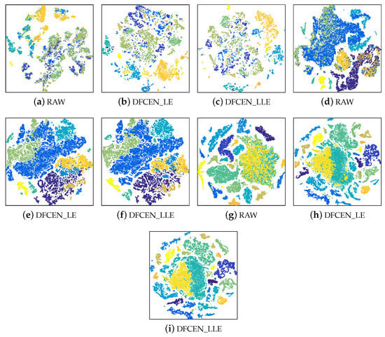
Figure 12.
The two-dimensional features obtained by t-SNE from the raw data and the low-dimensional features of DFCEN on three datasets: (a–c) Indian Pines, (d–f) Pavia University, (g–i) Salinas.
4.5. Classification Performance
In this subsection, we examine the classification performance of dimensionality reduction results on three datasets. SVM and KNN are used to classify dimensionality reduction results to reduce the influence of classifiers. Firstly, in order to analyze the classification performance under different classification conditions, we randomly selected 5%, 10% and 15% of samples from each class as training set, and other samples are tested. The training set and test set are applied to all algorithms in the manner described in Section 4.2.
Table 3 shows the overall classification accuracy of the dimensionality reduction results (dim = 30) from different algorithms on three datasets, where the OA values is the average of 10 experiments under the same classification conditions. From Table 3, we can see that the classification OA values of all dimensionality reduction algorithms improve as the proportion of training samples increases since more training data can provide more class information for classifiers and supervised dimensionality reduction algorithms. The highest OA value under the same classification condition has been marked in bold.
Table 3.
Classification accuracy of dimensionality reduction results (dim = 30) of different algorithms using SVM and KNN classifiers with different proportions of training samples on three datasets.
As we have seen, the spatial–spectral combined algorithm, LPNPE [38], SSRLDE [38], SSMRPE [39], SSLDP [40] and DFCEN, are superior to the spectral-based algorithm, LE, LLE and SAE, which indicates that spatial features are beneficial to the dimensionality reduction of HSIs. Neural network based methods, SAE and DFCEN, are superior to traditional dimensionality reduction algorithms, which testifies that neural network is suitable for dimensionality reduction of HSIs. Compared with other algorithms in this paper, the dimensionality reduction results of DFCEN has the best classification performance for three datasets under two classifiers. In particular, DFCEN achieves superior classification accuracy even with only 5% of the training samples of classifiers.
Secondly, in order to analyze the classification performances per class of different algorithms, 10% of samples per class are randomly selected as training samples and others are as test samples. The individual class classification accuracy, OA, AA, and on three datasets are shown in Table 4, Table 5 and Table 6. The highest value of each item has been marked in bold. Figure 13, Figure 14 and Figure 15 show the corresponding classification maps of different algorithms on three datasets. From Table 4, Table 5 and Table 6, the supervised algorithms, SSRLDE and SSLDP, give unsatisfactory classification results in Indian Pines and Pavia University datasets due to the absence of pixel filtering, which indicates that SSRLDE and SSLDP are very sensitive to noise pixels. Meanwhile, as two unsupervised algorithms, DFCEN_LLE and DFCEN_LE achieved the highest classification accuracy in most classes, even with OA, AA and achieving the best. Especially for class 9 in Indian Pines, class 3 in Pavia and class 15 in Salinas, DFCEN obtain high classification accuracy while other algorithms are poor because of the difficulty in classifying these classes. In terms of OA, DFCEN is approximately 4% better than that of the second best algorithm.
Table 4.
Classification accuracy of each class (DIM = 30) for Indian Pines datasets via SVM and KNN classifiers.
Table 5.
Classification accuracy of each class (DIM = 30) for Pavia University datasets via SVM and KNN classifiers.
Table 6.
Classification accuracy of each class (DIM = 30) for Salinas datasets via SVM and KNN classifiers.
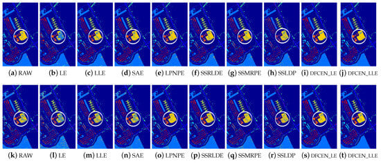
Figure 13.
Classification maps with two classifiers of different methods on the University of Pavia dataset (dim = 30). (a–j) are for KNN and (k–t) are for SVM. (i,j) and (s,t) are the classification result of DFCEN.
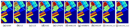
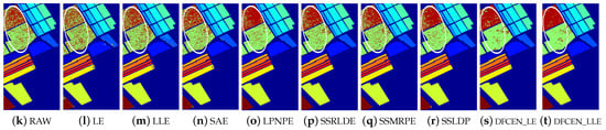
Figure 14.
Classification maps with two classifier of different methods on Salinas data set (dim = 30). (a–j) are for KNN and (k–t) are for SVM. (i,j) and (s,t) are the classification result of the proposed DFCEN.
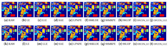
Figure 15.
Classification maps of different methods on Indian Pines dataset (dim = 30) via two classifiers. (a–j) are for k nearest neighbor (KNN) and (k–t) are for support vector machines (SVM). (i,j) and (s,t) are the classification result of DFCEN.
Figure 13, Figure 14 and Figure 15 visually show the classification maps of the DR results (DIM = 30) of different algorithms. From that, it can be observed that DFCEN has significant regional classification uniformity because DFCEN not only guarantees the intrinsic information of HSIs but also explores and maintains the relationship among samples and their nearest neighbors. Especially for classes 3, 9, 10, 12, and 15 of the Indian Pines dataset, classes 6 and 7 of the Pavia University dataset, and classes 8 and 15 of the Salinas dataset (these classes have been circled in white in Figure 13, Figure 14 and Figure 15, DFCEN performs much better than the other methods under two classifiers.
Thirdly, to analyze the influence of different dimensions on each algorithm, Figure 16 shows the changes of OA with two classifiers on three datasets when the dimensionality ranges from 5 to 50 with the step length of 5. From that, the OAs of most algorithms improve with the increase of dimensions and tend to be stable when the dimension increases to a certain degree. The reason is that the higher the feature dimension is, the more information it can provide for the classification, but it will reach saturation when the feature dimension continues to increase. Moreover, in Figure 16, spatial–spectral DR methods, LPNPE, SSRLDE, SSMRPE, SSRLDE and DFCEN, are generally superior to spectral-based methods, LE, LLE and SAE. In particular, DFCEN achieves almost the best classification on the results of different dimensions compared with other algorithms.
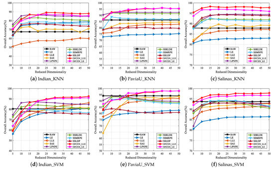
Figure 16.
Classification overall accuracy of reduced dimensionality (DIM = 5∼50) on three datasets with SVM and KNN classifiers.
Figure 16 also shows that the classification OAs of LE and LLE are relatively poor. However, DFCEN_LE and DFCEN_LLE have satisfactory classification performance when the concepts of LE and LLE are introduced to DFCEN. The reason may be summarized as follows: (1) the fully convolutional network of DFCEN can effectively obtain the spatial–spectral information of HSIs by layer-by-layer feature extraction, (2) the reconstruction term, as a regularization term corresponding to the embedding term, can constrain low-dimensional features to retain the intrinsic information.
5. Conclusions
In this paper, a novel unsupervised DFCEN was proposed for HSIs dimensionality reduction. Different from the existing unsupervised CNN-based method which only focuses on data reconstruction, DFCEN was designed to not only ensure data reconstruction but also realize the learning of specific tasks. In DFCEN, convolutional subnetwork is for dimensionality reduction and specific task learning while deconvolutional subnetwork is for data reconstruction. A novel objective function was proposed, including two terms: embedding term of the specific task and reconstruction term of data reconstruction. The former enhance the discriminant ability of low-dimensional features and the latter maintain the original intrinsic information. In this paper, exploring and maintaining relationships between samples as a specific task to improve dimensionality reduction performance, while the dimensionality reduction concepts of LLE and LE are introduced into DFCEN. Experimental results on three hyperspectral datasets prove the superior classification performance of the dimensionality reduction results from DFCEN_LLE and DFCEN_LE.
In our future work, different dimensionality reduction concepts and objective functions designed according to specific requirements will be applied to DFCEN to achieve DR and the idea of the combination of LE and LLE will be tried. In addition, we will try to apply DFCEN to other areas.
Author Contributions
Conceptualization, N.L. and M.Z.; methodology, N.L.; software, N.L.; validation, N.L., M.Z. and T.W.; formal analysis, N.L.; investigation, N.L.; resources, D.Z.; data curation, J.S.; writing—original draft preparation, N.L.; writing—review and editing, N.L.; visualization, N.L.; supervision, M.G.; project administration, D.Z.; funding acquisition, J.S. All authors have read and agreed to the published version of the manuscript.
Funding
This work was supported in part by National Natural Science Foundation of China (Grant No. 62076204), the National Natural Science Foundation of Shaanxi Province under Grantnos. 2018JQ6003 and 2018JQ6030, the China Postdoctoral Science Foundation (Grant nos. 2017M613204 and 2017M623246).
Data Availability Statement
Not applicable.
Conflicts of Interest
The authors declare no conflict of interest.
References
- Murphy, R.J.; Monteiro, S.T.; Schneider, S. Evaluating Classification Techniques for Mapping Vertical Geology Using Field-Based Hyperspectral Sensors. IEEE Trans. Geosci. Remote Sens. 2012, 50, 3066–3080. [Google Scholar] [CrossRef]
- Ryan, J.P.; Davis, C.O.; Tufillaro, N.B.; Kudela, R.M.; Gao, B.C. Application of the hyperspectral imager for the coastal ocean to phytoplankton ecology studies in Monterey Bay, CA, USA. Remote Sens. 2014, 6, 1007–1025. [Google Scholar] [CrossRef]
- Pi, W.; Du, J.; Liu, H.; Zhu, X. Desertification Glassland Classification and Three-Dimensional Convolution Neural Network Model for Identifying Desert Grassland Landforms with Unmanned Aerial Vehicle Hyperspectral Remote Sensing Images. J. Appl. Spectrosc. 2020, 87, 309–318. [Google Scholar] [CrossRef]
- Ofner, J.; Kamilli, K.A.; Eitenberger, E.; Friedbacher, G.; Lendl, B.; Held, A.; Lohninger, H. Chemometric analysis of multisensor hyperspectral images of precipitated atmospheric particulate matter. Anal. Chem. 2015, 87, 9413–9420. [Google Scholar] [CrossRef] [PubMed]
- de la Ossa, M.Á.F.; Amigo, J.M.; García-Ruiz, C. Detection of residues from explosive manipulation by near infrared hyperspectral imaging: A promising forensic tool. Forensic Sci. Int. 2014, 242, 228–235. [Google Scholar] [CrossRef]
- Guo, X.; Huang, X.; Zhang, L.; Zhang, L. Hyperspectral image noise reduction based on rank-1 tensor decomposition. ISPRS J. Photogramm. Remote Sens. 2013, 83, 50–63. [Google Scholar] [CrossRef]
- Jia, X.; Kuo, B.C.; Crawford, M.M. Feature Mining for Hyperspectral Image Classification. Proc. IEEE 2013, 101, 676–697. [Google Scholar] [CrossRef]
- Guo, B.; Gunn, S.R.; Damper, R.I.; Nelson, J.D.B. Band Selection for Hyperspectral Image Classification Using Mutual Information. IEEE Geosci. Remote Sens. Lett. 2006, 3, 522–526. [Google Scholar] [CrossRef]
- Hughes, G. On the mean accuracy of statistical pattern recognizers. IEEE Trans. Inf. Theory 1968, 14, 55–63. [Google Scholar] [CrossRef]
- Li, Y.; Qu, J.; Dong, W.; Zheng, Y. Hyperspectral pansharpening via improved PCA approach and optimal weighted fusion strategy. Neurocomputing 2018, 315, 371–380. [Google Scholar] [CrossRef]
- Belkin, M.; Niyogi, P. Laplacian eigenmaps for dimensionality reduction and data representation. Neural Comput. 2003, 15, 1373–1396. [Google Scholar] [CrossRef]
- Li, W.; Zhang, L.; Zhang, L.; Du, B. GPU parallel implementation of isometric mapping for hyperspectral classification. IEEE Geosci. Remote Sens. Lett. 2017, 14, 1532–1536. [Google Scholar] [CrossRef]
- Bandos, T.V.; Bruzzone, L.; Camps-Valls, G. Classification of Hyperspectral Images With Regularized Linear Discriminant Analysis. IEEE Trans. Geosci. Remote Sens. 2009, 47, 862–873. [Google Scholar] [CrossRef]
- He, X.; Niyogi, P. Locality preserving projections. In Advances in Neural Information Processing Systems; The MIT Press: Cambridge, MA, USA, 2004; pp. 153–160. [Google Scholar]
- He, X.; Cai, D.; Yan, S.; Zhang, H.J. Neighborhood preserving embedding. In Proceedings of the Tenth IEEE ICCV, Beijing, China, 17–20 October 2005; Volume 2, pp. 1208–1213. [Google Scholar]
- Han, T.; Goodenough, D.G. Investigation of Nonlinearity in Hyperspectral Imagery Using Surrogate Data Methods. IEEE Trans. Geosci. Remote Sens. 2008, 46, 2840–2847. [Google Scholar] [CrossRef]
- Bengio, Y.; Courville, A.C.; Vincent, P. Unsupervised feature learning and deep learning: A review and new perspectives. CoRR 2012, 1, 2012. [Google Scholar]
- Paoletti, M.E.; Haut, J.M.; Plaza, J.; Plaza, A. Deep learning classifiers for hyperspectral imaging: A review. ISPRS J. Photogramm. Remote Sens. 2019, 158, 279–317. [Google Scholar] [CrossRef]
- Paoletti, M.; Haut, J.; Plaza, J.; Plaza, A. A new deep convolutional neural network for fast hyperspectral image classification. ISPRS J. Photogramm. Remote Sens. 2018, 145, 120–147. [Google Scholar] [CrossRef]
- Zhong, Z.; Li, J.; Luo, Z.; Chapman, M. Spectral–spatial residual network for hyperspectral image classification: A 3-D deep learning framework. IEEE Trans. Geosci. Remote Sens. 2017, 56, 847–858. [Google Scholar]
- Han, M.; Cong, R.; Li, X.; Fu, H.; Lei, J. Joint spatial-spectral hyperspectral image classification based on convolutional neural network. Pattern Recognit. Lett. 2020, 130, 38–45. [Google Scholar] [CrossRef]
- Mou, L.; Ghamisi, P.; Zhu, X.X. Unsupervised spectral–spatial feature learning via deep residual Conv–Deconv network for hyperspectral image classification. IEEE Trans. Geosci. Remote Sens. 2017, 56, 391–406. [Google Scholar] [CrossRef]
- Zhang, M.; Gong, M.; Mao, Y.; Li, J.; Wu, Y. Unsupervised feature extraction in hyperspectral images based on wasserstein generative adversarial network. IEEE Trans. Geosci. Remote Sens. 2018, 57, 2669–2688. [Google Scholar] [CrossRef]
- Zhang, M.; Gong, M.; He, H.; Zhu, S. Symmetric All Convolutional Neural-Network-Based Unsupervised Feature Extraction for Hyperspectral Images Classification. IEEE Trans. Cybern. 2020. [Google Scholar] [CrossRef]
- Estévez, P.A.; Tesmer, M.; Perez, C.A.; Zurada, J.M. Normalized mutual information feature selection. IEEE Trans. Neural Netw. 2009, 20, 189–201. [Google Scholar] [CrossRef]
- Chang, C.I.; Kuo, Y.M.; Chen, S.; Liang, C.C.; Ma, K.Y.; Hu, P.F. Self-Mutual Information-Based Band Selection for Hyperspectral Image Classification. IEEE Trans. Geosci. Remote. Sens. 2020. [Google Scholar] [CrossRef]
- Pan, Y.; Ge, S.S.; Al Mamun, A. Weighted locally linear embedding for dimension reduction. Pattern Recognit. 2009, 42, 798–811. [Google Scholar] [CrossRef]
- Roweis, S.T.; Saul, L.K. Nonlinear dimensionality reduction by locally linear embedding. Science 2000, 290, 2323–2326. [Google Scholar] [CrossRef]
- Wang, M.; Yu, J.; Niu, L.; Sun, W. Unsupervised feature extraction for hyperspectral images using combined low rank representation and locally linear embedding. In Proceedings of the 2017 IEEE ICASSP, New Orleans, LA, USA, 5–9 March 2017; pp. 1428–1431. [Google Scholar]
- Li, B.; Li, Y.R.; Zhang, X.L. A survey on Laplacian eigenmaps based manifold learning methods. Neurocomputing 2019, 335, 336–351. [Google Scholar]
- Ma, M.; Deng, T.; Wang, N.; Chen, Y. Semi-supervised rough fuzzy Laplacian Eigenmaps for dimensionality reduction. Int. J. Mach. Learn. Cybern. 2019, 10, 397–411. [Google Scholar] [CrossRef]
- Seyfioğlu, M.S.; Özbayoğlu, A.M.; Gürbüz, S.Z. Deep convolutional autoencoder for radar-based classification of similar aided and unaided human activities. IEEE Trans. Aerosp. Electron. Syst. 2018, 54, 1709–1723. [Google Scholar] [CrossRef]
- Azarang, A.; Manoochehri, H.E.; Kehtarnavaz, N. Convolutional autoencoder-based multispectral image fusion. IEEE Access 2019, 7, 35673–35683. [Google Scholar] [CrossRef]
- Palsson, B.; Ulfarsson, M.O.; Sveinsson, J.R. Convolutional Autoencoder for Spectral–Spatial Hyperspectral Unmixing. IEEE Trans. Geosci. Remote Sens. 2020, 59, 535–549. [Google Scholar]
- Fauvel, M.; Tarabalka, Y.; Benediktsson, J.A.; Chanussot, J.; Tilton, J.C. Advances in spectral-spatial classification of hyperspectral images. Proc. IEEE 2013, 101, 652–675. [Google Scholar] [CrossRef]
- Plaza, A.; Martínez, P.; Pérez, R.; Plaza, J. Spatial/spectral endmember extraction by multidimensional morphological operations. IEEE Trans. Geosci. Remote Sens. 2002, 40, 2025–2041. [Google Scholar] [CrossRef]
- Bouvrie, J. Notes on Convolutional Neural Networks. Available online: http://cogprints.org/5869/ (accessed on 13 February 2021).
- Zhou, Y.; Peng, J.; Chen, C.P. Dimension reduction using spatial and spectral regularized local discriminant embedding for hyperspectral image classification. IEEE Trans. Geosci. Remote Sens. 2014, 53, 1082–1095. [Google Scholar] [CrossRef]
- Huang, H.; Shi, G.; He, H.; Duan, Y.; Luo, F. Dimensionality reduction of hyperspectral imagery based on spatial-spectral manifold learning. IEEE Trans. Cybern. 2019, 50, 2604–2616. [Google Scholar] [CrossRef] [PubMed]
- Huang, H.; Duan, Y.; He, H.; Shi, G.; Luo, F. Spatial-spectral local discriminant projection for dimensionality reduction of hyperspectral image. ISPRS J. Photogramm. Remote Sens. 2019, 156, 77–93. [Google Scholar] [CrossRef]


Publisher’s Note: MDPI stays neutral with regard to jurisdictional claims in published maps and institutional affiliations. |
© 2021 by the authors. Licensee MDPI, Basel, Switzerland. This article is an open access article distributed under the terms and conditions of the Creative Commons Attribution (CC BY) license (http://creativecommons.org/licenses/by/4.0/).