A Detection of Convectively Induced Turbulence Using in Situ Aircraft and Radar Spectral Width Data

Abstract

A commercial aircraft, departing from Seoul to Jeju Island in South Korea, encountered a convectively induced turbulence (CIT) at about z = 2.2 km near Seoul on 28 October 2018. At this time, the observed radar reflectivity showed that the convective band with cloud tops of z = 6–7 km passed the CIT region with high values of spectral width (SW; larger than 4 m s^–1). Using the 1 Hz wind data recorded by the aircraft, we estimated an objective intensity of the CIT as a cube root of eddy dissipation rate (EDR) based on the inertial range technique, which was about 0.33–0.37 m^2/3 s⁻¹. Radar-based EDR was also derived by lognormal mapping technique (LMT), showing that the EDR was about 0.3–0.35 m^2/3 s⁻¹ near the CIT location, which is consistent with in situ EDR. In addition, a feasibility of the CIT forecast was tested using the weather and research forecast (WRF) model with a 3 km horizontal grid spacing. The model accurately reproduced the convective band passing the CIT event with an hour delay, which allows the use of two methods to calculate EDR: The first is using both the sub-grid and resolved turbulent kinetic energy to infer the EDR; the second is using the LMT for converting absolute vertical velocity (and its combination with the Richardson number) to EDR-scale. As a result, we found that the model-based EDRs were about 0.3–0.4 m^2/3 s⁻¹ near the CIT event, which is consistent with the estimated EDRs from both aircraft and radar observations.

1. Introduction

Atmospheric turbulence in the free atmosphere is one of the most dangerous aviation weather hazards, as it can cause in-flight injuries and fatalities, and structural damage, shortening the longevity of aircraft and causing flight delays and fuel losses [1,2,3]. Turbulence directly affecting aircraft in the free atmosphere is classified into three types depending on its generation mechanism and location: Clear-air turbulence (CAT), mountain wave turbulence (MWT), and convectively induced turbulence (CIT) [2,3,4,5,6,7]. CAT can be induced by shear instability above and below the upper-level jet core [8,9,10], inertia instability in anticyclonic shear and curved flows [11,12,13], and inertia gravity waves and their subsequent triggers near the exit region of the jet or above the jet core [14,15]. MWT is associated with a propagation of mountain waves, encountering a critical level, and a breaking of mountain waves [2,3,6,7,9,16,17,18]. CIT can occur both within and out of clouds, which are called in-cloud CIT and out-of-cloud CIT, respectively. The strong updraft and downdraft within a convective cloud and the flow deformation induced by the overshooting of the convection cause strong jolts to aircrafts [19,20,21]. Convective gravity waves (CGWs) can generate out-of-cloud CIT, which is referred to as near-cloud turbulence (NCT), both above or laterally away from the main convection through the CGW propagation, critical-level filtering, and/or its breaking [20,21,22,23,24,25,26]. Horizontal convective rolls within cirrus bands can also provide an environment conducive to NCT through thermal-shear instability [13,25].

In general, the prediction of atmospheric turbulence for aviation operations has been developed through two approaches: Forecast and nowcast, which have been used in strategical and tactical flight route planning [3,27,28,29,30]. For forecast systems (for strategical planning), numerical weather prediction (NWP) models are used to predict CAT and MWT because several NWP-based turbulence diagnostics have been developed and formulated to capture the large-scale forces, such as upper-level jets, fronts, and background flows conducive to mountain waves, which are well-resolved even in coarser grid spacings. Accordingly, the current operational forecast systems for aviation turbulence, such as Graphical Turbulence Guidance (GTG) [27,30] and Korean Turbulence Guidance (KTG) [31,32], have focused on predicting CAT and MWT based on the NWP-based CAT and MWT diagnostics by considering the energy of those large-scale disturbance cascades down to small-scale turbulent eddies [33,34]. These turbulence diagnostics are calibrated in terms of the cube root of the eddy dissipation rate (EDR, in m^2/3 s⁻¹), which is the International Civil Aviation Organization (ICAO) standard metric used for turbulence reporting and measurement [3,27,28,29,30,35,36,37].

The nowcast system (for tactical planning) is focused on CIT. Achieving precise CIT forecast is challenging using the current and near-future version of the NWP model because convection is short-lived, instantaneous, and transient. It is difficult to predict the resultant CIT based on the current spatiotemporal resolution of the underlying operational NWP models. To overcome the current limitations in CIT forecasting, several previous studies have used remote sensing (i.e., radar and satellite) data [28,38]. The seamless combination of remote sensing-based convection and NWP-based turbulence forecasting is useful for aviation operations. Over the contiguous United States, authors [38] developed a turbulence-nowcasting algorithm to produce an EDR-scale turbulence output by combining the NWP-based turbulence diagnostics (e.g., convective available potential energy, turbulent kinetic energy (TKE), and vertical velocity) and radar-based products (e.g., radar reflectivity, echo top, and spectral width (SW)). They also used other observational data such as terminal weather reports on wind speed and gust observation, pilot reports of turbulence (PIREPs), and in situ aircraft data to produce the EDR nowcasts. They found that the turbulence forecasting ability was improved when the abovementioned observational data were incorporated and blended with the NWP-based products.

As a baseline study for the development of a CIT forecast system in South Korea, we examined the CIT event on 28 October 2018 in South Korea, and estimated the EDRs using in situ aircraft data, Doppler radar-based SW data, and convection-permitting numerical simulation results. This paper is organized as follows: In Section 2, we provide an overview of the observed CIT event and its EDR value from the aircraft data. In Section 3, the EDR is derived from the radar SW data and it is compared with in situ aircraft-based EDR. In Section 4, we conduct a convection-permitting numerical simulation on the CIT event and estimate the model-based EDRs. In Section 5, discussions on the predictability of CIT under the current physical and dynamical settings of the model are provided. A summary is provided in the last section.

2. Case Investigation

2.1. In Situ Aircraft Data

On 28 October 2018, a commercial aircraft departing from Seoul, Gimpo International Airport (37.59°N, 126.63°E) and heading to Jeju International Airport, South Korea (Figure 1) encountered turbulence during takeoff (near 05:42 UTC) at a flight level of 7173 ft (z = 2.2 km above the ground level (AGL)). At this time, it was located within a cloud band along with a cold front moving toward the Korean peninsula, which will be shown later in Section 2.2 with radar images. To estimate the objective intensity of the CIT event, we used the in situ aircraft quick access recorder (QAR) data with a 1 Hz sampling rate. The QAR records position (longitude, latitude, and altitude), vertical acceleration (in units of g, where g is the gravitational acceleration) of the aircraft, and meteorological variables such as wind speed and direction and air temperature.

Figure 2 shows the time series of vertical acceleration, wind speed and direction, and altitude during the entire period of the flight route shown in Figure 1, starting from the gate at Gimpo at 05:26 UTC to the gate at Jeju at 06:38 UTC on 28 October 2018. At 05:42 UTC, immediately after take-off, the aircraft encountered the CIT, and deviation in vertical acceleration per second (Δg) was more than 1 g, from 0.277 to 1.5 g, which corresponds to moderate-intensity turbulence by the ICAO definition [36,37]. While a prevailing westerly wind was dominant with a steady value of 270 degrees from the north (green line at upper panel of Figure 2), there were very strong fluctuations in both wind speed and direction in the QAR data at this time (highlighted in yellow in Figure 2). Fortunately, there were no inflight injuries or damage because all crew members and passengers had fastened their seat belts during the take-off period (personal communication with Captain Kim in 2020). With other avionic parameters such as pitch and roll angles from the QAR data (not shown), it is also confirmed that the fluctuations were mainly because of turbulence with minor impact by changing altitudes of the airplane.

Using the 3000 data samples of the QAR data from 05:40 UTC to 06:30 UTC on 28 October 2018, horizontal wind components are directly compared with the fifth generation of the European Centre for Medium-range Weather Forecast reanalysis (ERA5) data with 0.25 × 0.25 degree of horizontal grid resolution (Figure 3). Results showed that wind data from the QAR is similar to the ERA5 data with the mean absolute error (MAE) of 1.81–2.03 m s⁻¹ and root mean square error (RMSE) of 2.55–2.85 m s⁻¹, which are within a typical range of observation error by aircraft data [39]. Using the recorded variables in the QAR data, we estimated an objective magnitude of turbulence intensity as a function of EDR, which is the cube root of energy dissipation rate of TKE in the atmosphere. Many previous studies have been conducted to estimate the EDR using flight measurements [40,41,42,43]. In the current study, EDR was calculated using the QAR variables based on the inertial range technique (IRT) [43,44,45]. The IRT is based on the Kolmogorov energy spectrum in the inertial subrange at which TKE is converted to the heat, and the turbulent eddies showing a 3D isobaric feature [46,47]. In the inertial subrange, the power spectral density (PSD) follows a power law with a slope of k^−5/3 (where k is zonal wavenumber) and depends on the eddy dissipation rate (ε), which is expressed as a function of zonal wavenumber k:

E(k) = Cε^2/3k^−5/3,

(1)

where, E(k) is the PSD for the zonal wind component and C is the Kolmogorov constant, which was set to 0.53 in this study. Here, EDR was estimated using Kolmogorov’s law (i.e., inertial range slope) and Taylor’s frozen hypothesis [43,44,45,46,47,48,49], as follows:

$$\mathrm{EDR}={\mathsf{\epsilon }}^{1/3}={\left(\frac{2\pi }{V}\right)}^{1∕3}{\left[\frac{\overline{s_u\left(f\right)f^{5∕3}}}{C^{-1}}\right]}^{\raisebox{1ex}{$1$}\!\left/ \!\raisebox{-1ex}{$2$}\right.}$$

(2)

where V is averaged airspeed of aircraft for a given time window, which was 120 s in this study; $S_u\left(f\right)$ is the PSD in the frequency (f) domain; and overbar is the average values within the defined inertial subrange (0.1–0.5 s⁻¹). PSD was estimated by the fast Fourier transform (FFT) with no window. For a given time window (2 min), one PSD was calculated. Then, the time window moved every second from the start to the end of the entire flight time, so that we obtained the PSD and subsequent EDR for every second. Finally, the estimated EDRs were averaged for every 30 s, which were the cube root of ε in m^2/3 s⁻¹.

Figure 4 shows some examples of the calculated PSDs for zonal wind from the QAR data recorded during the CIT event. It also shows the reference lines of the theoretical Kolmogorov’s slopes within the defined inertial subrange (f = 0.1–0.5 s⁻¹) for light (LGT), moderate (MOD), and severe (SEV) turbulence intensity for mid-size aircraft. The thresholds of LGT, MOD, and SEV are 0.15, 0.22, and 0.34 m^2/3 s⁻¹, respectively [3,27,37,41]. In general, the PSDs accurately followed the theoretical Kolmogorov spectra, especially within the defined inertial subrange during this period. At 05:42 UTC, the EDR estimated using Equation (2) and PSD (red line in Figure 4) was 0.37 m^2/3 s⁻¹, which almost overlaps with the SEV intensity (top reference line in Figure 4). To examine spurious energy that could have been added to the PSD, we applied a Welch window to zonal wind data before calculating the PSD. Then, the estimated EDR at the CIT event slightly decreased to 0.33 m^2/3 s⁻¹. In summary, we found that the magnitude of the CIT event as a function of the EDR was about 0.33–0.37 m^2/3 s⁻¹, which confirms that it was MOD–SEV intensity for the mid-size aircraft [3,27,37,41].

2.2. Radar Data

In South Korea, the Korean Meteorological Administration (KMA) runs a total of 11 S-band radars, which cover the entire part of South Korea as well as some part of North Korea and offshore regions, shown as a white background in Figure 5. They provide a 3D mosaic of radar products (reflectivity and SW) every 5 min in a domain of 960 km × 1000 km × 10 km after eliminating non-meteorological echoes [50]. Horizontal and vertical grid spacings of the radar mosaic products are 1 km and 200 m, respectively. Figure 5 shows the horizontal distribution of the observed radar reflectivity and radar SW at two different levels (z = 2.2 and 4.8 km) near the incident time (05:40 UTC) on 28 October 2018. The observed location of the CIT (black asterisk) and the flight routes are colored by CIT intensity, which is categorized as null (NIL; blue, EDR < 0.15 m^2/3 s⁻¹), LGT (green; 0.15 ≤ EDR < 0.22 m^2/3 s⁻¹), MOD (yellow; 0.22 ≤ EDR < 0.34 m^2/3 s⁻¹), and SEV (pink; EDR ≥ 0.34 m^2/3 s⁻¹). At this time, the low-pressure system centered at the northeastern part of the Korean Peninsula was well-developed (not shown). It provided favorable conditions for the development of a squall line of the first convective band ahead of cold front, which propagated from northwest to southeast. This is revealed as well-organized high reflectivity (>30 dBZ at z = 4.8 km, Figure 5 left) over the middle part of South Korea, which intersected the flight route from Seoul to Jeju. Near the turbulence location (black asterisk in Figure 5), the second convective band with strong reflectivity (~30 dBZ in Figure 5 left) developed along the cold front, which moved from northwest to southeast following the prevailing westerly and northwesterly, which was the focus of this study. There was also strong wind variation, revealed as SW (red shadings in Figure 5 right) in both the first and second convective cloud bands. In particular, a very localized higher value of radar SW was co-located with the CIT, especially at z = 2.2 km (Figure 5 top right). Therefore, we confirmed that the turbulence encountered during this period was strongly related to the convection and regarded as the CIT. In this regard, the ground-based radar data can be useful for identifying convective regions, as well as potential CIT locations and their intensity [2,23,28,29,38].

To understand the vertical structures of both clouds and turbulence along the entire flight route, Figure 6 (top) shows the latitude–altitude cross-sections of the radar reflectivity and SW centered on the longitude of the turbulence incident (126.64°E) at 05:40 UTC on 23 October 2018. It also shows the waypoints of the in situ EDR data along the route. In Figure 6 (bottom), the same cross-sections are magnified near the CIT location. Here are three interesting features: (1) Two convective cloud bands have similar cloud tops of about 6–7 km, which is somewhat lower than cruising altitude of about z = 8.5 km (about 28,000 ft). The aircraft passed over the first convective band at 36.3°N after it climbed up to the cruising level. Because there were no serious injuries or damage after the CIT event, it continued to climb up to cruising level. (2) The CIT event was located at z = 2.2 km, which was in the mid-lower part of the second convective band at which the value of radar reflectivity was relatively lower than near the surface where there was heavy rainfall. However, the radar SW value was locally higher in the middle part of the convection near the CIT location than at the surface, implying that radar SW is a better indicator for CIT than radar reflectivity alone, which is normally used in the aviation industry as an indicator of an active convective weather hazard that should be avoided. (3) The observed radar SW value at the CIT location was locally very high, about 4 m s⁻¹, which can provide a warning of a strong CIT. However, it does not provide any information about the objective magnitude of the atmospheric turbulence. Therefore, it is necessary to convert the observed radar SW to the EDR scale, which is shown in the next section.

3. Radar SW-Based EDR Estimation

3.1. Methodology for EDR Conversion

In the previous section, we showed that the observed radar SW is more important for identifying the location of the CIT event than the radar reflectivity alone. The SW value should be converted to the EDR scale to obtain the objective intensity of CIT, and then it can be directly compared with the observed in situ EDR shown in Figure 4. For the EDR conversion, lognormal mapping technique (LMT) [27] was used in this study. This method is based on the lognormality of turbulence [2,3,27,37,49,51], and was originally developed to convert the model-derived turbulence diagnostics to the EDR scale [2,3,27,37,49,51]. A raw turbulence diagnostic (D) is mapped to a predicted EDR (ε^1/3) by:

ln(D*) = ln (ε^1/3) = a + b ln(D),

(3)

where D* represents the remapped EDR value corresponding to the raw turbulence diagnostic D; the coefficients a and b are the intercept and slope, respectively. The slope b is a ratio between the standard deviation (SD) of the natural logarithm of D [ln(D)] and the SD of the natural logarithm of the EDR observations [ln (ε^1/3)]:

b = SD ln(ε^1/3)/SD ln(D) = C₁/SD ln(D).

(4)

Here, C₁ is a climatological value of the SD of ln(ε^1/3), which was obtained from a lognormal fit to the EDR estimates of in situ flights for 6 years (from 2009 to 2014) by [27] (0.4235 was used in this study). The intercept a is difference between the mean of ln(ε^1/3) and that of ln(D):

a = 〈ln(ε^1/3)〉 – b〈ln(D)〉 = C₂ – b〈ln(D)〉.

(5)

Here, angle bracket is the ensemble mean and C₂ is the climatological value of the mean of ln(ε^1/3) given in [27] (–2.248 was used in this study). Note that the coefficients C₁ and C₂ used in this study were obtained using the in situ EDR data at the low flight level of 0–10,000 ft, at which the current CIT event was observed.

To use this statistical mapping equation to obtain the radar SW-derived EDR, the turbulence diagnostic D was replaced by the observed radar SW data. This approach is applicable for other properties related to turbulence like derived vertical gust [52]. Therefore, Equation (3) can be written as:

ln(SW*) = ln (ε^1/3) = a + b ln(SW),

(6)

where SW* represents the remapped EDR value corresponding to the SW value.

The slope b and intercept a can be written as:

b = SD ln(ε^1/3)/SD ln(SW) = C₁/SD ln(SW),

(7)

a = 〈ln(ε^1/3)〉 – b〈ln(SW)〉 = C₂ – b〈ln(SW)〉.

(8)

To obtain the mean and SD of a natural logarithm of SW [ln(SW)], the probability density function (PDF) of the SW must be calculated. The best lognormal PDF fit function to the histogram of the observed SW can be calculated using the Powell’s method [3,27,51,52], which minimizes the root mean square error (RMSE) between the observed histograms and lognormal PDF fit. The lognormal PDF fit process is briefly described as follows: First, 50 bins for the entire range (x) of the SW are set to construct the histogram in the log-scale domain, and the mean and SD of the histogram are obtained. Second, using the natural logarithm of the obtained mean ($\mu$) and SD ($\sigma$), the first trial of the lognormal fit is constructed by using the prescribed lognormal PDF:

$$PDF(\ln x)=\frac{1}{{(2\pi {\sigma }^2)}^{\frac{1}{2}}}\exp [-\frac{{(\ln x-\mu )}^2}{2{\sigma }^2}]$$

(9)

Third, the lognormal fit is optimized by applying Powell’s method with multiple candidates of $\mu$ and $\sigma$ around the first guess from the histogram [3,27,51,52]. Here, we were interested in larger values of SW, which are responsible for stronger turbulence, so we focused on the range of the PDF fitting on the right side of the histogram [3,27,51,52]. Finally, the best lognormal PDF fitting function was obtained within the defined range of the observed SW.

Figure 7 shows the observed histogram (dots) and the derived best lognormal PDF fit (red line) using the radar SW data below the z = 8 km level from 04:50 UTC to 05:50 UTC on 28 October 2018. Vertical dashed lines correspond to the thresholds of the SW for the LGT (0.15 m^2/3 s⁻¹), MOD (0.22 m^2/3 s⁻¹), and SEV (0.34 m^2/3 s⁻¹) turbulence intensities for medium-size aircraft [3,27,37,41]. A total of 40,395,351 samples of the observed SW data were used and divided into 50 bins. As mentioned above, some lower bins (open circles) were not included to obtain the optimal fit. In other words, only bins with a higher SW (filled circles) were used to construct the best lognormal PDF fit [3,27,51,52]. The histogram of the SW data agreed with a lognormal distribution, implying that the SW data accurately reflected the nature of turbulence, which is random and chaotic in the atmosphere. Ranges from LGT- to SEV-intensity turbulence (vertical dashed lines) fell on the right side of the histogram and the best fit, meaning that higher-value SW are relatively rare, as are stronger-intensity CITs. From the final best lognormal PDF fit (red line in Figure 7), the mean and SD of natural logarithm of the SW were 0.182 and 1.078, respectively, which produces a and b values of –3.293 and 1.524, respectively. These coefficients can be used to convert the originally observed raw values of the radar SW data to the EDR scale using Equation (6) (hereafter, SW-derived EDR).

3.2. SW-Derived EDR

In the previous section, we developed a method to convert original SW data to the EDR scale. In this section, we apply the developed method to the CIT case. To directly compare original SW with SW-derived EDR, Figure 8 shows the horizontal distributions of the raw SW and SW-derived EDR at z = 2.2 km near the incident altitude. In general, the SW-derived EDR shows a similar pattern to that of the original SW data. However, in the horizontal distribution of the SW-derived EDR (Figure 8 right), we found that an intense convective region with a higher SW EDR value near the turbulence incident region was locally well-isolated and separated more clearly from the less intense convective region with a lower SW EDR value. This implied that the SW-derived EDR has an advantage in distinguishing stronger from weaker CIT areas within the convection. Finally, the turbulence incident region with the original SW value larger than 4 m s⁻¹ was revealed as MOD–SEV turbulence intensity with an SW-derived EDR of about 0.3–0.35 m^2/3 s⁻¹. This is also consistent with the observed in situ EDR from the QAR flight data shown in Figure 4. As the conventional turbulence diagnostics related to large-scale disturbances (i.e., jet stream and fronts) generally diagnose wider and less localized turbulent regions, this radar SW-based EDR estimation can pinpoint localized small-scale CIT caused by convection.

For direct comparison of the vertical structure between the original SW and SW-derived EDR, Figure 9 shows the latitude–altitude cross-sections of the original SW and SW-derived EDR centered on the turbulence location at 05:40 UTC on 28 October with the in situ EDR data. As shown in Figure 8, the SW-derived EDR accurately represents the localized turbulence generation along the convective regions. In Figure 9, this resulting SW-derived EDR distribution is also qualitatively well-matched with the original SW distribution. As in Figure 8, the vertical structures also show clearer separation of higher EDR from lower EDR areas, which is an additional advantage of converting the SW to the EDR scale. Near the turbulence incident, the original SW value was about 3.5–4.0 m s⁻¹ and the resulting SW-derived EDR ranged from 0.3–0.35 m^2/3 s⁻¹, which is comparable with the actual in situ EDR estimate in Figure 4. This result implies that the SW-derived EDR is a useful observational source for situational awareness of turbulence (especially CIT) based on the objective intensity of turbulence as a function of the EDR. This can be useful for improving the safety and efficiency of air-traffic management in Korea.

4. Model-Based EDR Estimation

In the previous sections, we estimated the objective intensity of CIT as a function of the EDR using the observed in situ aircraft data and radar SW data. Both in situ EDR and SW-based EDR showed that the EDR for the CIT event on 28 October 2018 was about 0.3–0.37 m^2/3 s⁻¹, which corresponds to MOD–SEV level turbulence for mid-size aircraft. For examining the feasibility of CIT forecast in this case, we also conducted a convection-permitting numerical simulation for further evaluation.

4.1. Experimental Design

To examine the availability of NWP models in predicting the CIT, we employed the advanced research version of the weather research and forecasting (WRF-ARW) model version 4.2 [53]. This model solves nonhydrostatic and fully compressible equations with a finite-difference discretization method on the Arakawa-C grid staggering with a terrain-following hybrid sigma-pressure coordinate. The WRF-ARW model has been used in many previous studies of turbulence to accurately reproduce both the environmental weather conditions and small-scale features, which are relevant to turbulence generation [9,10,13,25,26,37,49,51,54,55].

Figure 10 shows two domains with 9 and 3 km horizontal grid spacings centered on the location where the CIT event was observed. For both domains, the model top was 100 hPa (about z ≈ 14 km) with 73 vertical levels. To prevent artificial reflection, a 6 km sponge layer with Rayleigh damping was applied in the uppermost layers in the model. The initial and lateral boundary conditions for simulation were obtained from the ERA5 hourly reanalysis data with a horizontal grid spacing of 0.25° longitude by 0.25° latitude. The model is integrated for 36 h from 12:00 UTC on 27 October to 00:00 UTC 29 October 2018, including 12 h for a spin-up for all domains. The spin-up time is required to sufficiently develop mesoscale energy to produce convections in the NWP models [49].

Physics parameterizations used in the current simulation included the Thompson scheme [56] for microphysical processes, the Mellor–Yamada Nakanishi Niino (MYNN) planetary boundary layer (PBL) scheme [57], the rapid radiative transfer model for general circulation (RRTMG) long- and short-wave [58], and the unified Noah land-surface model [59]. The Kain–Fritsch cumulus parameterization scheme [60] is exclusively applied to a coarser domain.

Table 1. Model configuration for weather research and forecasting (WRF) simulation.

Zone and Options		Specific Settings
		Domain 1	Domain 2
Resolution	Horizontal	9 km	3 km
	Vertical	73 η layers
Zone		1-way nesting and lambert conformal projection centered point (38°N and 126°E)
		Number of grid points
		401 × 401	391 × 472
Time step		30 s	10 s
Microphysical scheme		Thompson [55]
Boundary layer scheme		Mellor–Yamada Nakanishi Niino (MYNN) [56]
Radiation scheme		Long- and short-wave radiation: Rapid radiative transfer model for general circulation (RRTMG) [57]
Land surface process		Unified Noah land-surface model [58]
Cumulus parameterization scheme		Kain–Fritsch [59]

shows the detailed model settings for the current numerical simulation. This is similar to the National Oceanic and Atmospheric Administration (NOAA)’s operational NWP model of the high-resolution rapid refresh (HRRR) system version 4, because it has been tuned and updated to provide the best performance skills for mesoscale convective systems applicable for CIT, CAT, and MWT predictions [61,62,63,64].

Figure 11 shows the zonal wind energy spectra at an altitude of 2 km (approximately the flight level of the CIT event) with four different forecasts (0, 3, 6, and 12 h FCST) lead times for the same targeted valid time of 00:00 UTC on 28 October. Each energy spectrum was computed in the zonal direction of domain 2 and averaged in the meridional direction. The initial state corresponding to 0 h FCST displayed considerable energy loss in the mesoscale portion from about 100 km to 10 km. The underpredicted mesoscale energy at the initial state (0 h FCST) grew considerably in the 3 h FCST and stabilized as FCST lead time increased. Especially in the 12 h FCST, the energy spectrum accurately followed the k^−5/3 slope. This result indicated that the model requires a spin-up time of at least 3 h to reach the energy equilibrium by producing mesoscale convective systems [49]. Similar results were also obtained for other altitudes (not shown). Considering a sufficient energy equilibrium state of the model, the spin-up time of 12 h was chosen to investigate the performance of CIT prediction in this study.

Figure 12 shows the simulated radar reflectivity for two different times (05:40 and 06:40 UTC on 28 October 2018) to demonstrate the evolution of convective systems, which generated the turbulence near the CIT event under the current modeling setups. The simulated column-maximum radar reflectivity (upper panels, Figure 12) for both times shows two distinct convective bands passing through the Korean peninsula, which is consistent with the observed radar reflectivity shown in Figure 5. However, the model timing of the simulated convective clouds has an hour delay compared to the observed radar reflectivity. When the sensitivity tests were conducted for different spin-up times (3 and 6 h forecasts), a similar delay in the cold front was revealed, which is a limitation on cold-run in the current settings of the WRF model that can be improved by applying the data assimilation system. However, this was beyond the scope of this case study because we focused on the ability to reproduce the EDR estimates from the WRF model with similar features of the convective system. In this regard, the current result at 06:40 UTC on 28 October, which had the most similar features to the observed radar reflectivity, was used for further analysis.

In the latitude–altitude cross-sections of the simulated radar reflectivity at 06:40 UTC (lower panels, Figure 12), there are two well-organized mature convective cells: One near 36°N and the other near 38°N. This is similar to the observation in Figure 6 (05:40 UTC). For the second convection (near 38°N) where the CIT event was observed, the simulated radar reflectivity reached z ≈ 6 km, while the observed radar reflectivity reached z ≈ 8 km. Although the vertical development of the simulated convection is less active than that of the observed convection, the horizontal location and intensity of the simulated convection agreed with the observation. As our focus was understanding the feasibility of the CIT forecast, the current simulation was enough to support our analysis. Therefore, the simulated results at 06:40 UTC when the convective clouds well-matched the CIT location were used to evaluate the CIT forecast as a function of the EDR.

4.2. EDR Converted from the Modeled TKE

To evaluate the performance of the model-based turbulence prediction, we used two methods. First, we used the TKE to estimate the intensity of the turbulence. Turbulence, accounting for the vertical transports of momentum, heat, and moisture in the PBL, dissipates from a resolved scale to a sub-grid scale. Using the sub-grid scale (SGS) TKE and mixing length scale obtained from the MYNN PBL scheme used in the current study, the turbulence dissipation rate (ε) was estimated using the diagnostic equation based on Kolmogorov’s hypothesis [49,51]:

ε= q^3/2/(b₁∙l)

(10)

where q is the SGS TKE, b₁ is a model constant and is given as 24 [49,51], and l is the mixing length. The resolved part of turbulence in the model is computed using perturbations of velocities:

resolved TKE ≡ 0.5 (u’²+v’²+w’²)^1/2

(11)

where perturbations are obtained by subtracting the average of 3 × 3 horizontal grids surrounding a value of each grid point. The turbulence length scale for the resolved scale uses three times that of the SGS by considering the subdomain for perturbations. The resolved TKE is also converted to the turbulence dissipation rate (ε) using Equation (10). Therefore, the final EDR values (cube root of ε) can be obtained from the SGS and resolved TKE values separately.

Figure 13 shows the SGS, resolved, and total (= SGS + resolved) TKEs and the derived EDRs corresponding to three different TKEs at 06:40 UTC 28 October 2018 at an altitude of 2.2 km. As expected, they accurately demonstrated the convective features. In the SGS TKE, the turbulence generated by one of two convective bands near Gimpo is well-represented, while that by another convective band passing through the central region of the Korean peninsula is not. In contrast, the resolved TKE accurately represents the first convective band located over the central part of the Korean peninsula. Therefore, using both the SGS and resolved TKEs to investigate CIT features can be more reliable than that of a single (SGS or resolved) TKE. In Figure 13 (bottom), three EDRs—the first from the SGS TKE (SGS EDR), the second from the resolved TKE (resolved EDR), and the third from SGS plus resolved TKEs (total EDR)—are finally obtained based on Equations (10) and (11). The resolved EDR showed a similar pattern to the observed radar reflectivity (i.e., Figure 5), because the convection-permitting scale accurately captures the resolved features of disturbed flows due to the convective bands. The SGS EDR generally underestimated the turbulence intensity compared to the resolved EDRs. However, the SGS EDR (EDR ~0.2 m^2/3 s⁻¹) shows better agreement with the location of the CIT event than the resolved EDR (EDR < 0.15 m^2/3 s⁻¹), although the intensity of turbulence predicted by the SGS EDR was still weaker than the observed value. This is because the SGS EDR can capture more localized high EDR values within the cloud due to the sub-grid-scale vertical mixings inside the clouds, which is related to convective instability or localized shear instability. Therefore, using both the SGS and resolved TKE provided the best estimate of EDR, ~0.35 m^2/3 s⁻¹, which is similar to the EDR from both in situ data and ground-based radar SW data.

4.3. EDR Converted from NWP-Based Turbulence Diagnostics

In this section, the second method for CIT forecast is used to implement some NWP-based turbulence diagnostics that are used in the current operational turbulence forecasting systems, i.e., [27,28,29,30,31,32]. Two turbulence diagnostics, the magnitude of vertical velocity (|w|) and |w| divided by the gradient Richardson number (Ri) (|w|/Ri), are computed using the 1 h model outputs. These two turbulence diagnostics are useful indicators for detecting the mesoscale forces like mountain wave activities for MWT [61,62,63,64]. These turbulence diagnostics were converted to the EDR scale using the LMT described in Section 3.1. The best PDF fittings for the two turbulence diagnostics were computed from 1 h outputs from 04:50 to 05:50 UTC on 28 October 2018. A total of 23,745,150 samples were used for constructing the histogram of each turbulence diagnostic at altitudes lower than 8 km, which were binned into 50 bins.

Figure 14 shows the histograms (circles) of the two turbulence diagnostics and the best PDF fit curve (red lines). The lognormal curve was adjusted to obtain the best fit within the range classified as light-or-greater turbulence (≥0.15 m^2/3 s⁻¹; leftmost blue vertical line or black closed circles in Figure 14). Both |w| and |w|/Ri are very close to the expected lognormal distribution between the vertical lines that indicate the range of turbulence intensity.

Using the best-fit coefficients a and b, the turbulence diagnostics were converted into the EDR scale (Figure 15). The EDR by |w| showed high values around the accident site and along the cold front, while that by |w|/Ri showed strong EDR values with wider coverage than the first one. The convectively enhanced vertical wind shear can contribute to the low magnitude of Ri and leads to a large magnitude of |w|/Ri. The EDR estimated using the two diagnostics showed EDR magnitudes of 0.3–0.4 m^2/3 s⁻¹ around the CIT location, which supports the MOD–SEV intensity of CIT event in the observation.

5. Discussion

For the CIT event detected by the in situ flight data, the feasibility of the CIT prediction was investigated using radar data and high-resolution modeling results. To provide an objective comparison of turbulence intensity, the observed data and model output were converted to a turbulence-reporting metric, EDR, using a lognormal mapping technique (LMT). This method was also applied for mapping the NWP-based turbulence diagnostics to EDR scale based on the distribution of the observed EDR in the free atmosphere. We found that this method remaps the SW data of the Doppler radar to EDR. The SW-based EDR accurately detected strong-intensity in-cloud CIT. The TKE dissipation rate (EDR³) in this study was 270 $\times$ 10⁻⁴ m² s⁻³ (using 0.3 m^2/3 s⁻¹ of EDR) that is stronger than that in cirrus cloud (0.01~10 $\times$ 10⁻⁴ m² s⁻³) and in CAT (100~170 $\times$ 10⁻⁴ m² s⁻³), but is within the range in Cb (0~800 $\times$ 10⁻⁴ m² s⁻³) [65].

CIT detection using numerical modeling has limited performance in forecasting the timing of convection. The model accurately simulated the movement of convective clouds, but there was an hour delay in the timing of CIT occurrence despite the sensitivity to several spin-up times in the simulation. In the current numerical model, a variety of modeling studies, such as the sensitivity to the initial and boundary conditions, resolution, and physics scheme, are required to address this timing issue, which remains a topic for future study. In terms of intensity, the CIT occurrence can be inferred from the model output. In our configuration, the model-derived TKE revealed the strong turbulence in the incident location in the unresolved part, which implies that the ability of the model to detect CIT likely depends on the physics scheme and model resolution. Diagnostics based on the vertical velocity support the probability of CIT occurrence. For in-cloud CIT, excluding the environment effect (i.e., without the Richardson number) may be suitable for providing more localized signal, although we need further studies to find the proper diagnostic indicators for CIT.

This is the first attempt to estimate the objective intensity of the observed CIT event in Korea using available observations (in situ aircraft and ground-based radar data) in synergy with the convection-permitting numerical simulation. It is also the first study to use the LMT to convert the radar SW signal to EDR scale based on a turbulence theory that turbulence has a random feature. This is a new approach where the SW-based EDR accurately discriminates stronger CIT and weaker ones within the clouds, which will be important information for safer air travel in Korea. This multifaceted approach using available observed data and convection-permitting numerical modeling enhances our understanding of the CIT processes and will be able to nowcast and forecast CIT intensity, timing, and location in Korea.

6. Summary

This study provides baseline information for developing a CIT nowcasting system in South Korea through analysis of the characteristics of a CIT event from several available observation sources and a convection-permitting numerical simulation. The characteristics of the CIT event and the findings from the observation and modeling are summarized as follows:

• The CIT occurred at an altitude of about 2.2 km within shallow convective bands near Seoul around 05:42 UTC on 28 October 2018.
• In situ flight data detected the CIT occurrence with a variation in vertical acceleration more than 1 g. In situ flight data were rescaled using the inertial range technique and recorded a 0.33–0.37 EDR, which is MOD–SEV intensity.
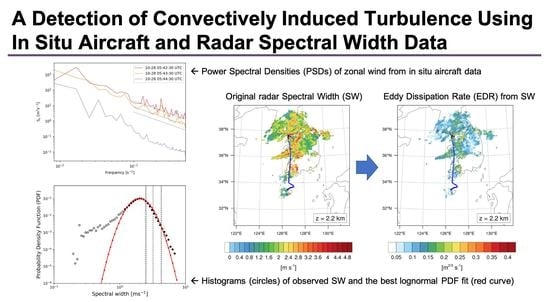
• 3D radar mosaic data showed shallow convective bands, which indicated high reflectivity in the lower part of the convective cloud and a high spectral width (SW) of more than 4 m s⁻¹ in the middle part. The high spectral width area coincided with the incident point in the horizontal and vertical directions.
• Using the simple statistical lognormal mapping technique (LMT) based on a lognormal distribution, SW was rescaled to EDR with more clear separations of high values and low values removed. The 0.3–0.35 EDR of SW near the turbulence spot is comparable to the 0.33–0.37 EDR from the aircraft data.
• Our numerical simulation used a WRF model with a 3 km resolution to simulate the convection system with time delay. Despite the systematic delay in the time, the model showed well-structured convective clouds, showing a similar intensity to radar reflectively.
• The strong turbulence appeared ahead (first) and along (second) the convection system, which were observed in the unresolved and resolved TKEs, respectively. The EDR scale of total TKE showed the comparable turbulence intensity (0.3–0.4 EDR), inferring the CIT occurrence near the incident location.
• For objective comparison in terms of the turbulence intensity, model-derived turbulence indicators were also remapped to EDR scale using the LMT and compared with the observation data, which included the absolute vertical velocity |w| and |w| divided by the Richardson number.
• Applying two diagnostic indices using the vertical velocity can provide a suitable indicator since high vertical velocity is common inside convection, which is one of the factors causing severe aviation incidents. Both diagnostics detected in-cloud CIT near the site. In |w|/Ri, however, turbulence intensity seemed to be too wide when the environment effect due to shear instability was considered.

References

1. Tvaryanas, A.P. Epidemiology of turbulence-related injuries in airline cabin crew, 1992–2001. Aviat. Space Environ. Med. 2003, 74, 970–976. [Google Scholar]
2. Sharman, R.; Lane, T. Aviation Turbulence; Springer International Publishing: Geneva, Switzerland, 2016; p. 523. [Google Scholar]
3. Kim, J.-H.; Sharman, R.; Strahan, M.; Scheck, J.W.; Bartholomew, C.; Cheung, J.C.H.; Buchanan, P.; Gait, N. Improvements in nonconvective aviation turbulence prediction for the world area forecast system. Bull. Am. Meteorol. Soc. 2018, 99, 2295–2311. [Google Scholar] [CrossRef] [Green Version]
4. Lester, P.F. Turbulence: A New Perspective for Pilots; Jeppesen Sanderson: Englewood, NJ, USA, 1994; p. 212. [Google Scholar]
5. Wolff, J.K.; Sharman, R.D. Climatology of upper-level turbulence over the contiguous United States. J. Appl. Meteorol. Clim. 2008, 47, 2198–2214. [Google Scholar] [CrossRef]
6. Kim, J.-H.; Chun, H.-Y. Statistics and possible sources of aviation turbulence over South Korea. J. Appl. Meteorol. Clim. 2011, 50, 311–324. [Google Scholar] [CrossRef]
7. Kim, S.-H.; Chun, H.-Y. Aviation turbulence encounters detected from aircraft observations: Spatiotemporal characteristics and application to Korean Aviation turbulence guidance. Meteorol. Appl. 2016, 23, 594–604. [Google Scholar] [CrossRef]
8. Ellrod, G.P.; Knapp, D.I. An objective clear-air turbulence forecasting technique: Verification and operational use. Weather. Forecast. 1992, 7, 150–165. [Google Scholar] [CrossRef] [Green Version]
9. Kim, J.-H.; Chun, H.-Y. A numerical study of clear-air turbulence (CAT) encounters over South Korea on 2 April 2007. J. Appl. Meteorol. Clim. 2010, 49, 2381–2403. [Google Scholar] [CrossRef]
10. Lee, D.-B.; Chun, H.-Y. A numerical study of aviation turbulence encountered on 13 February 2013 over the Yellow Sea between China and the Korean Peninsula. J. Appl. Meteorol. Clim. 2018, 57, 1043–1060. [Google Scholar] [CrossRef]
11. Knox, J.A. Possible mechanisms of clear-air turbulence in strongly anticyclonic flows. Mon. Weather. Rev. 1997, 125, 1251–1259. [Google Scholar] [CrossRef]
12. Knox, J.A.; McCann, D.W.; Williams, P.D. Application of the lighthill–ford theory of spontaneous imbalance to clear-air turbulence forecasting. J. Atmos. Sci. 2008, 65, 3292–3304. [Google Scholar] [CrossRef] [Green Version]
13. Kim, J.-H.; Chun, H.-Y.; Sharman, R.D.; Trier, S.B. The role of vertical shear on aviation turbulence within cirrus bands of a simulated western Pacific Cyclone. Mon. Weather. Rev. 2014, 142, 2794–2813. [Google Scholar] [CrossRef]
14. Lane, T.P.; Doyle, J.D.; Plougonven, R.; Shapiro, M.A.; Sharman, R.D. Observations and numerical simulations of inertia–gravity waves and shearing instabilities in the vicinity of a jet stream. J. Atmos. Sci. 2004, 61, 2692–2706. [Google Scholar] [CrossRef] [Green Version]
15. Koch, S.E.; Jamison, B.D.; Lu, C.; Smith, T.L.; Tollerud, E.I.; Girz, C.; Wang, N.; Lane, T.P.; Shapiro, M.A.; Parrish, D.D.; et al. Turbulence and gravity waves within an upper-level front. J. Atmos. Sci. 2005, 62, 3885–3908. [Google Scholar] [CrossRef]
16. Sharman, R.; Doyle, J.D.; Shapiro, M.A. An investigation of a commercial aircraft encounter with severe clear-air turbulence over Western Greenland. J. Appl. Meteorol. Clim. 2012, 51, 42–53. [Google Scholar] [CrossRef] [Green Version]
17. Lane, T.P.; Doyle, J.D.; Sharman, R.D.; Shapiro, M.A.; Watson, C.D. Statistics and dynamics of aircraft encounters of turbulence over Greenland. Mon. Weather. Rev. 2009, 137, 2687–2702. [Google Scholar] [CrossRef]
18. Elvidge, A.D.; Vosper, S.B.; Wells, H.; Cheung, J.C.H.; Derbyshire, S.H.; Turp, D. Moving towards a wave-resolved approach to forecasting mountain wave induced clear air turbulence. Meteorol. Appl. 2017, 24, 540–550. [Google Scholar] [CrossRef] [Green Version]
19. Grabowski, W.W.; Clark, T.L. Cloud–environment interface instability: Rising thermal calculations in two spatial dimensions. J. Atmos. Sci. 1991, 48, 527–546. [Google Scholar] [CrossRef]
20. Lane, T.P.; Sharman, R.D.; Clark, T.L.; Hsu, H.-M. An Investigation of turbulence generation mechanisms above deep convection. J. Atmos. Sci. 2003, 60, 1297–1321. [Google Scholar] [CrossRef]
21. Sharman, R.D.; Trier, S.B. Influences of gravity waves on convectively induced turbulence (CIT): A review. Pure Appl. Geophys. PAGEOPH 2018, 176, 1923–1958. [Google Scholar] [CrossRef]
22. Kim, J.-H.; Chun, H.-Y. A numerical simulation of convectively induced turbulence above deep convection. J. Appl. Meteorol. Clim. 2012, 51, 1180–1200. [Google Scholar] [CrossRef]
23. Lane, T.P.; Sharman, R.D.; Trier, S.B.; Fovell, R.G.; Williams, J.K. Recent Advances in the understanding of near-cloud turbulence. Bull. Am. Meteorol. Soc. 2012, 93, 499–515. [Google Scholar] [CrossRef] [Green Version]
24. Sharman, R.; Trier, S.B.; Lane, T.P.; Doyle, J.D. Sources and dynamics of turbulence in the upper troposphere and lower stratosphere: A review. Geophys. Res. Lett. 2012, 39. [Google Scholar] [CrossRef] [Green Version]
25. Trier, S.B.; Sharman, R.D.; Lane, T.P. Influences of moist convection on a cold-season outbreak of clear-air turbulence (CAT). Mon. Weather. Rev. 2012, 140, 2477–2496. [Google Scholar] [CrossRef]
26. Kim, S.-H.; Chun, H.-Y.; Sharman, R.D.; Trier, S.B. Development of near-cloud turbulence diagnostics based on a convective gravity wave drag parameterization. J. Appl. Meteorol. Clim. 2019, 58, 1725–1750. [Google Scholar] [CrossRef]
27. Sharman, R.D.; Pearson, J.M. Prediction of energy dissipation rates for aviation turbulence. Part I: Forecasting nonconvective turbulence. J. Appl. Meteorol. Clim. 2017, 56, 317–337. [Google Scholar] [CrossRef]
28. Pearson, J.M.; Sharman, R.D. Prediction of energy dissipation rates for aviation turbulence. Part II: Nowcasting convective and nonconvective turbulence. J. Appl. Meteorol. Clim. 2017, 56, 339–351. [Google Scholar] [CrossRef] [Green Version]
29. Gultepe, I.; Sharman, R.; Williams, P.D.; Zhou, B.; Ellrod, G.; Minnis, P.; Trier, S.; Griffin, S.; Yum, S.S.; Gharabaghi, B.; et al. A review of high impact weather for aviation meteorology. Pure Appl. Geophys. 2019, 176, 1869–1921. [Google Scholar] [CrossRef]
30. Sharman, R.; Tebaldi, C.; Wiener, G.; Wolff, J. An integrated approach to mid- and upper-level turbulence forecasting. Weather. Forecast. 2006, 21, 268–287. [Google Scholar] [CrossRef]
31. Kim, J.-H.; Chun, H.-Y. Development of the Korean Aviation Turbulence Guidance (KTG) System using the Operational Unified Model (UM) of the Korea Meteorological Administration (KMA) and Pilot Reports (PIREPs). J. Korean Soc. Aviat. Aeronaut. 2012, 20, 76–83. [Google Scholar] [CrossRef] [Green Version]
32. Lee, D.-B.; Chun, H.-Y. Development of the Global-Korean Aviation Turbulence Guidance (Global-KTG) System Using the Global Data Assimilation and Prediction System (GDAPS) of the Korea Meteorological Administration (KMA). Atmosphere 2018, 28, 223–232. (In Korean) [Google Scholar] [CrossRef]
33. Cho, J.Y.N.; Lindborg, E. Horizontal velocity structure functions in the upper troposphere and lower stratosphere: 1. Observations. J. Geophys. Res. Space Phys. 2001, 106, 10223–10232. [Google Scholar] [CrossRef]
34. Nastrom, G.D.; Gage, K.S. A climatology of atmospheric wavenumber spectra of wind and temperature observed by com-mercial aircraft. J. Atmos. Sci. 1985, 42, 950–960. [Google Scholar] [CrossRef] [Green Version]
35. International Civil Aviation Organization. Meteorological Service for International Air Navigation: Annex 3 to the Convention on International Civil Aviation, 14th ed.; ICAO International Standards and Recommended Practices: Montréal, QC, Canada, 2001; p. 128. [Google Scholar]
36. International Civil Aviation Organization. Meteorological Service for International Air Navigation: Annex 3 to the Convention on the International Civil Aviation, 17th ed.; ICAO International Standards and Recommended Practices: Montréal, QC, Canada, 2010; p. 206. [Google Scholar]
37. Kim, J.-H.; Chan, W.N.; Sridhar, B.; Sharman, R.D. Combined winds and turbulence prediction system for automated air-traffic management applications. J. Appl. Meteorol. Clim. 2015, 54, 766–784. [Google Scholar] [CrossRef] [Green Version]
38. Williams, J.K. Using random forests to diagnose aviation turbulence. Mach. Learn. 2014, 95, 51–70. [Google Scholar] [CrossRef] [Green Version]
39. Moninger, W.R.; Mamrosh, R.D.; Pauley, P.M. Automated meteorological reports from commercial aircraft. Bull. Am. Meteorol. Soc. 2003, 84, 203–216. [Google Scholar] [CrossRef] [Green Version]
40. Cornman, L.B.; Morse, C.S.; Cunning, G. Real-time estimation of atmospheric turbulence severity from in-situ aircraft meas-urements. J. Aircr. 1995, 32, 171–177. [Google Scholar] [CrossRef]
41. Sharman, R.D.; Cornman, L.B.; Meymaris, G.; Pearson, J.; Farrar, T. Description and Derived climatologies of automated in situ eddy-dissipation-rate reports of atmospheric turbulence. J. Appl. Meteorol. Clim. 2014, 53, 1416–1432. [Google Scholar] [CrossRef]
42. Cornman, L.B. Airborne In Situ Measurements of Turbulence; Springer International Publishing: Geneva, Switzerland, 2016; pp. 97–120. [Google Scholar]
43. Strauss, L.; Serafin, S.; Haimov, S.; Grubišić, V. Turbulence in breaking mountain waves and atmospheric rotors estimated from airborne in situ and Doppler radar measurements. Q. J. R. Meteorol. Soc. 2015, 141, 3207–3225. [Google Scholar] [CrossRef]
44. Champagne, F.H. The fine-scale structure of the turbulent velocity field. J. Fluid Mech. 1978, 86, 67–108. [Google Scholar] [CrossRef]
45. Piper, M.; Lundquist, J.K. Surface layer turbulence measurements during a frontal passage. J. Atmos. Sci. 2004, 61, 1768–1780. [Google Scholar] [CrossRef]
46. Kolmogorov, A.N. Dissipation of energy in the locally isotropic turbulence. Proc. R. Soc. Lond. Ser. A Math. Phys. Sci. 1991, 434, 15–17. [Google Scholar] [CrossRef]
47. Kolmogorov, A.N. The local structure of turbulence in incompressible viscous fluid for very large Reynolds numbers. Proc. R. Soc. Lond. Ser. A Math. Phys. Sci. 1991, 434, 9–13. [Google Scholar] [CrossRef]
48. Oncley, S.P.; Friehe, C.A.; Larue, J.C.; Businger, J.A.; Itsweire, E.C.; Chang, S.S. Surface-layer fluxes, profiles, and turbulence measurements over uniform terrain under near-neutral conditions. J. Atmos. Sci. 1996, 53, 1029–1044. [Google Scholar] [CrossRef] [Green Version]
49. Muñoz-Esparza, D.; Sharman, R.D.; Lundquist, J.K. Turbulence Dissipation rate in the atmospheric boundary layer: Observations and WRF mesoscale modeling during the XPIA field campaign. Mon. Weather. Rev. 2018, 146, 351–371. [Google Scholar] [CrossRef] [Green Version]
50. Ye, B.-Y.; Lee, G.; Park, H.-M. Identification and Removal of Non-Meteorological Echoes in Dual-Polarization Radar Data Based on a Fuzzy Logic Algorithm. Adv. Atmos. Sci. 2015, 32, 1217–1230. [Google Scholar] [CrossRef]
51. Muñoz-Esparza, D.; Sharman, R. An improved algorithm for low-level turbulence forecasting. J. Appl. Meteorol. Clim. 2018, 57, 1249–1263. [Google Scholar] [CrossRef]
52. Kim, S.-H.; Chun, H.-Y.; Kim, J.-H.; Sharman, R.D.; Strahan, M. Retrieval of eddy dissipation rate from derived equivalent vertical gust included in Aircraft Meteorological Data Relay (AMDAR). Atmos. Meas. Tech. 2020, 13, 1373–1385. [Google Scholar] [CrossRef] [Green Version]
53. Skamarock, W.; Klemp, J.B.; Dudhia, J.; Gill, D.O.; Barker, D.; Duda, D.M.; Huang, X.; Wang, W.; Powers, J.G. A Description of the Advanced Research WRF Version 3. NCAR Techical Note NCAR/TN475+STR; University Corporation for Atmospheric Research: Boulder, CO, USA, 2008; p. 113. [Google Scholar]
54. Trier, S.B.; Sharman, R.D. Convection-permitting simulations of the environment supporting widespread turbulence within the upper-level outflow of a mesoscale convective system. Mon. Weather. Rev. 2009, 137, 1972–1990. [Google Scholar] [CrossRef] [Green Version]
55. Trier, S.B.; Sharman, R.D. Mechanisms influencing cirrus banding and aviation turbulence near a convectively enhanced upper-level jet stream. Mon. Weather. Rev. 2016, 144, 3003–3027. [Google Scholar] [CrossRef]
56. Thompson, G.; Field, P.R.; Rasmussen, R.M.; Hall, W.D. Explicit Forecasts of winter precipitation using an improved bulk microphysics scheme. Part II: Implementation of a new snow parameterization. Mon. Weather. Rev. 2008, 136, 5095–5115. [Google Scholar] [CrossRef]
57. Nakanishi, M.; Niino, H. An improved mellor–yamada level-3 model: Its numerical stability and application to a regional prediction of advection fog. Bound. Layer Meteorol. 2006, 119, 397–407. [Google Scholar] [CrossRef]
58. Iacono, M.J.; Delamere, J.S.; Mlawer, E.J.; Shephard, M.W.; Clough, S.A.; Collins, W.D. Radiative forcing by long-lived greenhouse gases: Calculations with the AER radiative transfer models. J. Geophys. Res. Space Phys. 2008, 113, D13103. [Google Scholar] [CrossRef]
59. Ek, M.B.; Mitchell, K.E.; Lin, Y.; Rogers, E.; Grunmann, P.; Koren, V.; Gayno, G.; Tarpley, J.D. Implementation of Noah land surface model advances in the National Centers for environmental prediction operational mesoscale Eta model. J. Geophys. Res. Space Phys. 2003, 108, 8851. [Google Scholar] [CrossRef]
60. Kain, J.S. The kain–fritsch convective parameterization: An update. J. Appl. Meteorol 2004, 43, 170–181. [Google Scholar] [CrossRef] [Green Version]
61. Park, S.; Kim, J.; Sharman, R.D.; Klemp, J.B. Update of upper level turbulence forecast by reducing unphysical components of topography in the numerical weather prediction model. Geophys. Res. Lett. 2016, 43, 7718–7724. [Google Scholar] [CrossRef]
62. Park, S.-H.; Klemp, J.B.; Kim, J.-H. Hybrid mass coordinate in WRF-ARW and Its impact on upper-level turbulence forecasting. Mon. Weather. Rev. 2019, 147, 971–985. [Google Scholar] [CrossRef]
63. Kim, J.-H.; Sharman, R.D.; Benjamin, S.G.; Brown, J.M.; Park, S.-H.; Klemp, J.B.; Benjamin, S.; Klemp, J. Improvement of mountain-wave turbulence forecasts in NOAA’s Rapid refresh (RAP) model with the hybrid vertical coordinate system. Weather. Forecast. 2019, 34, 773–780. [Google Scholar] [CrossRef]
64. Beck, J.; Brown, J.; Dudhia, J.; Gill, D.; Hertneky, T.; Klemp, J.; Wang, W.; Williams, C.; Hu, M.; James, E.; et al. An evaluation of a hybrid, terrain-following vertical coordinate in the WRF-based RAP and HRRR models. Weather. Forecast. 2020, 35, 1081–1096. [Google Scholar] [CrossRef] [Green Version]
65. Gultepe, I.; Starr, D.O. Dynamical structure and turbulence in cirrus clouds: Aircraft observations during fire. J. Atmos. Sci. 1995, 52, 4159–4182. [Google Scholar] [CrossRef] [Green Version]
Figure 1. The flight route (solid line) between Gimpo (Seoul) and Jeju Island, South Korea, and the observed location of the plane (red dot) at 05:42 UTC on 28 October 2018.
Remotesensing 13 00726 g001
Figure 2. (a) Time series of the vertical acceleration (blue), wind speed (red), and wind direction (green) with the time of the turbulence incident (yellow) and (b) time series of the flight altitude (red) and vertical acceleration (blue) during 05:26–06:38 UTC on 28 October 2018.
Remotesensing 13 00726 g002aRemotesensing 13 00726 g002b
Figure 3. The scatter density plots of correlation for (a) u-, (b) v-wind components, and (c) wind speed between the quick access recorder (QAR) data and the fifth generation of the European Centre for Medium-range Weather Forecast reanalysis (ERA5) data during the research period from 05:40 UTC to 06:30 UTC on 28 October 2018. Color scales are probability of occurrence (%), and the black diagonal lines are the perfect correlation. Mean absolute error (MAE) and root mean square error (RMSE) values are also depicted in each plot.
Remotesensing 13 00726 g003
Figure 4. The power spectral densities (PSDs) of the zonal wind calculated from the quick access recorder (QAR) data at 05:42:30, 05:43:30, and 05:44:30 UTC on 28 October 2018. Dotted black lines indicate the k−5/3 slope of the eddy dissipation rate (EDR) values matching 0.15, 0.22, and 0.34 m2/3 s−1 (bottom to top), which correspond to the light (LGT), moderate (MOD), and severe (SEV) turbulence, respectively, for medium-size aircraft [3,28,38,42].
Remotesensing 13 00726 g004
Figure 5. (Left) Horizontal radar reflectivity and (right) spectral width (SW; right) at altitudes of (top) 2.2 and (bottom) 4.8 km at 05:40 UTC 28 October 2018. The location of the turbulence encounter is depicted as a black asterisk and the flight routes are indicated as a dotted line according to the observed in situ EDR values (blue: NIL, green: LGT, yellow: MOD, and pink: SEV, based on [3,27,37,41]).
Remotesensing 13 00726 g005
Figure 6. (Left) Latitude–altitude cross-sections of radar reflectivity and (right) SW centered on the longitude of Table 126.64°E at 05:40 UTC on 28 October 2018. Bottom panels are magnifications of the accident region of the latitude of 37–38°N. The location of the turbulence encounter is indicated by the black asterisk, and waypoints along the flight route are indicated by the colored dots according to the EDR values (blue: NIL, green: LGT, yellow: MOD, and pink: SEV).
Remotesensing 13 00726 g006
Figure 7. Histograms (circles) of the observed radar SW data below z = 8 km from 04:50 to 05:50 UTC on 28 October 2018 and the best lognormal probability density function (PDF) fit (red curve) in the log-log domain. Filled circles indicate the data used for constructing the best PDF fit, while open circles are excluded for calculating the best fit. The vertical black dashed lines represent the thresholds of the SW for the LGT, MOD, and SEV turbulence (left to right), corresponding to EDR values of 0.15, 0.22, and 0.34 m2/3 s−1, respectively.
Remotesensing 13 00726 g007
Figure 8. (Left) Original radar SW data and (right) SW-derived EDR at an altitude of 2.2 km at 05:40 UTC on 28 October 2018. The location of the turbulence encounter is depicted as an asterisk, and the flight routes are indicated as colored dotted lines according to the in situ EDR values (blue: NIL, green: LGT, yellow: MOD, and pink: SEV).
Remotesensing 13 00726 g008
Figure 9. Latitude–altitude cross-sections of (left) original SW and (right) SW-derived EDR centered on the longitude of Table 126. 64°E) at 05:40 UTC on 28 October 2018. Bottom panels are magnifications of the incident region at 37°–38°N. The location where the turbulence was encountered is indicated as an asterisk, and the flight routes are indicated as colored dots according to the in situ EDR values (blue: NIL, green: LGT, yellow: MOD, and pink: SEV).
Remotesensing 13 00726 g009
Figure 10. Locations of model domains 1 and 2, which have 9 and 3 km horizontal grid spacing, respectively.
Remotesensing 13 00726 g010
Figure 11. Zonal wind energy spectra with different lead times at a height of 2 km at 00:00 UTC 28 October 2018. Each spectrum corresponding to 0, 3, 6, and 12 h forecasts was calculated over domain 2 in the zonal direction and was averaged in the meridional direction.
Remotesensing 13 00726 g011
Figure 12. (Upper panels) Simulated column-maximum radar reflectivity at (left) 05:40 UTC and (right) 06:40 UTC on 28 October 2018 obtained from domain 2. (Lower panels) Latitude–altitude cross-sections of simulated radar reflectivity between 126° and 127°E at 06:40 UTC on 28 October 2018 for (left) entire latitude range of domain 2 and (right) magnified region. The location where the turbulence was encountered is indicated by the asterisk and the flight routes are indicated as dotted lines according to the EDR estimates (blue: NIL, green: LGT, yellow: MOD, and pink: SEV).
Remotesensing 13 00726 g012
Figure 13. Horizontal distributions of (upper panels) turbulent kinetic energy (TKE) and (lower panels) EDRs converted from (left) sub-grid scale (SGS), (middle) resolved, and (right) total TKEs at 06:40 UTC on 28 October 2018 at the altitude of 2.2 km. The asterisk indicates the location of the CIT event.
Remotesensing 13 00726 g013
Figure 14. As in Figure 7, except for the PDFs of the absolute vertical velocity |w| (left) and |w| divided by the Richardson number (|w|/Ri). The PDFs were calculated from a 1 h model output of 28 October 2018. The coefficients of the best fit curve are indicated in the upper left side.
Remotesensing 13 00726 g014
Figure 15. Horizontal distribution of the EDR converted from (left) the absolute value of vertical velocity |w| and (right) |w|/Ri at 06:40 UTC on 28 October 2018 at z = 2.2 km. The asterisk indicates the location of the CIT event.
Remotesensing 13 00726 g015