Passive Remote Sensing of Ice Cloud Properties at Terahertz Wavelengths Based on Genetic Algorithm

Abstract

Ice clouds play a critical role in the balance of the earth–atmosphere radiation system, but there are some limitations in the existing remote sensing methods for ice clouds. Terahertz wave is expected to be the best waveband for retrieving ice clouds, with terahertz wavelengths in the order of the size of typical ice cloud particles. An inversion method for the remote sensing of ice clouds at terahertz wavelengths based on genetic algorithm is proposed in this paper. First, suitable channel sets in the terahertz band, which are mainly a combination of absorption lines and window regions, are determined. Then, to improve the efficiency of the generation of the retrieval database, based on the brightness temperature simulated by the atmospheric radiative transfer simulator (ARTS) for different cloud parameters, a fast forward operator is constructed using three-dimensional interpolation to simulate the brightness temperature difference between clear sky and a cloudy scene. Finally, an inversion model to retrieve the ice cloud base height, the effective particle diameter and the ice water path is established based on the genetic algorithm, and an analysis of the inversion errors is performed. The results show that the forward operator, constructed by the nearest interpolation, can accurately calculate the brightness temperature difference at a high speed. The proposed inversion method at terahertz wavelengths based on the genetic algorithm can achieve the expected scientific requirement. The absolute error of the cloud height is around 0.2 km, and the absolute error of the low ice water path (below 20 g/m²) is small, while the relative error of the high ice water path is generally maintained at around 10%, and the absolute error of the effective particle diameter is mostly around 4 μm.

1. Introduction

Ice clouds play a key role in regulating the radiant energy flow in the earth–atmosphere radiation budget through scattering and absorption processes [1]. The physical characteristics of ice clouds are important parameters in climate and weather forecast models—for instance, cloud height, particle size and ice water path [2,3]. However, the current remote sensing of ice cloud parameters is insufficient, leading to considerable uncertainties in numerical weather prediction (NWP) and climate models, where accurate presentation of ice clouds is needed to optimize the assimilation [4,5]. The effective detection of ice clouds will greatly facilitate global and local climate research, improve the accuracy of numerical weather forecasts and provide services for extreme weather warning, weather modification and aviation meteorology [6].

The present methods to retrieve ice cloud parameters mainly include passive and active sensors, which have advanced our knowledge of ice clouds, but there is still a large degree of uncertainty in the measurements. For visible and infrared passive remote sensing, the absorption of ice clouds in this waveband is critical and thus the penetrability is low for thick clouds [7]. As a result, the retrieval only represents the characteristics of the upper layer clouds or thin cirrus clouds [8,9]. Although passive remote sensing in microwave bands displays better penetration for thick clouds, the channel frequencies in the existing sensors are generally no more than 190 GHz and relatively sensitive to large ice particles [10]. Active remote sensing is more suitable for retrieving the whole ice cloud depth with an admirable resolution, but it only samples the atmosphere just below the satellite, so it has limited spatial coverage. Holl et al. stated that the joint inversion by lidar and radar can achieve greater retrieval accuracy compared with passive remote sensing methods [11]. However, the wavelengths applied in the existing active sensing instruments are primarily sensitive to relatively large particle or small particle portions, hindering the collection of comprehensive cloud information. To overcome the limitations of the existing active sensors (lidar and millimeter-wave radars) and passive sensors (visible, infrared and microwave radiometers), many scholars have proposed the application of passive remote sensing of ice cloud characteristics at terahertz wavelengths (0.1–10 THz, 30 μm–3 mm) [12,13,14,15]. Owing to the comparable order of ice particle sizes and the wavelengths, the terahertz wave is expected to be able to scan the entire ice particle size range and obtain comprehensive information about ice clouds.

Considering the potential to retrieve the properties of ice clouds, research institutions in many countries have proposed corresponding plans to explore the technology of spaceborne terahertz instruments in succession. The inversion of ice clouds at terahertz wavelengths is essentially a pathological problem, and some inversion algorithms have been put forward in the existing measurements. Evans et al. proposed the Bayesian Monte Carlo integration (BMCI) method and stated the procedure and performance by simulated scenes [16]. Further, the method was applied to retrieve the ice water path and particle sizes from observations during the Cirrus Regional Study of Tropical Anvils and Cirrus Layers (CRYSTAL) Florida Area Cirrus Experiment (FACE) campaign [17]. Jiménez et al. proposed a neural network (NN) method [18] and tested the retrieval accuracy of the cloud height, ice water path and ice particle size using the Colorado training dataset and the Chalmers training dataset [12]. However, both the inversion algorithms required the creation of a perfect and practical retrieval database that contained a large number of measured local atmospheric profiles and the corresponding simulated brightness temperature. The retrieval accuracy depends on the amount of available information in the database to a large extent, which is more complicated and time-consuming. Other methods have also been tested, such as the optimal estimation [19] and Markov chain Monte Carlo [20], which were quickly discarded, as the nonlinearity of the inversion problem implies a costly recalculation of the weighting functions.

Focusing on the remote sensing technology at terahertz wavelengths, we demonstrated its feasibility in ice cloud detection and introduced an inversion method based on multiple lookup tables. The characteristic parameters of brightness temperature difference and brightness temperature difference slope were derived to quantify the effects of the ice water path and particle size on the zenith radiation spectrum. A weighted least square fit that matched the modeled parameters was proposed to retrieve ice clouds’ microphysical parameters [21,22,23]. However, the establishment of the multiple lookup tables requires a high standard in the selection of different channels and characteristic parameters. Recently, a multi-channel regression inversion algorithm to remotely sense the ice water path passively was presented, which was faster and simpler. Combinations of different channels were selected to eliminate the effects of other related factors (i.e., ice cloud height and ice particle size), in order to realize the inversion of the ice water path directly [24]. In fact, the inversion of ice clouds at terahertz wavelengths can eventually be simplified to a global optimization problem, which is achieving the optimal value of the independent variables when the objective function (the difference between the observation and simulation) is optimal. Intelligent algorithms have the ability to search globally, which is suitable for solving problems of this type, especially the genetic algorithm, tabu search, particle swarm optimization and immune algorithm. All of the optimization algorithms are simulations of natural processes and have the unique advantage of providing a global optimal solution to the problem, after continuous improvement by predecessors.

The goal of this work is to introduce a new inversion method on the basis of the genetic algorithm to retrieve the ice cloud microphysical parameters (the effective particle diameters and ice water paths) at terahertz wavelengths. The main structure of this article is as follows: first, the basic principles of the passive remote sensing of ice cloud parameters at terahertz wavelengths are introduced. Then, concerning the steps of the research process, the inversion method based on the intelligent genetic algorithm is discussed in detail. Finally, the inversion errors are analyzed using the actual simulation data, and the effectiveness of the proposed method is validated.

2. Basic Principles

2.1. Process of Ice Cloud Inversion at Terahertz

The values of the nadir brightness temperatures received by the terahertz radiometers are affected by ice clouds. Since the emission ability of the ice crystals in the terahertz band is relatively weak, the scattering process plays a crucial role in radiative transfer. Therefore, the terahertz radiation emitted upward from the lower warmer atmosphere (usually the water vapor in the lower troposphere) will be strongly scattered by ice clouds [25]. The attenuation of the brightness temperature at different frequencies depends on the characteristics of ice clouds. Thus, a direct relationship can be established between the reduction of the brightness temperature and the ice cloud parameters.

As shown in Figure 1, the inversion of the ice cloud parameters at the terahertz waveband has three aspects: first, the terahertz radiometer detects the brightness temperature at different frequencies; second, the forward radiative transfer model is used to simulate the brightness temperature of the corresponding channels; and third, the appropriate inversion method is used to obtain the ice cloud parameters.

To avoid the influence of by atmospheric profiles, we used the brightness temperature differences as the observed characteristic values (i.e., the values of the brightness temperature under a clear sky minus the values of the brightness temperature under a cloudy scene). The inversion method was applied to determine the ice cloud parameters by which the simulated brightness temperature difference was closest to the detected values. In other words, the inversion process can be converted to ascertain the variables of the ice cloud parameters $\widehat{x}$, which allows the objective function $f\left(\widehat{x}\right)$ to reach its minimum, shown as follows:

$$f\left(x\right)={\displaystyle \sum }_{i=1}^m\left|R_i\left(x\right)-I_i\left(x\right)\right|$$

(1)

where x denotes the ice cloud parameters, i.e., cloud height H, ice water path (IWP) and effective particle diameter D. In general, the optical thickness of the ice clouds would increase with the increase in IWP and D, which will also lead to an increase in the brightness temperature difference between the cloudy scene and clear sky before the saturation limit [26]. Moreover, m is the number of channels. The detected brightness temperature difference of the ith channel is R_i(x). The simulated brightness temperature difference of the ith channel is I_i(x). Equation (1) shows that the closer the objective function f(x) is to 0, the more optimized the value of x is.

2.2. Selection of Channel Sets

The terahertz radiometer passively receives the external energy of terahertz radiation, and therefore, selecting the appropriate frequency channel sets is the first step to retrieve the properties of ice clouds. The channels of the actual radiometer are passbands with certain widths. Moreover, even for the same center frequency, it usually has several different offsets. The main objective in selecting a frequency channel is to avoid the influence of irrelevant factors and improve the sensitivity to ice cloud parameters, where the macroscopic physical parameters of ice clouds include the cloud height, and the microphysical parameters include the ice water path and particle size.

The absorption line of the spectrum should be selected as the center frequency, in order to reduce the effects of the characteristics of the surface and lower atmosphere on the nadir spectrum. The properties of ice clouds at different levels can be acquired at a lower cost by setting the offsets along the center frequency. The larger the absorption coefficient, the greater the height of weight function peaks, and the greater the height of the effective emission layer of the terahertz radiation. Therefore, the ice clouds will only have an attenuation effect above the effective layer height. Because of the weak penetrability into deep clouds, the high-frequency channels are usually sensitive to ice clouds at the upper layer, whereas the low-frequency channel is sensitive to the low-level ice clouds. For different offsets at the same center frequency, the channel with the smaller offset is more sensitive to higher clouds because it is closer to the absorption line and has a higher opacity. Simultaneously, a significant difference exists between a clear sky and a cloudy sky in terms of the window channels. Therefore, the information about the ice clouds acquired by the window channels is significantly different from that obtained from the absorption lines.

The terahertz radiometer has important benefits for the next generation of meteorological satellites. Combined with the current research—for example, the Compact Scanning Submillimeter-wave Imaging Radiometer (CoSSIR) [17,25], the International Sub-Millimeter wave Airborne Radiometer (ISMAR) [27] and Ice Cloud Imager (ICI) [28]—channel sets in the terahertz band were selected comprehensively, as shown in

Table 1. Information on the channels in the terahertz band.

Center Frequency (GHz)	Center Wavelength (μm)	Frequency Offset (GHz)	Channel Characteristics
118.75	2526.3	±1.1, ±1.5, ±2.1, ±3.0, ±5.0	oxygen
157.05	1910.2	±2.6	window
183.31	1636.6	±1.0, ± 3.0, ±7.0	water vapor
243.20	1233.6	±2.5	window
325.15	922.7	±1.5, ±3.5, ±9.5	water vapor
424.70	706.3	±1.0, ±1.5, ±4.0	oxygen
448.0	669.6	±1.4, ±3.0, ±7.2	water vapor
664.0	451.8	±4.2	window
874.4	343.1	±6.0	window

.

3. Method for Ice Cloud Inversion

3.1. Forward Radiative Transfer Model

The atmospheric transmission of terahertz radiation is performed using the atmospheric radiative transfer simulator (ARTS). ARTS is a highly modular, expandable and universally applicable software that can be used to simulate and calculate the process of atmospheric radiative transmission from microwaves to thermal infrared waves [29,30].

The forward radiative transfer model uses a line-by-line integral method for the attenuation caused by the absorption of gas molecules and can solve the line absorption problems of overlapping absorption bands and non-uniform atmospheric paths. Simultaneously, the calculation of the absorption caused by the Zeeman effect and molecular collision is added. In the simulation, the profiles of the temperature, relative humidity, pressure and trace gas compositions, as inputs of the model, are drawn from the Fast Atmospheric Signature Code (FASCOD) standard database [31]. The spectroscopic parameters of molecular absorption are drawn from the HITRAN2012 database, created by the U.S. Air Force Cambridge Research Laboratory [32].

ARTS treats the scattering attenuation of particles, such as clouds and aerosols, precisely. For the calculation of the single scattering properties of ice particles, ARTS applies the Mie scattering theory or the T matrix method. For particle ensembles, particle size distribution models are provided, such as the mono-disperse particle distribution, gamma distribution, log-normal distribution and McFarquhar and Heymsfield (MH) model. Then, the discrete ordinate iterative (DOIT) method is used to address one-dimensional (1D) particle scattering, and the Monte Carlo (MC) method is used to manage three-dimensional (3D) particle scattering and multiple scattering problems. Geer et al. calculated the scattering properties of ice cloud and snow particles of different shapes and compared them with the measured data. It was demonstrated that the ice cloud particles were typically smaller than the snow particles and hence were less effective scatterers, and the choice of the particle shape was less important for ice clouds in the terahertz band [33]. Therefore, similar to the hypothesis given in the research of Evans et al., Brath et al. and Liu et al. [16,17,34,35], the single scattering properties of ice cloud particles were calculated using the Mie theory [36]. The Mie theory plays an important role in light scattering of electromagnetic wave by homogeneous spherical particles, in which the scattered field is represented as an infinite series of fields of spherical multipoles [37]. The gamma distribution was applied to describe the scale characteristics of particle ensembles, as follows:

$$N\left(D\right)=N_0{D}^{\mu }{e}^{-\lambda D}$$

(2)

where N(D) is the number density of the ice particles corresponding to D, N₀ is the intercept of the gamma distribution, μ identifies the spread of the distribution, and λ is the slope of the distribution, which is dependent on the dispersion and D.

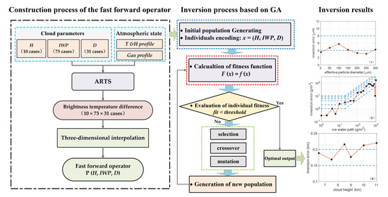
3.2. Construction of Fast Forward Operator

In the process of searching for the optimal solutions of the objective function f(x), it is necessary to repeatedly calculate the simulated brightness temperature differences in each iterative step to match the situation that is closest to the detected brightness temperature differences. Therefore, on the basis of fast-radiative transfer models, such as the Community Radiative Transfer Model (CRTM) and Radiative Transfer for TOVS (RTTOV), a fast forward operator was constructed by combining database and interpolation to simulate the brightness temperature differences efficiently.

Figure 2 depicts a basic flowchart for the construction of the fast forward operator. First, different ice cloud scenes were selected for simulations. Specifically, a total of 10 cases of cloud heights were selected, which were 6.5, 7.0, 7.5, 8.0, 8.5, 9, 9.5, 10, 10.5 and 11 km, respectively. The low ice water paths were dense, 1–20 g/m² for every 1 g/m², and the high ice water paths had a relatively low density of 20–100 g/m², taken for every 10 g/m², and 100–1000 g/m², taken for every 20 g/m², for a total of 73 cases. The values of the effective particle diameters were 2 μm and 10–300 μm for every 10 μm, for a total of 31 cases. Then, ARTS was applied to simulate the nadir brightness temperature of different channels in 10 × 73 × 31 = 22,630 combined ice cloud scenes. Simultaneously, the nadir brightness temperatures in the clear sky scenes were also simulated. Thus, a total of 22,630 cases of brightness temperature differences of different channels could be calculated. Thirdly, 3D interpolation was used to construct the forward operator P (H, IWP, D), as shown in (2). When inputting the H, the IWP and the D, the corresponding brightness temperature difference I (H, IWP, D) of different channels can be quickly obtained.

I (H, IWP, D) = P (H, IWP, D)

(3)

3.3. Inversion Method Based on the Genetic Algorithm

The genetic algorithm (GA) is a metaheuristic algorithm inspired by the process of natural selection. It was first proposed by Holland [38] in 1975 and was then summarized by DeJong and Goldberg et al. [39,40]. The GA is commonly used to generate high-quality solutions to optimization and search problems. The principle of GA is based on the concept of Darwin’s theory of evolution. It encodes the parameters of the problem into chromosomes and then uses iterative methods to select, cross and mutate the genes to allow for the exchange of this information within a population. Generally, the algorithm comes to an end when either the maximum number of iterations has been reached or the satisfactory fitness of the population has been satisfied. A chromosome that meets the optimization goal is finally generated. The processes of the GA can be divided into three steps: initialization, fitness scaling and genetic operations. Figure 3 depicts a basic flowchart of the intelligent inversion of ice cloud parameters based on the GA and each step is defined in detail below.

• Step 1: Initialization (Including Individual Encoding and Generation of Initial Population)

Since the GA cannot directly deal with the ice cloud parameters of the problem space, it is necessary to determine a feasible solution to the problems of the chromosomes or individuals in the genetic space by coding. The double vector encoding method was adopted here, for the GA could be directly performed on the phenotype of the solution. There were three ice cloud parameters in the optimal solutions, i.e., x = (H, IWP, D); thus, three chromosomes composed of three vectors were constructed in which the values on each gene corresponded to the possible solutions. The population size was set to 200, and the maximum generation was set to 1000. Other relevant settings for the initial population were generated through the creation function by default. Generally, the larger the population size was and the more the evolutionary generations iterated, the better the optimal individual $\widehat{x}$ fit for function value $f\left(\widehat{x}\right)$, but the iteration time is longer.

• Step 2: Fitness Scaling

The fitness function is a criterion for distinguishing the quality of individuals in the population. It is usually transformed by the objective function. Here, we needed to find the minimum value of the objective function f(x), so the objective function (i.e., Equation (1)) was taken as the fitness function F(x) directly, i.e., F(x) = f(x). The smaller the fitness function value was, the more optimized solution of the ice cloud parameters could be obtained. As to the fitness scaling method, the rank function was applied.

• Step 3: Genetic Operations (Including Selection, Crossover and Mutation)

Good individuals are selected from the old population as parents with a certain probability to generate a new population. The probabilities of being selected for the ice cloud parameters were related to the fitness values, and parameters with large fitness values were eliminated. The stochastic uniform method was applied as the selection method. To ensure convergence, the GA adopts the elite retention strategy; that is, the elite parameters in the parents will pass directly to the children without any crossover or mutation. Here, the elite count was set to 0.05 times the population size by default. The cross fraction indicated the proportion of individuals in the children generated by the crossover to the number of non-elite individuals in the parents, which was set to 0.8 here. The crossover was the most important genetic operation in the GA, resulting a new excellent individual. Mutation made small random changes to the ice cloud parameters related to the current optimal solution to produce better results. According to different types of constraints, different mutation functions were provided, such as Gaussian, uniform and adaptive feasible.

The upper and lower limits of the ice cloud parameters were set in this algorithm, where the range of the cloud height H was 6.5 to 11 km, the range of the ice water path IWP was 1 to 1000 g/m², and the range of the effective particle diameter D was 2 to 300 μm, respectively. To maintain relative consistency in the numerical values for the three parameters during the search, they were first subjected to the dimensionless operation. The H, IWP and D were treated as follows: (H – 6.5 km)/1 km, log10 (IWP/1 g/m²) and D/100 μm, and the corresponding dimensionless bounds became 0–4.5, 0–3 and 0.02–3, respectively. The GA could open parallel calculations to save time while calculating the fitness value of each ice cloud parameter.

4. Application of the Method and Results

4.1. Verification of the Fast Forward Operator

Based on the 22,630 cases of the nadir brightness temperature differences in the different channels, the construction of a fast forward operator by 3D interpolation was proposed. To further verify the accuracy of the forward operator, five different cloud heights between 6.5 and 11 km, five different ice water paths between 1 and 1000 g/m² and five different effective particle diameters between 2 and 300 μm were selected. Then, the nadir brightness temperature differences of the 21 channels in 5 × 5 × 5 = 125 combined ice cloud scenes were simulated. For the 22,630 pre-calculated nadir temperature differences, the nearest, linear and spline 3D interpolation methods were applied to obtain the brightness temperature difference of the 21 channels in the 125 cases.

Figure 4 depicts the scatter plots of the brightness temperature differences simulated and the three interpolated brightness temperature differences, with a critical relative error in interpolation boundary of 20% compared with the simulations. The nearest interpolation method was the best of the three methods, and the proportion of the points within the 20% relative error was 81.2%, whereas the proportions of the linear interpolation and spline interpolation were 64.0% and 59.2%, respectively. In addition, the inversion test showed that the nearest interpolation was more efficient than the other two methods.

4.2. Ice Cloud Inversion Error Analysis

For the sake of verifying the effectiveness of the inversion algorithm based on GA, an ice cloud scene with altitude of 8.5 km, IWP of 400 g/m² and effective particle diameter of 200 μm was chosen for a case study. The variation in the fitness function value during the inversion search is shown in Figure 5, where the abscissa is the evolutionary generation and the ordinate is the fitness function value, including the mean fitness function value of the population and the best fitness function value of the optimal individuals. Figure 5a,b are the curves of the fitness function value, where the coordinates are taken on a normal scale and logarithmic scale, respectively. The figures show that in the early stage of evolution, when the individual was far from the ideal value, the optimal solution rapidly improved. In the later stage of evolution, the population evolved slowly and it stagnated when the population evolved to 20 generations. With further increases in generations, the fitness function values of the optimal individual found by the GA was continuously reduced to around 0, and the algorithm stopped at around 55 generations. The ice cloud height, ice water path and effective particle diameter obtained at this time were 8.4984 km, 402.2138 g/m² and 196.3625 μm, respectively, indicating that the genetic algorithm is not limited by the local optimal solution and can effectively find the optimal solution.

The results of the inversion were quantitatively evaluated by comparing the retrieved values with the true values of the ice cloud parameters. In the inversion case, the values of the cloud heights were 6.5, 7.5, 8.5, 9, 10 and 11 km; the values of the ice water paths were 1, 2, 4, 6, 10, 20, 40, 60, 100, 150, 200, 300, 400, 500, 600, 700, 800, 900 and 1000 g/m²; and the values of the effective particle diameters were 2, 50, 100, 150, 200, 250 and 300 μm. The brightness temperature, simulated by ARTS for each case, was input into the GA for inversion. To avoid the influence of outliers, the median error was applied to replace the standard deviation, since it was more robust against rare outliers than the root mean square error (RMSE) [15]. The H and D were evaluated by the median absolute error (MAE). The IWP value had a large dynamic range. Therefore, for the evaluation of low IWP values, we used the MAE, and for the high IWP values, we used the median relative error (MRE) [12]; that is,

$$\mathrm{MAE}=median\left(\left|{\widehat{x}}_i-x_i\right|\right)$$

(4)

$$\mathrm{RE}=median\left(\frac{\left|{\widehat{x}}_i-x_i\right|}{x_i}\times 100\%\right)$$

(5)

where ${\widehat{x}}_i$ is the ith value of the retrieved ice cloud parameters and $x_i$ is the ith true value.

Figure 6 shows the retrieval performance based on the GA for the different ice cloud parameters. Figure 6a displays the MAEs for the different cloud heights. Figure 6b presents the median error for the different ice water paths. The MAEs of 1, 2, 4, 6, 8 and 10 g/m² are marked with dashed lines for the low ice water path below 20 g/m², and the MREs of 5%, 10%, 20%, 30%, 40% and 50% are marked with dashed lines for the high ice water path above 20 g/m². Figure 6c demonstrates the MAEs for the different effective particle diameters. The absolute errors for the cloud height remained at around 0.2 km, with a minimum value of 0.1686 km. The absolute errors of the low ice water path, which were below 20 g/m², remained within 3 g/m². Moreover, the relative errors for the high ice water paths were generally maintained at around 10%, with a maximum value of 18.3627%. The absolute errors of the effective particle diameters were mostly maintained at around 4 μm and the maximum was 4.7075 μm when the diameter was 100 μm.

5. Discussion and Summary

In this study, we applied the genetic algorithm to the inversion of ice cloud properties at terahertz wavelengths. First, suitable channel sets in the terahertz band are determined, which are mainly a combination of absorption lines and window regions. Then, a fast forward operator is constructed using three-dimensional interpolation to simulate the brightness temperature difference between clear sky and a cloudy scene. Finally, an inversion model to retrieve the ice cloud base height, the effective particle diameter and the ice water path is established based on the genetic algorithm, and an analysis of the inversion errors is performed.

The results show that the forward operator, constructed by the nearest interpolation, can accurately calculate the brightness temperature difference at a high speed. The proposed inversion method at terahertz wavelengths based on the genetic algorithm can achieve the expected scientific requirement. The absolute error of the cloud height is around 0.2 km, and the absolute error of the low ice water path (below 20 g/m²) is small, while the relative error of the high ice water path is generally maintained at around 10%, and the absolute error of the effective particle diameter is mostly around 4 μm.

Buehler et al. proposed a formal scientific mission requirement for a passive submillimeter-wave cloud ice mission based on the current background and early research [15], such as that of Jiménez and Evans [16,18], in which the accuracy index of the inversion errors was formulated. The requirements are as follows: the cloud height should be less than 500 m, the low ice water path should be less than 10 g/m², the high ice water path should be less than 50%, and the particle diameter should be less than 50 μm. Therefore, the inversion of the ice cloud parameters based on the GA can achieve the expected scientific requirement.

The research results may provide theoretical support and a reference for the development of new generation of ice cloud detection loads. However, inversion technology for the passive remote sensing of ice clouds at terahertz based on the genetic algorithm is expected to be further developed in the future. First, the simulation in this paper was theoretically conducted with several factors simplified into ideal conditions for convenience. For instance, the ice cloud was supposed to be homogeneous in the simulation, which affected the retrieval accuracy to some extent. Second, to improve the accuracy, the density of the selected values in the simulation can be increased while constructing the fast forward operator after three-dimensional interpolation. Third, the actual ice water path and particle size satisfy certain constraints, so the constrained solution in the genetic algorithm not only sets the upper and lower limit boundaries but also can be combined with physical information concerning the actual ice clouds, such as linear or nonlinear constraints.

References

1. Gultepe, I.; Rabin, R.; Ware, R.; Pavolonis, M. Light Snow Precipitation and Effects on Weather and Climate. Adv. Geophys. 2016, 57, 14. [Google Scholar] [CrossRef]
2. Gultepe, I.; Heymsfield, A.J. Introduction Ice Fog, Ice Clouds, and Remote Sensing. Pure Appl. Geophys. 2016, 173, 2977–2982. [Google Scholar] [CrossRef] [Green Version]
3. Yang, P.; Hioki, S.; Saito, M.; Kuo, C.P.; Baum, B.A.; Liou, K.N. A Review of Ice Cloud Optical Property Models for Passive Satellite Remote Sensing. Atmosphere 2018, 9, 499. [Google Scholar] [CrossRef] [Green Version]
4. Duncan, D.I.; Eriksson, P. An update on global atmospheric ice estimates from satellite observations and reanalyses. Atmos. Chem. Phys. 2018, 18, 11205–11219. [Google Scholar] [CrossRef] [Green Version]
5. Carro-Calvo, L.; Hoose, C.; Stengel, M.; Salcedo-Sanz, S. Cloud glaciation temperature estimation from passive remote sensing data with evolutionary computing. J. Geophys. Res. Atmos. 2016, 121, 13591–13608. [Google Scholar] [CrossRef] [Green Version]
6. Gultepe, I.; Feltz, W.F. Aviation Meteorology: Observations and Models. Introduction. Pure Appl. Geophys. 2019, 176, 1863–1867. [Google Scholar] [CrossRef] [Green Version]
7. Wielicki, B.A.; Barkstrom, B.R.; Baum, B.A.; Charlock, T.P.; Green, R.N.; Kratz, D.P.; Lee, R.B.; Minnis, P.; Smith, G.L.; Wong, T.; et al. Clouds and the Earth’s Radiant Energy System (CERES): Algorithm overview. IEEE Trans. Geosci. Remote Sens. 1998, 36, 1127–1141. [Google Scholar] [CrossRef] [Green Version]
8. Mas, J.F.; Flores, J.J. The application of artificial neural networks to the analysis of remotely sensed data. Int. J. Remote Sens. 2008, 29, 617–663. [Google Scholar] [CrossRef]
9. Pallavi, V.P.; Vaithiyanathan, V. Combined artificial neural network and genetic algorithm for cloud classification. Int. J. Eng. Technol. 2013, 5, 787–794. [Google Scholar]
10. Fox, S.; Mendrok, J.; Eriksson, P.; Ekelund, R.; O’Shea, S.J.; Bower, K.N.; Baran, A.J.; Harlow, R.C.; Pickering, J.C. Airborne validation of radiative transfer modelling of ice clouds at millimetre and sub-millimetre wavelengths. Atmos. Meas. Tech. 2019, 12, 1599–1617. [Google Scholar] [CrossRef] [Green Version]
11. Holl, G.; Eliasson, S.; Mendrok, J.; Buehler, S.A. SPARE-ICE: Synergistic ice water path from passive operational sensors. J. Geophys. Res.Atmos. 2014, 119, 1504–1523. [Google Scholar] [CrossRef]
12. Jiménez, C.; Buehler, S.A.; Rydberg, B.; Eriksson, P.; Evans, K.F. Performance simulations for a submillimetre-wave satellite instrument to measure cloud ice. Q. J. R. Meteorol. Soc. 2007, 133, 129–149. [Google Scholar] [CrossRef]
13. Evans, K.F.; Walter, S.J.; Heymsfield, A.J.; Deeter, M.N. Modeling of Submillimeter Passive Remote Sensing of Cirrus Clouds. J. Appl. Meteorol. 1998, 37, 184–205. [Google Scholar] [CrossRef] [Green Version]
14. Evans, K.F.; Stephens, G.L. Microweve Radiative Transfer through Clouds Composed of Realistically Shaped Ice Crystals. Part II. Remote Sensing of Ice Clouds. J. Atmos. Sci. 1995, 52, 2058–2072. [Google Scholar] [CrossRef]
15. Buehler, S.A.; Jiménez, C.; Evans, K.F.; Eriksson, P.; Rydberg, B.; Heymsfield, A.J.; Stubenrauch, C.J.; Lohmann, U.; Emde, C.; John, V.O.; et al. A concept for a satellite mission to measure cloud ice water path, ice particle size, and cloud altitude. Q. J. R. Meteorol. Soc. 2007, 133, 109–128. [Google Scholar] [CrossRef] [Green Version]
16. Evans, K.F.; Walter, S.J.; Heymsfield, A.J.; Mcfarquhar, G.M. Submillimeter-wave cloud ice radiometer: Simulations of retrieval algorithm performance. J. Geophys. Res. Atmos. 2002, 107, AAC-2. [Google Scholar] [CrossRef]
17. Evans, K.F.; Wang, J.R.; Racette, P.E.; Heymsfield, G.; Li, L. Ice Cloud Retrievals and Analysis with the Compact Scanning Submillimeter Imaging Radiometer and the Cloud Radar System during CRYSTAL FACE. J. Appl. Meteorol. 2005, 44, 839–859. [Google Scholar] [CrossRef] [Green Version]
18. Jiménez, C.; Eriksson, P.; Murtagh, D. First inversions of observed submillimeter limb sounding radiances by neural networks. J. Geophys. Res. Atmos. 2003, 108, 4791. [Google Scholar] [CrossRef]
19. Rodgers, C.D. Inverse Methods for Atmospheric Sounding: Theory and PRACTICE; World Scientific: Singapore, 2000. [Google Scholar]
20. Andrieu, C.; Thoms, J. A tutorial on adaptive MCMC. Stat. Comput. 2008, 18, 343–373. [Google Scholar] [CrossRef]
21. Li, S.L.; Liu, L.; Gao, T.C.; Shi, L.H.; Qiu, S.; Hu, S. Radiation characteristics of the selected channels for cirrus remote sensing in terahertz waveband and the influence factors for the retrieval method. J. Infrared Millim. Waves 2018, 37, 60–65. [Google Scholar]
22. Li, S.L.; Liu, L.; Gao, T.C.; Huang, W.; Hu, S. Sensitivity analysis of terahertz wave passive remote sensing of cirrus microphysical parameters. Acta Phy. Sin 2016, 65, 100–110. [Google Scholar] [CrossRef]
23. Li, S.L.; Liu, L.; Gao, T.C.; Hu, S.; Huang, W. Retrieval method of cirrus microphysical parameters at terahertz wave based on multiple lookup tables. Acta Phy. Sin 2017, 66, 78–87. [Google Scholar] [CrossRef]
24. Weng, C.; Liu, L.; Gao, T.; Hu, S.; Li, S.; Dou, F.; Shang, J. Multi-Channel Regression Inversion Method for Passive Remote Sensing of Ice Water Path in the Terahertz Band. Atmosphere 2019, 10, 437. [Google Scholar] [CrossRef] [Green Version]
25. Evans, K.F.; Wang, J.R.; C Starr, D.; Heymsfield, G.; Li, L.; Tian, L.; Lawson, R.P.; Heymsfield, A.J.; Bansemer, A. Ice hydrometeor profile retrieval algorithm for high-frequency microwave radiometers: Application to the CoSSIR instrument during TC4. Atmos. Meas. Tech. 2012, 5, 2277–2306. [Google Scholar] [CrossRef] [Green Version]
26. Mendrok, J.; Picard, R.H.; Baron, P.; Comeron, A.; Schäfer, K.; Kasai, Y.; Amodeo, A.; van Weele, M. Studying the potential of terahertz radiation for deriving ice cloud microphysical information. In Remote Sensing of Clouds and the Atmosphere XIII; International Society for Optics and Photonics: Cardiff, UK, 2008. [Google Scholar] [CrossRef]
27. Fox, S.; Lee, C.; Moyna, B.; Philipp, M.; Rule, I.; Rogers, S.; King, R.; Oldfield, M.; Rea, S.; Henry, M.; et al. ISMAR: An airborne submillimetre radiometer. Atmos. Meas. Tech. 2017, 10, 477–490. [Google Scholar] [CrossRef]
28. Kangas, V.; D’Addio, S.; Betto, M. Metop Second Generation microwave sounding and microware imaging missions. In Proceedings of the 2012 EUMETSAT Meteorological Satellite Conference, Sopot, Poland, 3–7 September 2012. [Google Scholar]
29. Eriksson, P.; Buehler, S.A.; Davis, C.P.; Emde, C.; Lemke, O. ARTS, the atmospheric radiative transfer simulator, version 2. J. Quant. Spectrosc. Radiat. Transf. 2011, 112, 1551–1558. [Google Scholar] [CrossRef] [Green Version]
30. Buehler, S.A.; Mendrok, J.; Eriksson, P.; Perrin, A.; Larsson, R.; Lemke, O. ARTS, the Atmospheric Radiative Transfer Simulator—version 2.2, the planetary toolbox edition. Geosci. Model Dev. 2018, 11, 1537–1556. [Google Scholar] [CrossRef] [Green Version]
31. Anderson, G.P.; Clough, S.A.; Kneizys, F.X.; Chetwynd, J.H.; Shettle, E.P. AFGL Atmospheric Constituent Profiles (0–120 km); AFGL-TR-86-0110; Optical Physics Division, Air Force Geophysics Laboratory: Hanscom Air Force Base, MA, USA, 1986. [Google Scholar]
32. Rothman, L.S.; Gordon, I.E.; Babikov, Y.; Barbe, A.; Chris Benner, D.; Bernath, P.F.; Birk, M.; Bizzocchi, L.; Boudon, V.; Brown, L.R.; et al. The HITRAN2012 molecular spectroscopic database. J. Quant. Spectrosc. Radiat. Transf. 2013, 130, 4–50. [Google Scholar] [CrossRef] [Green Version]
33. Geer, A.J.; Baordo, F. Improved scattering radiative transfer for frozen hydrometeors at microwave frequencies. Atmos. Meas. Tech. 2014, 7, 1839–1860. [Google Scholar] [CrossRef] [Green Version]
34. Brath, M.; Fox, S.; Eriksson, P.; Harlow, R.C.; Burgdorf, M.; Buehler, S.A. Retrieval of an ice water path over the ocean from ISMAR and MARSS millimeter and submillimeter brightness temperatures. Atmos. Meas. Tech. 2018, 11, 611–632. [Google Scholar] [CrossRef] [Green Version]
35. Liu, Y.; Buehler, S.A.; Brath, M.; Liu, H.; Dong, X. Ensemble Optimization Retrieval Algorithm of Hydrometeor Profiles for the Ice Cloud Imager Submillimeter-Wave Radiometer. J. Geophys. Res. Atmos. 2018, 123, 4594–4612. [Google Scholar] [CrossRef]
36. Mie, G. Beitrage Zur Optik Trüber Medien, Speziell Kolloidaler Metallosungen. Ann. Der Phys. 1908, 330, 377–445. [Google Scholar] [CrossRef]
37. Hergert, W.; Wriedt, T. The Mie Theory: Basics and Applications; Springer: Berlin/Heidelberg, Germany, 2012; pp. 53–71. [Google Scholar] [CrossRef] [Green Version]
38. Holland, J.H. Adaptation in Natural and Artificial Systems: An Introductory Analysis with Applications to Biology, Control, and Artificial Intelligence; University of Michigan Press: Oxford, UK, 1975. [Google Scholar]
39. De Jong, A.K. An Analysis of the Behavior of a Class of Genetic Adaptive Systems. Ph.D. Thesis, University of Michigan, Ann Arbor, MI, USA, 1975. [Google Scholar]
40. Goldberg, D.E. Genetic Algorithms in Search, Optimization and Machine Learning; Longman Press Addison-Wesley: Boston, MA, USA, 1989. [Google Scholar]
Figure 1. Process of the passive remote sensing of ice clouds at terahertz wavelength.
Remotesensing 13 00735 g001
Figure 2. Construction process of the fast forward operator. H is cloud height, IWP is the ice water path, and D is the effective particle diameter. ARTS is the atmospheric radiative transfer simulator, and P is the fast forward operator.
Remotesensing 13 00735 g002
Figure 3. Process of ice cloud inversion based on the genetic algorithm.
Remotesensing 13 00735 g003
Figure 4. Scatter plots of the brightness temperature differences simulated by ARTS and three interpolation methods: (a) nearest, (b) linear and (c) spline.
Remotesensing 13 00735 g004
Figure 5. The fitness function value during the inversion search with an ordinate on (a) a normal scale and (b) a logarithmic scale.
Remotesensing 13 00735 g005
Figure 6. Inversion error for the different ice cloud parameters: (a) median absolute errors at different cloud heights, (b) median errors at different ice water paths, and (c) median absolute errors at different effective particle diameters.
Remotesensing 13 00735 g006