
Hyperspectral Monitoring of Non-Native Tropical Grasses over Phenological Seasons


Department of Agriculture, Water and the Environment, Supervising Scientist Branch, Canberra 2601, Australia
*
Author to whom correspondence should be addressed.
Remote Sens. 2021, 13(4), 738; https://doi.org/10.3390/rs13040738
Submission received: 22 December 2020
/
Revised: 3 February 2021
/
Accepted: 11 February 2021
/
Published: 17 February 2021
(This article belongs to the Special Issue Spectroscopic Analysis of Plants and Vegetation)
Abstract
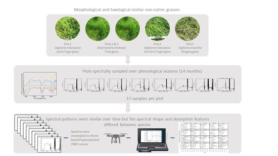
:The miniaturisation of hyperspectral sensors for use on drones has provided an opportunity to obtain hyper temporal data that may be used to identify and monitor non-native grass species. However, a good understanding of variation in spectra for species over time is required to target such data collections. Five taxological and morphologically similar non-native grass species were hyper spectrally characterised from multitemporal spectra (17 samples over 14 months) over phenological seasons to determine their temporal spectral response. The grasses were sampled from maintained plots of homogenous non-native grass cover. A robust in situ standardised sampling method using a non-imaging field spectrometer measuring reflectance across the 350–2500 nm wavelength range was used to obtain reliable spectral replicates both within and between plots. The visible-near infrared (VNIR) to shortwave infrared (SWIR) and continuum removed spectra were utilised. The spectra were then resampled to the VNIR only range to simulate the spectral response from more affordable VNIR only hyperspectral scanners suitable to be mounted on drones. We found that species were separable compared to similar but different species. The spectral patterns were similar over time, but the spectral shape and absorption features differed between species, indicating these subtle characteristics could be used to distinguish between species. It was the late dry season and the end of the wet season that provided maximum separability of the non-native grass species sampled. Overall the VNIR-SWIR results highlighted more dissimilarity for unlike species when compared to the VNIR results alone. The SWIR is useful for discriminating species, particularly around water absorption.
1. Introduction
Grasslands are among the largest ecosystems in the world [1] and cover around 26% of the world’s total land area and 69% of the agricultural area [2]. Grasslands are recognised globally for their high biodiversity and social and cultural values, as well as their capacity to deliver multiple ecosystem services as parts of agricultural production [3]. Examples of valuable agricultural production from grasses include feed for cattle for meat or milk production as well as cereals for human consumption. However, the impact of introduced grasses on the natural environment can be dramatic. Non-native species can out-compete native species and reduce biodiversity [4], increase fuel loads altering fire regimes, and reduce woody cover [5,6,7,8]. In the twentieth century, many grasses were deliberately introduced into the tropical savannas of northern Australia with the intent of improving pastoral output [9]. However, these non-native grasses have the potential to become weeds [10], and the introduction of pasture species for trial in northern Australia has increased the weed flora for both agriculture and conservation sectors [11].
Reliable methods for detecting the spread of introduced grasses into native and rehabilitated landscapes could improve the management of affected areas [12]. The spectra of grasslands have been studied utilising ground or lab-based spectrometers (e.g., [13,14,15,16]), satellite remote sensing (e.g., [17,18,19]), and airborne data (e.g., [20,21,22]). Grass spectra have been studied in diverse climates and environments from alpine [15,23], to African rangelands [16], and seagrasses [24]. Some early spectral work on grasses in the visible-near infrared (VNIR) region (e.g., [13,14]) showed a relationship existed between spectral reflectance and biomass.
Several physical and chemical characteristics useful for grass discrimination have been studied using spectral data. Lignin concentration was found to be a useful index for nitrogen cycling rates [25] and could be detected at wavelengths 1256, 1555, and 1311 nm. However, other constituents, such as water, prevented successful characterisation [26]. A strong correlation between the spectral red-edge and grass leaf chlorophyll content was found [21]. The spectral properties important for crop/weed discrimination in the laboratory was reviewed and summarised as chlorophyll a: 435, 670–680, 740 nm; chlorophyll b: 480, 650 nm; α-carotenoid: 420, 440, 470 nm; β-carotenoid: 425, 450, 480 nm; anthocyanin: 400–550 nm; lutein: 425, 445, 475 nm; violaxanthin: 425, 450, 475 nm; water: 970, 1450, 1944 nm [27]. Lignin and cellulose concentrations in grasses have been found to be less variable than in woody plants, with grass lignin values significantly lower than woody plants and cellulose being higher [28].
Many laboratory studies explored biochemical relationships with grass spectra, like those for nitrogen (N). The spectral response of Cenchus ciliaris grass grown in a greenhouse under three levels of N supply over a four-week period was measured and found that an increase in N supply yielded a shift in the red edge position to longer wavelengths [29]. A three-band spectral algorithm to characterise the N concentration and biomass of winter wheat and found that the bands of spectral indices should be optimised based on specific spectral index formulation and specific experimental conditions as the bands suitable for spectral indices can change with experimental conditions [30]. Many other indices using plant spectra have been trialled to assess plant physiological processes in agriculture and ecological monitoring, and a recent summary using photochemical reflectance indices on pea plants can be found in [31].
Studies utilising non-imaging spectrometers have provided insight into the feasibility of spectral separation of vegetation. A GER1500 spectrometer (350–1050 nm) was used to determine distinct features of alpine wetland grasses between 717.80–1050 nm caused by Leaf-Area-Index (LAI) and chlorophyll content [15]. Species level identification was not possible, with 70 alpine wetland grass species pairs among 138 clearly classified within that spectral range [15]. Given the similar composition, and therefore spectral signature, of many grassland species, data at multiple wavelengths allows more robust characterisation of grassland species and their biophysical parameters [17]. Not surprisingly, the results of [32] found grass areas with low inter-species overlap were better suited to spectral detection than areas with frequent inter-species overlap. Some of this historical spectral work has been seasonal, for example [33], although most studies utilised only a few days of measurement at most [15,34,35].
Analysis of spectral information obtained from hyperspectral imagery is one potential non-destructive method for the detection and mapping of non-native grasses [36]. The recent miniaturisation of hyperspectral sensors and their use on drones [37,38] provides an opportunity for the collection of hyperspectral image data at spatial and temporal frequencies that can be used for identifying, mapping and describing characteristics of plant species, including non-native grasses, at an appropriate scale. Recently, drone-based sensors have been used to map grasses. Cereal grass variety mapping has been undertaken using a red-green-blue (RGB) sensor at a resolution of 12 mega-pixels (MP) [39]. Above ground biomass of pastoral grasses has been characterised with a RGB camera at a resolution of 20 MP and a multispectral camera combined with ground-based light detection and ranging (LiDAR) to measure grass height [40]. Hyperspectral snapshot cameras have been combined with “Structure from Motion” (SfM) computer vision techniques in agricultural crops for the estimation of biomass of barley (e.g., [41]).
The Supervising Scientist Branch within Australia’s Department of Agriculture, Water and the Environment (http://www.environment.gov.au/science/supervising-scientist (accessed on 11 February 2021)) is undertaking characterisation of the surrounding savanna ecosystem at Ranger uranium mine, located within northern Australia’s World Heritage-listed Kakadu National Park. Future monitoring will compare the vegetation, including the savanna reference ecosystem to the revegetated areas of the mine site as it progresses toward closure. The use of drones fitted with hyperspectral sensors will enable the collection of at-scale data in the reference ecosystem surrounding the mine site.
This research focused on understanding the spectral characteristics of grass species over time to inform the spatial and temporal resolution for data capture to maximise the likelihood of separating grass species by spectral response. In this paper, we assess the ability to spectrally discriminate between five taxological and morphologically similar non-native grass species from multitemporal spectra collected using a robust sampling method. Because VNIR scanners mounted on drones are currently more affordable than those also covering the shortwave infrared (SWIR), we resampled the in situ data to the VNIR range only to investigate whether or not the spectra could be differentiated without the SWIR response. These data were historical (2006–2007) but have not been published before, and no such data exists elsewhere. As we are developing and implementing a drone-based hyperspectral monitoring method for understorey grasses, an analysis of this in situ data and the lessons learnt from in situ sampling of homogenous plots became crucial and applicable to our knowledge for monitoring.
2. Materials and Method
2.1. The Study Area and Plot Design
Field measurements were undertaken across five plots, each of pure and dense grass cover at the Berrimah Farm agricultural research station near Darwin in the Northern Territory of Australia (Figure 1). Although the vegetation was not always photosynthetic, the percentage cover was always 100%. On each sample, any disturbance, pattern of distribution and homogeneity (percent) was recorded in the metadata.
The climate of the study site is monsoonal wet-dry tropical with mean annual temperatures ranging from 23.2 °C to 32.1 °C (extremes from 10.4–38.9 °C) [42]. Climate records extending from 1963 show an average yearly rainfall of 1752 mm, with most of the precipitation falling between December and March. There is a distinct dry season, with minimal rainfall from May to September (Figure 2), on average.
Three species of non-native grasses used in the agricultural industry were represented over five sites: Brachiaria humidicola (Tully grass), Digitaria milanjiana (varieties Jarra Finger grass and Arnhem Finger grass), and Digitaria eriantha (Pangola grass). There were two replicates of B. humidicola and D. milanjiana. The scientific names of these grasses have experienced many botanical name changes, and the current naming conventions used here were supported by the Principal Pastures Agronomist in Darwin [44]. The scientific, common names and a representative photo are supplied for each of the sites at Berrimah Farm (or BF) (Table 1). The five sites are labelled BF01–05. See Figure 3 for representative plot photos where the spectral sampling was undertaken.
While many grasses look alike, there are potential spectral differences that may assist in discrimination based on differences such as textural features, pigment content and habit. Here we studied the spectra of five morphologically similar grasses and subsequently, provide an overview of the structure and appearance of the grasses and any features that may enhance (or confuse) the spectral separability of these species. The cultivar varieties of D. milanjiana (Jarra finger and Arnhem finger grass of BF01 and BF04, respectively) are used interchangeably [45]. D. milanjiana (BF01 and BF04) and D. eriantha (BF05) are both variable and perennial species [46]. The only consistent difference is that the nerves of the lower lemma are smooth in D. eriantha, and scaberulous in D. milanjiana [46,47]. Although the Digitaria species (BF01, 04, and 05) in this study are morphologically and structurally similar [48,49,50,51], there are some subtle differences. Arnhem Finger Grass (BF04) has a distinct tussock habit and is green, whereas Jarra Finger Grass (BF01) has runners and can be dark green and purple coloured, and Arnhem Grass (BF04) has a leafier appearance when compared with D. eriantha (Pangola Grass or BF05) [51]. B. humidicola (BF02 and 03) is also a perennial and is strongly stoloniferous and rhizomatous and this cultivar, known as Tully grass, has longer leaf blades (up to 25 cm long) than most other members of the species [46].
2.2. Field Data Collection
Five plots, each of 100% homogenous grass, measuring 2 × 2 m were marked out with star pickets and tape. The plots were easily accessible and could be sampled in a couple of hours around noon on a cloud-free day. The plots were close together (between 10 and 300 m), with similar soils and other environmental factors, like rainfall distribution. The five plots were sampled regularly, although not always fortnightly, for twenty-one visits over 14 months. Data capture dates are provided in Table S1. The sample dates were from the late dry season to the early wet season, specifically September through to late November 2006. There was a break in sampling over the wet season due to monsoonal rains and cloudiness. Sampling resumed in the late wet season (April) and occurred approximately fortnightly until early next wet season of November 2007.
Spectral sampling was undertaken using a FieldSpec® Pro-FR Analytical Spectral Device (ASD Inc., now Malvern Panalytical), with a spectral range of 350–2500 nm (spectral resolution of 3 nm at 700 nm, 10 nm at 1400/2100 nm). The detailed method for spectral sampling is provided elsewhere [52,53]. In summary, three replicates within a plot were taken from each plot on each sampling date. Target measurements were acquired with the operator positioned on the opposite side of the target to the sun in the solar principal plane. All measurements were made at a sensor zenith angle of 0° (nadir) with an optical 8° field-of-view (FOV). Spectral sampling was consistently undertaken from a pole height of 2 m height above the ground, which provided an approximate 28 cm diameter ground-field-of-view (GFOV). The spectra were normalised against a white reference (WR), in this case a 25 × 25 cm Spectralon (>99% reflectance) panel. The WR panel was situated 1 m from ground level. In situ WR measurements were made positioned on the side of the target point opposite the sun from a height of 2 m above ground level providing an approximate 14 cm diameter FOV (given the 1 m difference between FOV and panel) as shown in Figure 4. Meteorological data, measurement metadata, cover descriptions and photographs of the sky were recorded with each spectral measurement. Where environmental conditions changed during sampling, for example, an increase in wind velocity, sampling ceased. Sites not sampled on that day were sampled at the next opportunity, usually the next day.
A solar radiance spectrum followed by a WR spectrum (25 averages) was measured and saved. Immediately after the WR reading, three spectral averages (a, b, and c) were taken at each plot on each sample day [52,53]. To measure the three spectral averages, the stabilising pole was rotated horizontally 90° from the WR panel, and two additional sets of spectra were obtained by rotating the stabilising pole 60° and 30° sequentially. After the three target spectral samples were measured, the stabilising pole was positioned over the WR panel, and another WR reflectance measurement was taken to monitor for unrealised solar changes during target sampling. If there was variation in the WR readings between the spectral sampling, the measurements were repeated or abandoned if conditions were not ideal. Metadata on atmospheric conditions (clouds, smoke, haze, humidity, wind, and temperature), the hemispheric contribution (target texture and surrounds), standardised photographic recording of the sky and information on the target were also recorded.
Basic meteorological data, including rainfall, daily global exposure and daily maximum temperatures were obtained for Berrimah from the Bureau of Meteorology [43], covering the spectral sampling periods. While it was expected that most of the rainfall occurred in the wet season, we wanted to determine whether any showers occurred in the dry season that may align with any unexpected greening of grasses.
2.3. Data Analysis
Spectra were imported into a Spectral Analysis and Management System (SAMS) [54] database and sorted into folders by date. The standard deviation of the three spectral averages from each plot for each date were calculated, and the averages plotted. Spectral averages were exported into a spectral library in ENVI software (Harris Geospatial Solutions, Broomfield, Colorado). Endmember data were resampled to eliminate atmospheric water noise between 1346–1420 nm, 1800–1961 nm and longer than 2384 nm due to a loss of signal to noise ratio resulting from fibre optic cable length (5 m). The spectra were represented and graphed as reflectance values (0–0.65). A continuum removal (CR) [55] was applied to the spectra. CR is used to normalise reflectance spectra so individual absorption features can be compared from a common baseline. The continuum is removed to isolate individual absorption processes by dividing it into the reflectance spectrum. While CR is typically used as a diagnostic tool in narrow absorption features of mineral spectra, application to broader regions of the spectrum with vegetation have been demonstrated (56). We wanted to compare the common absorption features of vegetation in the VNIR, including chlorophyll as well as features in the SWIR, such as water. To eliminate false absorption detection due to noise, all CR absorptions below the threshold of 0.001 were excluded from the results.
Spectral Feature Fitting (SFF) [56] is an absorption feature-based method that matches spectra using a least squares technique after the continuum is removed from the spectra. While the SFF algorithm is often used in the minerals industry, because it is sensitive to subtle absorption features, it is useful here where the shape and magnitude of the spectra are similar. The SFF provided a Feature Fitting distance for each plot against the other plots sampled on the same date where a score closer to 1.0 indicated a closer match than those of lower scores. The range was 0–1. The Feature Fitting results were graphed in pairs. Each input spectrum was graphed against the other four plots of data by sampling period. Reflectance data were then resampled to the 400–1000 nm range (125 bands) to match the spectral range including band numbers and width of a currently available commercial VNIR hyperspectral scanner suitable for mounting on drones. CR and the SFF method were reapplied to the VNIR data only. This data analysis could be used to determine whether the SWIR region is desirable or essential for grass separation in the future.
3. Results
3.1. Meteorological Data
Figure 5a shows daily rainfall (mm) and the spectral sampling dates. Most of the rainfall occurred in the wet season when spectral sampling was not undertaken. Some rainfall can be observed during the sampling period. Daily maximum temperature (°C) (Figure 5b) was not as variable as rainfall, but slight decreases in temperature associated with dips in daily global solar exposure (cloudiness) with a slight decrease in temperature were observed (Figure 5b). There were some overcast days around the dates of spectral sampling, but no fieldwork occurred on cloudy days.
3.2. Summary Statistics
Summary statistics (Figure 6) of the total dataset show that the maximum magnitude of reflectance of the grasses was approximately 55%. The absorption features were most obvious in the CR spectra. The maximum values showed a characteristic dry spectrum in the visible region (lack of chlorophyll absorption) and a sharp increase in reflectance at the red edge, attributed to healthy green vegetation. The minimum reflectance curve (Figure 6a) highlights strong absorption features in the visible region due to chlorophyll (which increases in reflectance magnitude with decreasing chlorophyll) and a rather featureless increase in reflectance in the near-infrared, typical of drying vegetation. All spectra show absorptions centred around 1444 and 1965 nm as a result of cellular water. Referring to the CR spectrum in Figure 6b, by average, the electron transitions due to chlorophyll are centred at 492 and 675 nm. The centre of absorption ranged from 501 and 703 nm, respectively (Figure 6b). The red edge starting point was at 678 nm, with the slope crossing over between the minimum and mean average statistics. The green region peaked at 548 nm. Other generalised absorptions were centred at 972 nm (OH bend likely due to water and starch in the spongy mesophyll), around 1196 nm (variable) (OH bend likely due to lignin), 1725 nm (CH stretch likely due to cellulose, sugar and starch), 2094 nm (variable) (OH stretch likely due to sugar and starch) and 2270 nm (C-H stretch, O-H stretch, CH2 bend CH2 stretch due to cellulose sugar and starch) [57].
3.3. Temporal Analysis of the VNIR-SWIR Data–Reflectance and CR over Phenology
The temporal spectral response of the five grasses over select dates are shown in Figure 7. The full dataset of seventeen samples over time is displayed in Table S2. There was spectral pattern replication over the full dataset, so the selected results presented here describe the different spectral responses with phenological change. Spectra in Figure 7 are displayed as (a) reflectance, and, (b) CR stacked for clarity. The absorption positions from the CR are described here and graphed in Table S3.
Generally, the spectral patterns of the grass plots were similar over time, and this was not unexpected due to the common spectrally active compounds comprising these closely related grass species. Differences were attributed to well-known spectral features including the magnitude and position of chlorophyll absorption features, the red edge, the increase in slope in the near-infrared for senescing vegetation and the absorption features throughout the infrared, predominantly attributed to water content. The reflectance spectra displayed a characteristic green vegetation curve in the wet season with strong chlorophyll absorption in the blue and red regions intercepted by a small peak in the green, a strong red edge, maximum reflectance in the near-infrared and water absorptions in the infrared. As grass states moved toward senescence in the dry season, there were shifts in spectra resulting from reduced chlorophyll absorption, including a much-decreased red edge (magnitude) and less reflectance magnitude overall. Towards the very end of the dry season, the vegetation completely dried out and showed a spectrally featureless signature in the VNIR that increased in reflectance magnitude into the near-infrared. Absorption features became apparent in the SWIR, likely due to cellulose, sugar, lignin or starch.
3.3.1. Spectra of the Late Dry Season. Sample Dates (1–5) –26/09 (1), 9/10 (2), 30/10 (3), 15/11 (4), 30/11 (5)
The spectra from the first three sample dates in the late dry season (26 September, 9 October, and 30 October) displayed similar spectral reflectance profiles and absorption features for all grass species over this time (S2). The spectra for 9 October (sample date 2) (Figure 7) represent the general spectral shape over this time period. The grasses were senescent at the end of the dry season, and there was a general lack of pigmentation absorptions; however, some water absorption features remained, centred at 1443 and 1965 nm. These absorptions were at the same position for all grasses with the greatest depth for B. humidicola (BF02 and 03), with less absorption depth for D. milanjiana (BF01 and 04). D. erintha (BF05) displayed a decreased reflectance magnitude in the VNIR (Figure 7 and Table S2) when compared to the other four plots of grasses. The absorption position graph in S3 highlights a small absorption (<0.01%) at 1156 nm for one plot of B. humidicola (BF02), that is probably representative of leaf equivalent water thickness for all grasses. This feature was not picked up in the absorption feature processing for the other plots of grasses at the threshold used but can be observed in the spectral plots. All spectra showed a small absorption feature centred at 1725 nm, probably due to the presence of cellulose in the leaves [57].
The spectra from sample times 4 and 5 in mid-late November (Table S2) were similar, so sample date 4 (15 November) was used as a representative from this timeframe (Figure 7). The spectra of the grasses were measured after two rainfall events of less than 20 mm each (see Figure 5). There was a slight greening of grasses after this rainfall that is evident in the spectra. The spectra from the two plots of D. milanjiana (BF01 and BF04) were similar. They displayed chlorophyll absorptions centred at 502 and 678 nm and had intense water absorptions at 1446 nm that were broader in width compared to the spectra from the other three grass plots. By contrast, B. humidicola (BF02, 03) and D. eriantha (BF05) did not show strong chlorophyll absorption or red edge development, and the ~1450 nm water absorption was much broader. By late November, the B. humidicola (BF02, 03) and D. eriantha (BF05) had very weak chlorophyll absorptions (Tables S2 and S3). The spectra for plots D. milanjiana (BF01 and 04) displayed a small but apparent absorption at ~1153 nm. The similar absorptions seen in the D. milanjiana spectra have been highlighted in the position feature plot (Table S3).
3.3.2. Spectra of the Late Wet Season/Early Dry Season. Sample Dates 11/4 (6), 23/4 (7), 10/5 (8), 22/5 (9), 12/6 (10)
Spectral results of each species were similar over the late wet season in April and May (Table S2). Sample date 6 (11 April) was selected to represent this time frame (Figure 7) where overall the grasses displayed a typical green vegetation spectral response. Although all grasses displayed a typical green plant signature, differences were evident. The D. eriantha (BF05) spectrum showed a decreased reflectance magnitude compared to the spectra from the other plots, followed by a loss of chlorophyll and water absorption over time (Table S2). The D. milanjiana, cv. Arnhem finger grass (BF04) spectra consistently displayed the highest reflectance magnitude over this sampling period. The two plots of B. humidicola (BF02 and BF03) were most similar across the full wavelength range, and this species had the lowest reflectance magnitude in the SWIR and lesser water absorption intensities compared to the other species. The spectra of BF01 dropped in the VNIR reflectance magnitude compared to the same grass species in BF04 (Figure 7). The absorption position plot (Table S3) showed all spectra had the same absorptions; however, with different intensities that were evident also in the spectra (Figure 7).
By 12 June (sample date 10), the spectra for mixed species (D. milanjiana, B. humidicola and, D. eriantha or BF01, BF02, and BF05) lost the chlorophyll absorption features (around 493 and 674 nm) and displayed reduced water absorption intensity (Figure 7 and Table S3). Only BF03 and BF04 displayed the characteristics of a typical green vegetation spectra, despite these being different grass species. These results were explained by notes in the metadata, which described BF01 and BF02 as dead and dry and that uncontrolled cattle had knocked over the fence and trampled the grass which resulted in less than 100% homogenous vegetation cover with patches of bare ground making these spectra invalid and leaving only BF03–05 to analyse for the remaining dry season.
3.3.3. Spectra of the Dry Season. Sample Dates 18/7 (11), 1/8 (12), 6/9 (13), 21/9 (14), 4/10 (15), 5/10 (16) 26/11 (17)
It is difficult to make conclusions about the spectra of BF01 and BF02 during July-September because of the impact from cattle. Referring to BF03–05 only (Figure 7 and Table S2), the lowest reflectance magnitude in the VNIR is representative of BF05 during July–August. The absorptions in the leaf structure region of the spectrum (750–1300nm) are greater for BF03 compared to BF04. By mid-late September, all species show a drying signature.
Rainfall totalling 28.2 mm fell in late September and by early October (sample date 15), some green flush had occurred for the D. milanjiana plots, likely in response to the water. B. humidicola (BF02) also displayed a slight green up response in the spectra despite being previously disturbed. The spectra of the same species, B. humidicola, showed less chlorophyll absorption than D. milanjiana. Absorptions centred at 973 nm and 1163 nm were strongest in B. humidicola, but present and less intense in D. milanjiana. These absorptions were probably attributed to O-H bend due to water, cellulose or starch [57]. Plots BF01 and BF02 were sampled on the 15 October and BF03 on the 17 October (refer to Table S1). There were heavy showers before the 17 October, so the spectral response of BF03 was likely in response to the rainfall event.
At the end of November (see Table S2), the spectral results were overlapping between different genera. The metadata details that BF02 was “flushing and green and healthy from recent rains” whereas BF03 was described as “50% senesced and 50% green” despite these plots being of the same two species located in close proximity. The metadata described the grass of BF02 as mostly green grass, with a large bare compacted patch in the middle of the plot as a result of previous disturbance from cattle. The appearance of BF03 was very patchy with approximately 50% green flushed grass and 50% dried brown grass. This early wet season time, when showers are falling, but the monsoon rains have not yet set in, was found to not be a useful timing of year to distinguish these grass species.
3.4. Spectral Feature Fitting Results
The Spectral Feature Fitting results compared each plot to the other four plots by sampling date and was graphed for the full spectrum covering the VNIR and SWIR in Figure 8. The table of results can be found in Table S4. To align with hyperspectral VNIR sensors currently suitable for mounting on drones that tend to be more affordable than those that incorporating VNIR-SWIR sensors, the spectra were resampled to the VNIR only and the SFF results are provided in Figure 9 and Table S5. A value of 1.0 represented the same spectrum and approaching towards 0.0 represented an increasingly less similar set of spectra.
Overall, the VNIR-SWIR results in Figure 8 highlighted more dissimilarity at times for more unlike species when compared to the VNIR result in Figure 9. In the VNIR-SWIR results, generally, the B. humidicola (BF02 and 03) were more similar than the Digitiaria plots. Further, the D. milanjiana varieties (BF01 and BF04) were more similar than the D. eriantha (BF05). An exception was after the dry season of 2007, when cattle disturbed plots BF01 and BF02. It was straight after the wet season rains, around April, that the lowest values were seen for more dissimilar vegetation grasses across the VNIR-SWIR region (Figure 8).
The VNIR-SWIR feature fitting separability (Figure 8) graphically showed the high similarity of the D. milanjiana plots (BF01 and 04) with high scores often around 0.9. These pairs scored the highest spectral similarities (from 0.959–0.983) (S3). During early October (9 October 2006) and late November (30 November 2006) BF01 and BF04 had the same and similar scores, respectively, to BF02 indicating similar spectra across the full range. The CR profile (Figure 7) highlights the similar absorptions of BF04 and BF02 in the near-infrared, whereas longer of 1000nm, BF01 and BF04 had similar reflectance magnitude, illustrating a shortcoming of the Feature Fitting method. The impact of cattle affects scores from 12 June 2007.
The B. humidicola plots (BF02 and BF03) scored high spectral similarities (0.910–0.989) (S3), although were not always the most similar over the VNIR-SWIR. For example, on 30 November 2006, and from 6 December 2007 to 1 August 2007 inclusive (due to cattle) and again in the late dry season of 2007 (15 October 2007 and 26 November 2007) and this is represented in Figure 8.
BF05 most often scored closer to BF01 and BF04 (of the same genus Digitaria), than to the B. humidicola of BF02 and BF03 and this is apparent in Figure 8 where all values are greater than 0.9 (for BF01–04, BF01–05, BF04–05, BF05–01 and BF05–04). A shortcoming of the Feature Fitting method is that unlike species not ranking the highest as pairs are at times still showing high similarities across the full spectrum.
With the VNIR only, there is much more mixing with species showing similar high scores with unlike species with the exception of late April 2007. The BF01–04 were consistently above 0.95, although at times there was a close match to BF05.
The VNIR only data (Figure 9) showed that plots of the same species D. milanjiana (BF01 and BF04) and B. humidicola (BF02 and BF03) were the most similar overall. BF01 and BF04 were similar in the late dry, and the early wet, and, BF02 and BF03 were similar in the early wet. Different species dropped in score nearing 0.8 at times, indicating more spectral separability. In early October 2006, D. eriantha (BF05) was most dissimilar to B. humidicola (BF02 and BF03) in the VNIR results (Figure 9). However, based on the Feature Fitting distance over the full spectrum (Figure 8), B. humidicola (BF02 and BF03) were not always the most similar spectra over these dates. When utilising just the VNIR, B. humidicola BF02 and BF03 were most similar; however, this excluded the water absorption and other features that were apparent in the SWIR data. In late November, after rainfall showers, D. milanjiana (BF01 and BF04) were similar (Figure 7, Figure 8 and Figure 9). After the main wet season rains in April, B. humidicola (BF02 and BF03) were most similar across the full wavelength range. By October 2007, the spectra of the same species: B. humidicola (BF02 and BF03,) showed less chlorophyll absorption and their statistics were more similar in both the VNIR-SWIR and VNIR only, suggesting this grass is variable from the other species even in the early wet season.
4. Discussion
The spectral patterns of the grass plots were generally similar over time, and this was not unexpected due to the common compounds making up all plants and particularly that of closely related grass species. However, there were differences in spectral shape and absorption features. A summary is provided below in Table 2. In the late dry season (October), the spectral patterns were similar, and it was the water absorption depths and overall reflectance magnitude that were the distinguishing features. The obvious distinguishing feature during this drying stage was the higher reflectance magnitude in the SWIR for D. milanjiana compared to the other vegetation species. It was unexpected that this phenological period could be used to differentiate species based on spectral response. In the very late dry season (mid-November), rainfall showers prior to the onset of wet season rains resulted in a species greening up before other grasses, and this was a distinguishing response. In this example, the plots of D. milanjiana displayed a similar spectral response but separable from the other species measured due to chlorophyll and water absorptions. By contrast, B. humidicola and D. eriantha did not show chlorophyll absorption or the development of a red edge during this stage of rainfall showers. D. eriantha was distinctly different from the other species and displayed the lowest reflectance magnitude measured during the late wet season (e.g., early April). At this time frame, all species had similar absorptions positions with different intensities. D. milanjiana (cv Arnhem Finger grass–BF04) displayed the highest reflectance magnitude. Biologically, only very subtle differences based on the texture of the lower lemma distinguish this species from the other plots. Here we found subtle spectral differences of the Digitaria genus grasses in this study, despite high within-species variability being documented [48,49,50,51].
Results from D. milanjiana and B. humidicola showed that grasses of the same species had the highest similarity over many of the sampling dates. Exceptions to this were a result of disturbance due to feral animals. Another exception was between the B. humidicola plots during May, where all grasses were green; however, BF02 showed a lower reflectance magnitude in the visible region, a red edge at longer wavelengths, and a very strong absorption at 978 nm. While both plots of the same species were 100% homogenous and very green, one of these plots (BF02) was in the last stages of seeding, whereas the other plot had finished seeding. It is not known whether this was due to an agricultural trial such as fertiliser application or natural variability.
At the end of the wet season, around April, the grasses showed the greatest separability, and it was the VNIR-SWIR (Figure 8), rather than the VNIR (only) (Figure 9) that showed the best separation based on absorption features. Currently, VNIR hyperspectral sensors are the most cost-effective for use on drones. For example, the Headwall VNIR system [58], Ocean Optics STS [59] and Corning MicroHSI SHARK [60] have been utilised in agricultural settings. While miniaturised SWIR sensors are available (e.g., [61]), they are more cost-prohibitive but may become more readily accessible as technology advances, and SWIR systems become more affordable. Given the similar composition, and therefore spectral signature, of many grassland sites, data at multiple wavelengths allow more robust characterisation of grassland species and their biophysical parameters [17]. The SWIR region is useful particularly for indicating cellular water but also smaller absorptions that may be due to sugar or cellulose, as well as the rise in reflectance magnitude as species senesce.
Here we compared five homogenous plots of grasses. Many grass species in an alpine setting were measured, but species identification was difficult [15]. It is acknowledged that here, we might find more confounding results if further grassland species were introduced into the spectral matrix. Further, we sampled from homogenous plots. Grasses with low interspecies overlap were better suited to spectral detection than areas with frequent inter-species overlap [32], and we acknowledge that the spectral setting of these grasses in a mixed pasture may be more challenging, if not impossible.
Continuum removal is a numerical method used to investigate the physical basis and spectral features of plants, often relating to foliar chemistry. Numerous works demonstrate the advantage of utilising the full spectrum with CR over spectral indices (e.g., [29,62]). CR has the advantage of utilising the whole spectrum, rather than simplifying the data (e.g., [63,64]). In this case, we have focused on the spectral differences based on results over the full spectrum. It can be expected when extrapolating spectral results from drone-based measurements that appropriate bands used in spectral indices may need to change with experimental conditions and environmental factors (such as substrate type or moisture availability) [29,64]. When using spectral index formulation under specific experimental conditions, determining suitable bands was challenging with changing experimental conditions [30]. The CR is used in Spectral Feature Fitting (SFF). SFF compares the absorption features of spectra to a known reference spectrum. It is an absorption-features method and a common strategy for hyperspectral analysis to discriminate ground targets [65]). While the SFF algorithm is often used in the minerals industry, because it is sensitive to subtle absorption features, it is useful here where the shape and magnitude of the spectra are similar. Spectral Features are commonly analysed in vegetation spectra (e.g., [15,65,66,67]).
Several introduced grasses have already become declared weeds in the Northern Territory, for example, Andropogon gayanus (or gamba grass) [8,68,69]. With the spread of such weeds, it is important that the spectral response of these non-native species, combined with the textural response from drone- based platforms is further researched so that any detection of these grasses can be managed appropriately.
In this dataset, the very late dry season could be used for the spectral separability of the D. milanjiana species because its chlorophyll absorption and deep water absorption, as well as the higher reflectance magnitude in the SWIR which was present because this species greened up post rainfall showers before the other species showed any spectral response to rainfall. Using this phenological response would require knowledge about local rainfall, and the existence of a localised automatic weather station to detect rainfall and inform deployment of appropriate sensors on drones.
The disturbance of vegetation by cattle, and perhaps by other introduced species, hinders the ability to discriminate between species spectrally.
5. Conclusions
The data capture design, in this case, reduced systematic uncertainties. The grasses were all grown in the same substrate and received the same rainfall. The plots were regularly inspected to ensure homogeneity of cover. The ability to measure three replicates, each with 25 averaged samples meant there was certainty that the plot average was representative of the species. All measurements could be made within an hour of sampling (around noon), so that irradiance measures were similar. If an extraneous event occurred, for example, that winds picked up or clouds emerged, the measurement could be abandoned and repeated at the next opportunity.
The spectral measurement of five plots of taxological and morphologically identical and/or similar species over phenological stages was undertaken. The phenological stage that maximum separability is detected will depend on the species. Maximum separability may not be growth or seasonal stage, but rather a response to flushing after rainfall showers or due to disturbance from animals, such as cattle. Unexpectantly, in the tropical savanna environment, maximum separability may be in the very late dry season with the onset of rainfall showers where similarities between species and differences from genera were measured. Standardised procedures to obtain reference spectra are particularly valid when measurements are made from ground-based spectrometers, and it is expected that these factors will need to be considered when spectrally sampling from drone-based platforms.
Even more applicable to drone-based acquired spectral data compared to ground-based spectral data over homogenous plots will be the consideration of factors affecting spectral measurements. These include data collection design (timing of data collection, method of data collection including geometry, and the scale and number of overpasses considering spatial and temporal variability), calibration (of references and spectrometer), instrument settings (dark current and white reference integration), illumination and viewing geometry (sun angle, wind speed and direction, cloud cover and type, temperatures and humidity, aerosols/smoke/haze), and the properties of the target (species, homogeneity, localised conditions, layering, cover, phenology, health, form, and texture).
Characterising grasses from hyperspectral data mounted on drones may be beneficial over ground-based sampling because nadir 3-band imagery can be displayed, and texture relating to species-specific morphology as well as phenological stages such as flowering may be identified and used to aid separability. Further, hyperspectral data can be used in conjunction with other sensor types, such as LiDAR, that are suited to measure structural characteristics.
Supplementary Materials
The following are available online at https://www.mdpi.com/2072-4292/13/4/738/s1, Table S1: Spectral sampling dates at Berrimah Farm. Table S2: Seventeen spectral samples over time of the five grass species. a) Reflectance, b) offset for clarity and c) continuum removed (CR) offset for clarity. Table S3: Absorption (Band Depth of absorption). The centre points based on the CR were 430, 490, 580, 620, 660, 930, 970, 1120, 1450, 1780, 1970, 2090 and 2270 nm). Table S4: Spectral Feature Fitting separability results (VNIR-SWIR). Table S5: Spectral Feature Fitting separability results (350–1000 nm).
Author Contributions
Conceptualization, K.P., T.W., R.B; methodology, K.P.; software K.P., D.L., A.E.; formal analysis, K.P. and D.L.; investigation, K.P.; resources, K.P. and R.B.; data curation, D.L.; writing—original draft preparation, K.P.; writing—review and editing, K.P., T.W. and R.B.; visualization, K.P., D.L. and E.S.; project administration, K.P., R.B., T.W. All authors have read and agreed to the published version of the manuscript.
Funding
This research received no external funding.
Institutional Review Board Statement
Not applicable.
Informed Consent Statement
Not applicable.
Data Availability Statement
Data is contained within the article or supplementary material (SM).
Acknowledgments
Geoff Carr undertook most of the spectral sampling. Berrimah Research Farm allowed access for in situ sampling of grasses.
Conflicts of Interest
The authors declare no conflict of interest.
References
- Oenema, O.; de Klein, C.; Alfaro, M. Intensification of grassland and forage use: Driving forces and constraints. Crop Pasture Sci. 2014, 65, 524–537. [Google Scholar] [CrossRef]
- O’Mara, F. The role of grasslands in food security and climate change. Annal. Bot. 2012, 110, 1263–1270. [Google Scholar] [CrossRef] [PubMed] [Green Version]
- Bengtsson, J.; Bullock, J.M.; Egoh, B.; Everson, C.; Everson, T.; O’Connor, T.; O’Farrell, P.J.; Smith, H.G.; Lindborg, R. Grasslands—More important for ecosystem services than you might think. Ecosphere 2019, 10, 1–20. [Google Scholar] [CrossRef]
- Ferdinands, K.; Beggs, K.; Whitehead, P. Biodiversity and invasive grass species: Multiple-use or monoculture? Wildlife Res. 2005, 32, 447–457. [Google Scholar] [CrossRef]
- Mack, M.C.; D’Antonio, C.M. Impacts of biological invasions on disturbance regimes. Trend. Ecol. Evol. 1998, 13, 195–198. [Google Scholar] [CrossRef]
- Brooks, M.L.; D’antonio, C.M.; Richardson, D.M.; Grace, J.B.; Keeley, J.E.; DiTomaso, J.M.; Hobbs, R.J.; Pellant, M.; Pyke, D. Effects of invasive alien plants on fire regimes. BioScience 2004, 54, 677–688. [Google Scholar] [CrossRef] [Green Version]
- Douglas, M.M.; Setterfield, S.A.; Rossiter, N.A.; Barratt, J.; Hutley, L. Effects of mission grass (Pennisetum polystachion (L) Schult.) invasion on fuel loads and nitrogen availability in a northern Australia tropical savanna. In Proceedings of the 14th Australian Weeds Conference; Wagga Wagga, New South Wales, Australia, 6–9 September 2004, Sindel, B., Johnson, S., Eds.; Charles Sturt University: New South Wales, Australia, 2004; pp. 179–181. [Google Scholar]
- Setterfield, S.A.; Rossiter-Rachor, N.A.; Hutley, L.B.; Douglas, M.M.; Williams, R.J. Biodiversity research: Turning up the heat: The impacts of Andropogon gayanus (gamba grass) invasion on fire behaviour in northern Australian savannas. Divers. Distrib. 2010, 16, 854–861. [Google Scholar] [CrossRef]
- Cook, G.; Dias, L. It was no accident: Deliberate plant introductions by Australian government agencies during the 20th century. Turner Review No. 12. Aust. J. Bot. 2006, 54, 601–625. [Google Scholar] [CrossRef]
- Grace, B.S.; Gardener, M.R.; Cameron, A.G. Pest or pasture? Introduced pasture grasses in the Northern Territory. In Proceedings of the 14th Australian Weeds Conference, Wagga Wagga, New South Wales, Australia, 6–9 September 2004; pp. 157–160. [Google Scholar]
- Lonsdale, W.M.; Lane, A.M. Tourist vehicles as vectors of weed seeds in Kakadu National Park, Northern Australia. Biolo. Conserv. 1994, 69, 277–283. [Google Scholar] [CrossRef]
- López-Granados, F. Weed detection for site-specific weed management: Mapping and real time approaches. Weed Res. 2010, 51, 1–11. [Google Scholar]
- Tucker, C.J. Asymptotic nature of grass canopy spectral reflectance. Appl. Optics. 1977, 16, 1151–1156. [Google Scholar] [CrossRef] [PubMed]
- Tucker, C.J. Spectral estimation of grass canopy variables. Remote Sens. Environ. 1977, 6, 11–26. [Google Scholar] [CrossRef]
- Bao, S.; Cao, C.; Chen, W.; Tian, H. Spectral features and separability of alpine wetland grass species. Spectrosc. Lett. 2017, 50, 245–256. [Google Scholar] [CrossRef]
- Schmidt, K.; Skidmore, A. Exploring spectral discrimination of grass species in African rangelands. Int. J. Remote Sens. 2001, 22, 3421–3434. [Google Scholar] [CrossRef]
- Ali, I.; Cawkwell, F.; Dwyer, E.; Barrett, B.; Green, S. Satellite remote sensing of grasslands: From observation to management. J. Plant Ecol. 2016, 9, 649–671. [Google Scholar] [CrossRef] [Green Version]
- Gómez-Casero, M.T.; Castillejo-González, I.L.; García-Ferrer, A.; Peña-Barragán, J.M.; Jurado-Expósito, M.; García-Torres, L.; López-Granados, F. Spectral discrimination of wild oat and canary grass in wheat fields for less herbicide application. Agron. Sustain. Dev. 2010, 30, 689–699. [Google Scholar] [CrossRef]
- Shoko, C.; Mutanga, O. Seasonal discrimination of C3 and C4 grasses functional types: An evaluation of the prospects of varying spectral configurations of new generation sensors. Int. J. Appl. Earth Obs. Geoinf. 2017, 62, 47–55. [Google Scholar] [CrossRef]
- Cho, M.A.; Skidmore, A.; Corsi, F.; Van Wieren, S.E.; Sobhan, I. Estimation of green grass/herb biomass from airborne hyperspectral imagery using spectral indices and partial least squares regression. Int. J. Appl. Earth Obs. Geoinf. 2007, 9, 414–424. [Google Scholar] [CrossRef]
- Pinar, A.; Curran, P. Technical note grass chlorophyll and the reflectance red edge. Int. J. Remote Sens. 1996, 17, 351–357. [Google Scholar] [CrossRef]
- Wang, Z.; Townsend, P.A.; Schweiger, A.K.; Couture, J.J.; Singh, A.; Hobbie, S.E.; Cavender-Bares, J. Mapping foliar functional traits and their uncertainties across three years in a grassland experiment. Remote Sens. Environ. 2019, 221, 405–416. [Google Scholar] [CrossRef]
- Yu, H.; Kong, B.; Wang, G.; Sun, H.; Wang, L. Hyperspectral database prediction of ecological characteristics for grass species of alpine grasslands. Rangel. J. 2018, 40, 19–29. [Google Scholar] [CrossRef]
- Fyfe, S.K. Spatial and Temporal Variation in Spectral Reflectance: Are Seagrass Species Spectrally Distinct? Limnol. Oceanogr. 2003, 48, 464–479. [Google Scholar] [CrossRef]
- Wessman, C.A.; Aber, J.D.; Peterson, D.L. An evaluation of imaging spectrometry for estimating forest canopy chemistry. Int. J. Remote Sens. 1989, 10, 1293–1316. [Google Scholar] [CrossRef]
- Wessman, C.A.; Aber, J.D.; Peterson, D.L.; Melillo, J.M. Remote sensing of canopy chemistry and nitrogen cycling in temperate forest ecosystems. Nature 1988, 335, 154. [Google Scholar] [CrossRef]
- Zwiggelaar, R. A review of spectral properties of plants and their potential use for crop/weed discrimination in row-crops. Crop Prot. 1998, 17, 189–206. [Google Scholar] [CrossRef]
- Asner, G.P. Biophysical and biochemical sources of variability in canopy reflectance. Remote Sens. Environ. 1998, 64, 234–253. [Google Scholar] [CrossRef]
- Mutanga, O.; Skidmore, A.K. Red edge shift and biochemical content in grass canopies. ISPRS J. Photogramm. Remote Sens. 2007, 62, 34–42. [Google Scholar] [CrossRef]
- Li, F.; Mistele, B.; Hu, Y.C.; Chen, X.P.; Schmidhalter, U. Optimising Three-Band Spectral Indices to Assess Aerial N Concentration, N Uptake and Aboveground Biomass of Winter Wheat Remotely in China and Germany. ISPRS J. Photogramm. Remote Sens. 2014, 92, 112–123. [Google Scholar] [CrossRef]
- Sukhova, E.; Sukhov, V. Relation of Photochemical Reflectance Indices Based on Different Wavelengths to the Parameters of Light Reactions in Photosystems I and II in Pea Plants. Remote Sens. 2020, 12, 1312. [Google Scholar] [CrossRef] [Green Version]
- Lopatin, J.; Fassnacht, F.E.; Kattenborn, T.; Schmidtlein, S. Mapping plant species in mixed grassland communities using close range imaging spectroscopy. Remote Sens. Environ. 2017, 201, 12–23. [Google Scholar] [CrossRef]
- Matson, P.; Johnson, L.; Billow, C.; Miller, J.; Pu, R. Seasonal patterns and remote spectral estimation of canopy chemistry across the Oregon transect. Ecol. Appl. 1994, 4, 280–298. [Google Scholar] [CrossRef]
- Cundill, S.L.; van der Werff, H.M.A.; van der Meijde, M. Adjusting Spectral Indices for Spectral Response Function Differences of Very High Spatial Resolution Sensors Simulated from Field Spectra. Sensors 2015, 15, 6221–6240. [Google Scholar] [CrossRef] [PubMed]
- Kattenborn, T.; Fassnacht, F.E.; Schmidtlein, S. Differentiating plant functional types using reflectance: Which traits make the difference? Remote Sens. Ecol. Conserv. 2019, 5, 5–19. [Google Scholar] [CrossRef] [Green Version]
- Marcinkowska-Ochtyra, A.; Jarocińska, A.; Bzdęga, K.; Tokarska-Guzik, B. Classification of Expansive Grassland Species in Different Growth Stages Based on Hyperspectral and LiDAR Data. Remote Sens. 2018, 10, 2019. [Google Scholar] [CrossRef] [Green Version]
- Hakala, T.; Markelin, L.; Honkavaara, E.; Scott, B.; Theocharous, T.; Nevalainen, O.; Näsi, R.; Suomalainen, J.; Viljanen, N.; Greenwell, C.; et al. Direct reflectance measurements from drones: Sensor absolute radiometric calibration and system tests for forest reflectance characterization. Sensors 2018, 18, 1417. [Google Scholar] [CrossRef] [PubMed] [Green Version]
- Saari, H.; Akujärvi, A.; Holmlund, C.; Ojanen, H.; Kaivosoja, J.; Nissinen, A.; Niemeläinen, O. Visible, very near IR and shortwave IR hyperspectral drone imaging system for agriculture and natural water applications. Int. Arch. Photogram. Remote Sens. Spat. Inf. Sci. 2017, XLII-3/W3, 165–170. [Google Scholar] [CrossRef] [Green Version]
- Constantinescu, C.A.; Herbei, M.V.; Sala, F. Characterisation of some varieties of cereal grasses on the basis of spectral information from aerial images. Res. J. Agric. Sci. 2017, 49, 85–94. [Google Scholar]
- Michez, A.; Lejeune, P.; Bauwens, S.; Herinaina, A.A.L.; Blaise, Y.; Castro Muñoz, E.; Lebeau, F.; Bindelle, J. Mapping and Monitoring of Biomass and Grazing in Pasture with an Unmanned Aerial System. Remote Sens. 2019, 11, 473. [Google Scholar] [CrossRef] [Green Version]
- Aasen, H. The Acquisition of Hyperspectral Digital Surface Models of Crops from UAV Snapshot Cameras. PhD thesis, Universität zu Köln, Köln, Germany, 2016. [Google Scholar]
- BOM Bureau of Meteorology, Climate Data Online. Available online: http://www.bom.gov.au/jsp/ncc/cdio/weatherData/av?p_nccObsCode=122&p_display_type=dailyDataFile&p_startYear=&p_c=&p_stn_num=014015 (accessed on 22 July 2020).
- Bureau of Meteorology (BOM) Mean Rainfall of Berrimah Farm. Available online: http://www.bom.gov.au/climate/data/ (accessed on 1 April 2020).
- Cameron, A.; Principal Pastures Agronomist, Darwin. Personal communication, 29 April 2019.
- Beggs, K.E. Effects of exotic pasture grasses on biodiversity in the Mary River Catchment, Northern Territory. PhD thesis, Charles Darwin University, Darwin, Australia, 2010. [Google Scholar]
- Tropical Forages. Available online: https://www.tropicalforages.info/text/entities/digitaria_eriantha.htm and https://www.tropicalforages.info/text/entities/digitaria_milanjiana.htm (accessed on 1 May 2019).
- Cook, B.G.; Pengelly, B.C.; Brown, S.D.; Donnelly, J.L.; Eagles, D.A.; Franco, M.A.; Hanson, J.; Mullen, B.F.; Partridge, I.J.; Peters, M.; et al. Tropical Forages: An Interactive Selection Tool CSIRO, DPI&F (Qld), CIAT and ILRI, Brisbane, Australia. Available online: https://www.tropicalforages.info/text/intro/index.html (accessed on 15 February 2021).
- Cameron, A.G. Pangola Grass (Digitaria eriantha) Agnote, No, E35, Department of Primary Industry, Fisheries and Mines Northern Territory Government. January 2013. Available online: https://industry.nt.gov.au/__data/assets/pdf_file/0015/233430/306.pdf (accessed on 15 February 2021).
- Cameron, A.G. Tully (Brachiaria humidicola). Agnote, No. E31, Department of Primary Industry, Fisheries and Mines. Northern Territory Government. January 2013. Available online: https://dpir.nt.gov.au/__data/assets/pdf_file/0005/233438/550.pdf (accessed on 15 February 2021).
- Cameron, A.G. Arnhem Finer Grass (Digitaria swynnertonii), Agnote, No. E63, Northern Territory Government. February 2019. Available online: https://industry.nt.gov.au/__data/assets/pdf_file/0005/233537/725.pdf (accessed on 15 February 2021).
- Cameron, A.G. Jarra Finer Grass (Digitaria milanjiana cv Jarra), Agnote, No. E55, Northern Territory Government. August 2010. Available online: https://industry.nt.gov.au/__data/assets/pdf_file/0019/233209/684.pdf (accessed on 15 February 2021).
- Pfitzner, K.; Bollhöfer, A.; Carr, G. A standard design for collecting vegetation reference spectra: Implementation and implications for data sharing. J. Spat. Sci. 2006, 52, 79–92. [Google Scholar] [CrossRef]
- Pfitzner, K.; Bartolo, R.; Carr, G.; Esparon, A.; Bollhöfer, A. Standards for Reflectance Spectral Measurement of Temporal Vegetation Plots; Supervising Scientist Report 195; Department of Sustainability, Environment, Water, Population and Communities: Darwin, NT, Australia, 2011. Available online: https://www.environment.gov.au/science/supervising-scientist/publications/ssr/standards-for-reflectance-spectral-measurement-of-temporal-vegetation-plots. (accessed on 15 February 2021).
- Rueda, C.A.; Wrona, A.F. SAMS Spectral Analysis and Management System Version 2.0 User’s Manual. Centre for Spatial Technologies and Remote Sensing, Department of Land, Air and Water Resources, University of California, Davis: Davis, CA, USA. 2003. Available online: https://storage.googleapis.com/google-code-archive-downloads/v2/code.google.com/cstars-sams/SAMS%202.0%20User%20Manual.pdf (accessed on 15 February 2021).
- Clark, R.N.; Roush, T.L. Reflectance spectroscopy: Quantitative analysis techniques for remote sensing applications. J. Geophys. Res: Solid Earth 1984, 89, 6329–6340. [Google Scholar] [CrossRef]
- Clark, R.N.; Swayze, G.A. Mapping minerals, amorphous materials, environmental materials, vegetation, water, ice and snow, and other materials: The USGS tricorder algorithm. In Summaries of the Third Annual JPL Airborne Geoscience Workshop (Volume 1, pp. 39–40); JPL Publication 92–14; Jet Propulsion Laboratory: Pasadena, CA, USA, 1995. Available online: https://popo.jpl.nasa.gov/pub/docs/workshops/95_docs/12.PDF (accessed on 15 February 2021).
- Curran, P.J. Remote sensing of foliar chemistry. Remote Sens. Environ. 1989, 30, 271–278. [Google Scholar] [CrossRef]
- Adão, T.; Peres, E.; Pádua, L.; Hruška, J.; Sousa, J.J.; Morais, R. UAS-based hyperspectral sensing methodology for continuous monitoring and early detection of vineyard anomalies. In Proceedings of the Small Unmanned Aerial Systems for Environmental Research, Vila Real, Portugal, 28–30 June 2017. [Google Scholar]
- Burkart, A.; Cogliati, S.; Schickling, A.; Rascher, U. A novel UAV-based ultra-light weight spectrometer for field spectroscopy. IEEE Sens. J. 2014, 14, 62–67. [Google Scholar] [CrossRef]
- Holasek, R.; Nakanishi, K.; Ziph-Schatzberg, L.; Santman, J.; Woodman, P.; Zacaroli, R.; Wiggins, R. The selectable hyperspectral airborne remote sensing kit (SHARK) as an enabler for precision agriculture. In Proceedings SPIE 10213, Hyperspectral Imaging Sensors: Innovative Applications and Sensor Standards Anaheim, Anaheim, CA, USA, 22 May 2017; p. 1021304. [Google Scholar] [CrossRef]
- Zhong, Y.; Wang, X.; Xu, Y.; Jia, T.; Cui, S.; Wei, L.; Ma, A.; Zhang, L. MINI-UAV borne hyperspectral remote sensing: A review. In Proceedings of 2017 IEEE International Geoscience and Remote Sensing Symposium (IGARSS), Fort Worth, TX, USA, 23–28 July 2017; pp. 5908–5911. [Google Scholar]
- Mitchell, J.J.; Glenn, N.F.; Sankey, T.T.; Derryberry, D.R.; Anderson, M.O.; Hruska, R.C. Spectroscopic detection of nitrogen concentrations in sagebrush. Remote Sens. Lett. 2012, 3, 285–294. [Google Scholar] [CrossRef]
- Curran, P.J.; Dungan, J.L.; Peterson, D.L. Estimating the foliar biochemical concentration of leaves with reflectance spectrometry: Testing the Kokaly and Clark methodologies. Remote Sens. Environ. 2001, 76, 349–359. [Google Scholar] [CrossRef]
- Shi, T.; Wang, J.; Liu, H.; Wu, G. Estimating leaf nitrogen concentration in heterogeneous crop plants from hyperspectral reflectance. Int. J. Remote Sens. 2015, 36, 4652–4667. [Google Scholar] [CrossRef]
- Pan, Z.; Huang, J.; Wang, F. Multi range spectral feature fitting for hyperspectral imagery in extracting oilseed rape planting area. Int. J. Appl. Earth Obs. Geoinf. 2013, 25, 21–29. [Google Scholar] [CrossRef]
- Kokaly, R.F.; Despain, D.G.; Clark, R.N.; Livo, K.E. Mapping vegetation in Yellowstone National Park using spectral feature analysis of AVIRIS data. Remote Sens. Environ. 2003, 84, 437–456. [Google Scholar] [CrossRef] [Green Version]
- Mutanga, O.; Skidmore, A.K.; Prins, H.H.T. Predicting in situ pasture quality in the Kruger National Park, South Africa, using continuum-removed absorption features. Remote Sens. Environ. 2004, 89, 393–408. [Google Scholar] [CrossRef]
- Rossiter-Rachor, N.A.; Setterfield, S.A.; Douglas, M.M.; Hutley, L.B.; Cook, G.D. Andropogon gayanus (gamba grass) invasion increases fire-mediated nitrogen losses in the tropical savannas of northern Australia. Ecosystems 2008, 11, 77–88. [Google Scholar] [CrossRef]
- Head, L.; Atchison, J. Governing invasive plants: Policy and practice in managing the Gamba grass (Andropogon gayanus)–bushfire nexus in northern Australia. Land Use Policy 2015, 47, 225–234. [Google Scholar] [CrossRef]
Figure 1.
Study site. Berrimah is a suburb of Darwin in the Northern Territory of Australia. There are five sites labelled Berrimah Farm (BF) or BF01-05. The five sites were within proximity of each other.
Figure 1.
Study site. Berrimah is a suburb of Darwin in the Northern Territory of Australia. There are five sites labelled Berrimah Farm (BF) or BF01-05. The five sites were within proximity of each other.

Figure 2.
Mean monthly rainfall (mm) at Berrimah Farm (1963–2019) (adapted from [43]).
Figure 2.
Mean monthly rainfall (mm) at Berrimah Farm (1963–2019) (adapted from [43]).

Figure 3.
The grass plots at Berrimah Farm (BF) (taken 23_01_2008). Plots BF01, BF04 and BF05 were of the same genus, Digitaria, with similar species/varieties and plots BF02 and BF03 were of the same species, Brachiaria humidicola.
Figure 3.
The grass plots at Berrimah Farm (BF) (taken 23_01_2008). Plots BF01, BF04 and BF05 were of the same genus, Digitaria, with similar species/varieties and plots BF02 and BF03 were of the same species, Brachiaria humidicola.

Figure 4.
Standardised setup. Photograph of Digitaria milanjiana (BF04) taken 11 April 2007 while the grass is still green after wet season rains.
Figure 4.
Standardised setup. Photograph of Digitaria milanjiana (BF04) taken 11 April 2007 while the grass is still green after wet season rains.

Figure 5.
(a) Rainfall, (b) temperature and solar exposure patterns during the spectral sampling period (adapted from [42,43]).

Figure 6.
Summary statistics for all spectral data: mean, maximum (Max) and minimum (Min) (a) Reflectance, graphed to reflectance 0–0.65 magnitude; (b) continuum removed (CR) (0–1).
Figure 6.
Summary statistics for all spectral data: mean, maximum (Max) and minimum (Min) (a) Reflectance, graphed to reflectance 0–0.65 magnitude; (b) continuum removed (CR) (0–1).

Figure 7.
Select spectral samples over time of the five grass species. (a) Reflectance, (b) continuum removed (CR) offset for clarity. BF01 D. milanjiana (Jarra grass), BF02 and BF03: B. humidicola (Tully grass), BF04: D. milanjiana (Arnhem grass), and BF05: D. eriantha (Pangola grass). See the S3 for the full dataset.


Figure 8.
Feature Fitting (VNIR-SWIR). The grey area is the wet season (1 November 2006 and 1 April 2007). No data is plotted from BF01 and BF02 from June 2007, due to disturbance of ground cover. BF01 D. milanjiana (Jarra grass), BF02 and BF03: B. humidicola (Tully grass), BF04: D. milanjiana (Arnhem grass), and BF05: D. eriantha (Pangola grass).

Figure 9.
Feature Fitting (VNIR). The grey area is the wet season (1 November 2006 and 1 April 2007). No data is plotted from BF01 and BF02 from June 2007, due to disturbance of ground cover. BF01 D. milanjiana (Jarra grass), BF02 and BF03: B. humidicola (Tully grass), BF04: D. milanjiana (Arnhem grass), and BF05: D. eriantha (Pangola grass).


Table 1.
Sites BF01-05 of the grasses sampled, scientific, common names and representative photograph.
Table 1.
Sites BF01-05 of the grasses sampled, scientific, common names and representative photograph.
| BF01-05 | BF01 | BF02 | BF03 | BF04 | BF05 |
|---|---|---|---|---|---|
| Scientific name | Digitaria milanjiana | Brachiaria humidicola | Brachiaria humidicola | Digitariamilanjiana | Digitaria eriantha |
| Common name | cv Jarra Finger grass | Tully grass | Tully grass | cv Arnhem Finger grass | Pangola Grass |
| Photo (~10 cm across) |  |  |  |  |  |
Table 2.
Summary of the best timing for separability between species.
| Season | Digitaria milanjiana (BF01 and BF04) | Digitaria eriantha (BF05) | Brachiaria humidicola (BF02 and BF03) |
|---|---|---|---|
| November —very late dry season prior to wet season rains but after rain showers | Differs from the other species by showing chlorophyll absorption and deep-water absorption as well as higher reflectance magnitude in the SWIR. | ||
| April–May —late wet season after the monsoon | Higher overall reflectance magnitude. | Decrease in chlorophyll and overall reflectance magnitude and loss of water absorption intensity, although similar spectral response. | More intense absorption around 1170 nm. Subtle difference. |
| July–August —dry season | The absorptions in the leaf structure region of the spectrum (750–1300 nm) are less for D. milanjiana (BF04) when compared to B. humidicola (BF03). D. milanjiana showed stronger chlorophyll absorption than B. humidicola. | Lowest reflectance magnitude across the VNIR. | The absorptions in the leaf structure region of the spectrum (750–1300 nm) are greater for B. humidicola (BF03) compared to D. milanjiana (BF04). Absorptions centred at 973 nm and 1163 nm were strongest in B. humidicola, but present and less intense in D. milanjiana. |
Publisher’s Note: MDPI stays neutral with regard to jurisdictional claims in published maps and institutional affiliations. |
© 2021 by the authors. Licensee MDPI, Basel, Switzerland. This article is an open access article distributed under the terms and conditions of the Creative Commons Attribution (CC BY) license (http://creativecommons.org/licenses/by/4.0/).
Share and Cite
MDPI and ACS Style
Pfitzner, K.; Bartolo, R.; Whiteside, T.; Loewensteiner, D.; Esparon, A. Hyperspectral Monitoring of Non-Native Tropical Grasses over Phenological Seasons. Remote Sens. 2021, 13, 738. https://doi.org/10.3390/rs13040738
AMA Style
Pfitzner K, Bartolo R, Whiteside T, Loewensteiner D, Esparon A. Hyperspectral Monitoring of Non-Native Tropical Grasses over Phenological Seasons. Remote Sensing. 2021; 13(4):738. https://doi.org/10.3390/rs13040738
Chicago/Turabian StylePfitzner, Kirrilly, Renee Bartolo, Tim Whiteside, David Loewensteiner, and Andrew Esparon. 2021. "Hyperspectral Monitoring of Non-Native Tropical Grasses over Phenological Seasons" Remote Sensing 13, no. 4: 738. https://doi.org/10.3390/rs13040738
Note that from the first issue of 2016, this journal uses article numbers instead of page numbers. See further details here.