Evaluation of OMI NO₂ Vertical Columns Using MAX-DOAS Observations over Mexico City

Abstract

Nitrogen dioxide (NO${}_2$) is a gas pollutant that can be measured from space and several operational products are now available from instruments on-board of satellite-based platforms. There are still, however, many unknowns about the accuracy of these products under different viewing and surface conditions since ground-based observations are generally scarce. This is particularly the case of high-altitude sub-tropical megacities such as the Mexico City Metropolitan Area (MCMA). In this study, we use more than five years of data from four ground-based MAX-DOAS instruments distributed within the MCMA in order to evaluate the DOMINO product from the Ozone Monitoring Instrument (OMI) on board the Aura satellite. We compare OMI against each MAX-DOAS site independently using the vertical column densities (VCDs) reported by each instrument. The VCDs are also compared after smoothing the MAX-DOAS profiles with the a priori and the Averaging Kernels of the satellite product. We obtain an overall correlation coefficient (R) of 0.6 that does not improve significantly after the smoothing is applied. However, the slopes in the linear regressions for the individual sites improve when applying the smoothing from 0.36 to 0.62 at UNAM, from 0.26 to 0.49 at Acatlán, from 0.78 to 1.23 at Vallejo, and from 0.50 to 0.97 at the Cuautitlán station. The large differences observed between the OMI and MAX-DOAS VCDs are attributed to a reduced sensitivity of the satellite product near the surface and the large aerosol loading typically present within the mixed layer of the MCMA. This may also contribute to a slight overestimation of the VCDs from the MAX-DOAS measurements that presents a total error (random + systematic) of about 20%. As a result of this comparison, we find that OMI retrievals are on average 56% lower than the MAX-DOAS without any correction. The near-surface concentrations are estimated from the lowest layers of the MAX-DOAS retrievals and these compare well with surface measurements from in situ analyzers operated at the co-located air quality monitoring stations. The diurnal variability for each station is analyzed and discussed in relation to their location within the city.

1. Introduction

Nitrogen dioxide (NO${}_2$) in the atmosphere has both natural and anthropogenic sources. Although only 1% is formed naturally by lightning, volcanoes, water, and bacterial activity on soil and plants [1], it can also be emitted through the burning of biomass. In urban areas, NO${}_2$ originates mostly from the combustion of fossil fuels from a large variety of activities, such as electricity generation, manufacturing industries, food processing, transportation, among others [2]. This toxic gas participates in the formation of photochemical smog and the production of tropospheric ozone through its fast dissociation in the presence of solar radiation, and forms nitric acid through its oxidation with OH radicals, acidifying rain and soil. In the troposphere, it has a lifetime of several hours, posing a high risk to human health. The effect is considerable in large urban centers since the people are exposed to this pollutant for long periods of time [3].

This is the case of the Mexico City Metropolitan Area (MCMA) that is considered the largest city in North America and the fifth in the world by 2018 [4]; the 2020 population census counted a total of 26 million inhabitants (8800/km${}^2$) [5,6]. This megacity gathers 25% of the industrial and economic activities and the great majority of its population travels in one of the 13 million cars (mostly personal vehicles) that circulate daily [7,8,9]. These conditions favor that the MCMA has been considered the 8th, 9th, and 13th city with the heaviest vehicular traffic in the years 2017, 2018, and 2019, respectively, causing drivers to increase their travel time from one place to another by 52% compared to an uncongested condition as reported by the Tom Tom’s traffic webpage [10]. The accuracy and capabilities of these GPS-based devices were evaluated in Detroit by Belzowski and Ekstrom (2013) [11], with a 67% reported accuracy. Considering that 78% of nitrogen oxides in the MCMA come from vehicular emissions according to the Secretary for the Environment [12] of Mexico City government and that NO${}_2$ is an ozone precursor, driving restrictions have been implemented for some time as part of the “$No$ $Drive$ $Day$” program in days when ozone presented exceedances.

In this study, we investigate the spatial and temporal variability of NO${}_2$ in the Mexico City region by evaluating the Dutch OMI NO${}_2$ (DOMINO) data product [13] with five years of measurements collected by a small network of four MAX-DOAS instruments [14]. The aim of this intercomparison is to understand sources of error of each technique and their relative deviations in order to provide the users of these products a better knowledge of their uncertainties and limitations. Data from this network have also been used for evaluating the more recent TROPOMI’s NO${}_2$ data product [15]. It is stressed in this and other validation studies, the benefit of having ground-based measurements in different parts of the world in order to gain more insight of the error sources and improve the confidence when using space-born measurements. The OMI NO${}_2$ products have been used widely for a large variety of purposes and although new and better instruments will continue to become available, the long-time series from this particular instrument makes it particularly valuable when the evolution of this important pollutant needs to be tracked throughout a longer period of time.

2. Methodology

In this section, we describe the strategy followed in this investigation for evaluating OMI’s vertical column densities (VCD) of NO${}_2$ with those obtained from the MAX-DOAS instruments operating in Mexico City. The OMI satellite data product is first described, followed by the ground-based instruments and the way the differential slant column densities (dSCDs) are calculated. A description of the stations that conform the MAX-DOAS network as well as of the retrieval code used to convert to VCDs is then provided. Finally, since we also compare MAX-DOAS partial VCDs with surface concentrations, some details about the in situ instruments are provided. For the comparison of remote sensing products with different viewing characteristics, we apply the scheme by Rodgers (2003) [16]. This is done by constructing a new profile ($x_{12}$) from smoothing the profile ($x_1$) of the instrument 1 (MAX-DOAS) with the a priori profile ($x_a$) and the averaging kernel of instrument 2, $A{K}_2$ (OMI):

$$x_{12}=x_a+A{K}_2(x_1-x_a)$$

(1)

The term $x_{12}$ represents the atmospheric state, for which the OMI instrument is expected to retrieve if the true atmospheric state is given by the state $x_1$ measured by the MAX-DOAS instrument. The retrieved NO${}_2$ VCD’s total series from MAX-DOAS and DOMINO between 2013–2019 are presented to show the differences between the NO${}_2$ VCDs retrieved from both instruments, ground and satellite, and a Fourier analysis was applied [17], in order to find a fit of its seasonality and the trend

$${\mathsf{\Phi }}_2\left(t\right)=A_0+\sum _{n=1}^2[A_{n}cos\left(n\omega t\right)+B_{n}sin\left(n\omega t\right)]+C_{Trend}t.$$

(2)

Here, $\omega =2/365$ is the angular frequency and t is the overpass time of the satellite. The coefficients $A_n$ and $B_n$ are the NO${}_2$ VCD amplitudes in the harmonic functions that describe the periodical variability.

2.1. The OMI Satellite Instrument

The Ozone Monitoring Instrument (OMI) was built by Dutch Space and TNO Science & Industry in The Netherlands and was put in orbit on board the Aura satellite in 2004 as part of NASA’s Earth Observing System. The instrument measures radiance spectra with a resolution of 0.42–0.63 nm in the nadir direction crossing the central part of the MCMA at 14:00 h ($\pm 20$ min) local standard time (LST). Many atmospheric parameters are retrieved from the measured spectral radiances, including NO${}_2$ total column densities. Each pixel, of approximately 13 × 24 km${}^2$ depending on the viewing geometry, represents a total vertical column (tropospheric plus stratospheric), estimated from the density ratio of the slant column and the air mass factors (AMF) [13,18]. The OMI sensitivity to tropospheric NO${}_2$ is due to its vertical distribution, and the reflectance factors as clouds and albedo. Vegetative surfaces and varying terrain heights as in the MCMA reduce satellite instrument sensitivity and affects the AMF calculation [19].

NASA operationally releases the Standard Products (SP) Version 3, using inputs from the Global Modeling Initiative Chemical Transport Model GMI-CTM [20] in their algorithm [18,21,22]. The GMI-CTM uses a stratosphere-troposphere chemical mechanism, natural and anthropogenic emissions, and aerosol fields from the Goddard Chemistry Aerosol Radiation and Transport (GOCART) model [23]. Another OMI product from the European group [13], which uses their own algorithm that generates a series of alternative products including DOMINO [Dutch OMI NO${}_2$] by the Royal Netherlands Meteorological Institute (KNMI) [24]. The main differences between the algorithms are the source and resolution of input values, and the DOMINO products use the data from the global TM5 chemistry transport model from ECMWF [25]. The DOMINO v.2 product used in this study takes the OMI observations to retrieve the VCDs using the DOAS technique [26]. The tropospheric column extends from the surface to 25 km height, divided into 35 layers.

The DANDELIONS and INTEX-B campaigns in 2006 helped to improve OMI retrievals of NO${}_2$ [19]. At that time, observations over Mexico City were performed and the calculated Pearson correlations for SP [27] and DOMINO were R = 0.78 and R = 0.74, respectively. The study shows the transport model (TM4) inability to resolve horizontal gradients within strong source regions as MCMA, underestimating the simulated NO${}_2$ with satellite instruments.

Other intercomparison studies have been performed using data from OMI and MAX-DOAS measurements. Chan et al. (2019) [28], reports a Pearson’s correlation coefficient of 0.9 with OMI over China, although these were systematically 60% lower than their MAX-DOAS results, and a better agreement of the ground measurements with the DOMINO product, as opposed to the SP, was obtained in that particular study. Wang et al. (2017) [29], found good consistency between MAX-DOAS measurements and the DOMINO product over Wuxi, China, reporting strong discrepancies when the effective cloud fraction in the satellite observations was not filtered, and improved correlations were obtained when a priori profiles from the MAX-DOAS were used rather than from the chemical transport model. Shaiganfar et al. (2015) [30], also compared OMI and mobile MAX-DOAS ground data over Paris finding an underestimation of OMI attributed to inter-pixel heterogeneity.

In another study using MAX-DOAS measurements from several sites in Russia and Asia, Kanaya et al. (2014) [31], compared with DOMINO and SP OMI products, finding R values of 0.84 and 0.86, respectively, for the urban sites, and lower correlations (R = 0.69 and 0.72), for the rural/remote locations. In a recent study [32], a comprehensive validation between 23 MAX-DOAS was performed worldwide with DOMINO and GOME-2A finding 20% and 36% of bias, respectively. They proposed a dilution correction for rural areas that makes a bias reduction of 8% and 24%, respectively. Studies of this kind are, however, scarce in the Americas and thus a detailed study comparing satellite with ground-based observations over a sub-tropical, highly populated urban center such as Mexico City is of outermost importance.

For the comparisons done in this study, an average taking $\pm 30$ min of ground-based data (every MAX-DOAS measurement sequence lasts about 5 min) was calculated around the overpass time of the satellite in order to reduce random errors originating from the large local variability. For quality control, the MAX-DOAS data were filtered for retrieved results with at least 1.5 degrees of freedom (DOF) and a root-mean-square (RMS) 10 times the value of the retrieved dSCDs. Once the matching days were found, the closest OMI pixels with the center within a maximum radius of 15 km from each MAX-DOAS station were selected.

Tests were performed with different maximum distances from OMI’s pixel center, and no improvement was found in the correlation for smaller radii, This distance criterion gave us a good compromise in order to account for spatial NO${}_2$ inhomogeneity within the city and to have enough coincidences for the comparison. Furthermore, data from OMI were also filtered excluding the pixels with a cloud fraction higher than 30% and those with anomaly flagging. At the remaining MAX-DOAS and OMI coincidences, we applied the scheme following Rodgers (2000) [33], to reduce the smoothing error in the profiles retrieved by each instrument.

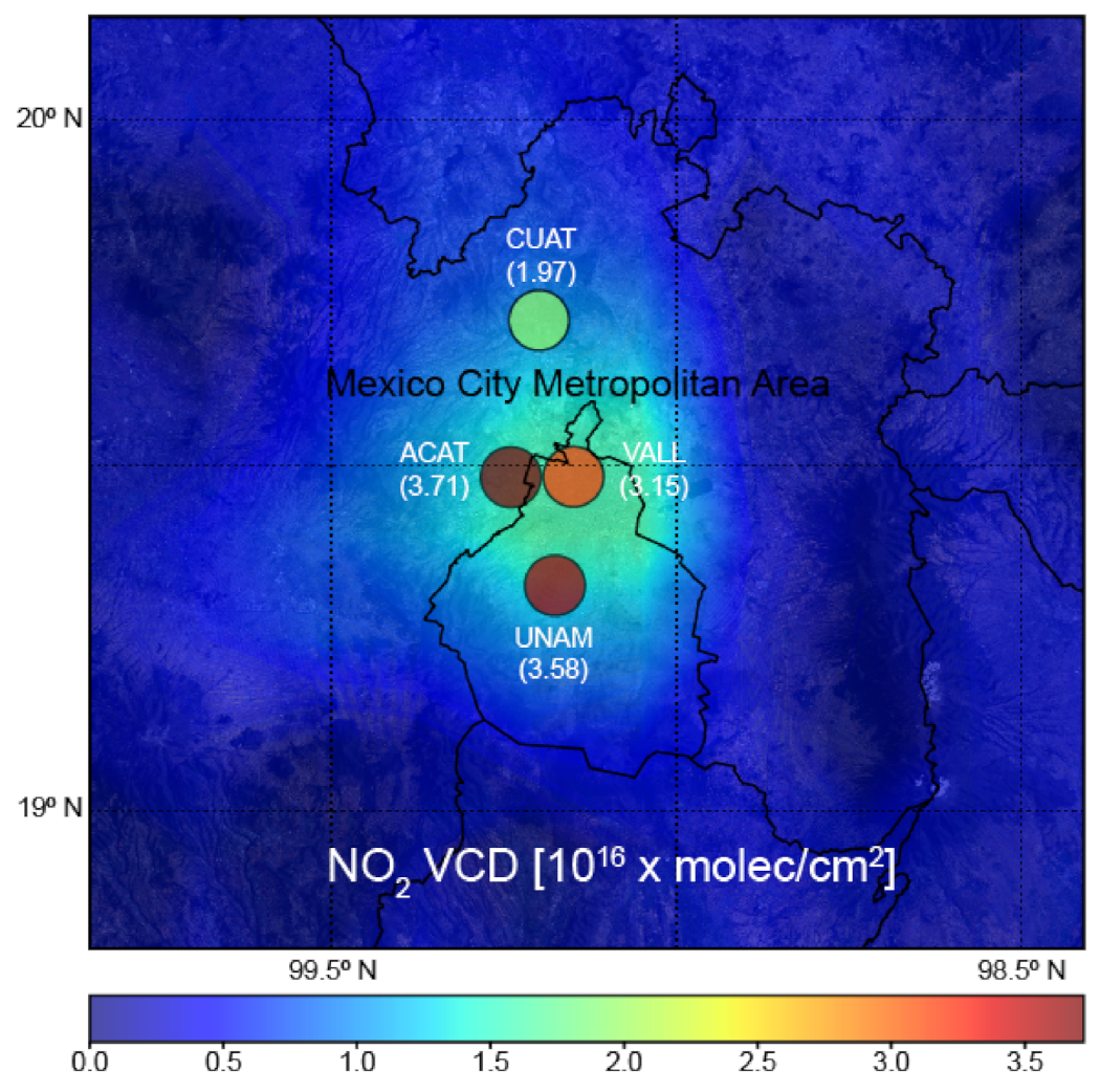
2.2. The MAX-DOAS Network in Mexico City

A MAX-DOAS network was deployed in 2012 to increase the information and knowledge about the trace gases in the tropospheric vertical column within the MCMA [14]. It has been demonstrated that the DOAS technique can provide useful information for the tropospheric observations of trace gases both in large urban regions and remote sites. Each of the four sites operated in the MCMA has its own characteristics from the diverse sources around it and its own variability.

According to the local emissions inventory [12], the NO${}_2$ is strongly associated with vehicular and industrial activities. Typical wind patterns in the region, with a dominant north-to-south flow, are recurrent and are affected by the mountain range that surrounds the basin. A topographical gap on the north where the trade winds penetrate influences the transport and distribution of pollutants [34].

The locations of the four MAX-DOAS instruments that form this small network, were chosen to cover an approximate area of 370 m${}^2$ and a wide range of conditions but also taking advantage of the current infrastructure from UNAM (National Autonomous University of Mexico) and the air quality network run by the city government (SEDEMA). The instrument furthest south (UNAM) is at the central university campus (19.33N, 99.18W), with large complementary measurements performed by the Center of Atmospheric Sciences. Acatlán (ACAT) is also on a university campus located in the highly urbanized western part of the city (19.48N, 99.24W). Vallejo (VALL), at SEDEMA’s central lab for analysis and instrument maintenance (19.48N, 99.15W), is a station that is adjacent to a highly industrialized region within the city. To the north, in the outskirts of the city but next to the highway going to Querétaro, is the Cuautitlán (CUAT) station (19.71N, 99.20W), where SEDEMA operates an air quality monitoring station within a recreational park.

The four instruments have the same construction design and characteristics. They collect scattered solar radiation in the UV/Vis spectral range of 286 to 510 nm, with a telescope that performs multi-angle scans in one particular azimuth direction. Each scanning sequence consists of 36 elevation angles; the first observation is towards the zenith and then completes a full scan from west to east and finishes with the collection of a dark spectrum, with a motorized shutter installed within the scanning unit. An optical fiber directs the collected light from the telescope in the scanning unit to a spectrometer (Ocean Optics, USB2000+), installed within a separate acquisition and control unit located indoors. The spectrometer, temperature regulated to 20 °C with a $\pm 0.5$ °C precision, is connected to a laptop computer for control and acquisition purposes. For a detailed description of the instrument construction and performance, please refer to Arellano et al. (2016) [14].

On a clear day, there are about 150 sequences measured in the period between 7 and 19 h LST, and the instrument operates automatically. Each sequence contains the spectral data at each elevation angle, including the zenith that is used as a reference and a dark spectrum that is subtracted from each spectral measurement to eliminate variations from temperature-dependent instrumental radiances and noise.

QDOAS v2.105 [35], is used to retrieve differential slant column densities (dSCDs) from the measured spectra by fitting absorption cross-sections of the gases and other parameters. For the results shown in this work, O${}_4$ dSCDs were retrieved from the 336–390 nm spectral region using the cross-sections: O${}_4$ [36], O${}_3$ at 221 K and 241 K [37], NO${}_2$ at 294 K [38], BrO at 298 K [39], and HCHO at 298 K [40]. For NO${}_2$ dSCDs, the 405–465 nm region was chosen for the retrievals using the cross-sections: NO${}_2$ at 298 K [38], O${}_3$ at 221 K [37]. The Ring spectrum was adjusted to 273 K from the high-resolution data [41], and a polynomial of degree 3 was used for both species. A nonlinear least square fit adjusted to the solar atlas [41] was applied, solving the logarithmic difference in the intensity of the absorption spectrum.

To have a reference point between retrievals from MMF code using different settings, we made a comparison between the VCDs results from this work and the ones using the retrieval setting used in a project for the TROPOMI instrument validation [42,43]. The dSCDs retrieved in that study used the 338–390 nm window for O${}_4$ and 425–465 nm for NO${}_2$. The comparison was made between December 2017 to April 2018, a period with the highest levels of NO${}_2$. The VCDs from our retrieval settings, used also by Friedrich et al. (2019) [44], were only slightly lower (slope = 0.95) and resulted in a Pearson Correlation of 0.98.

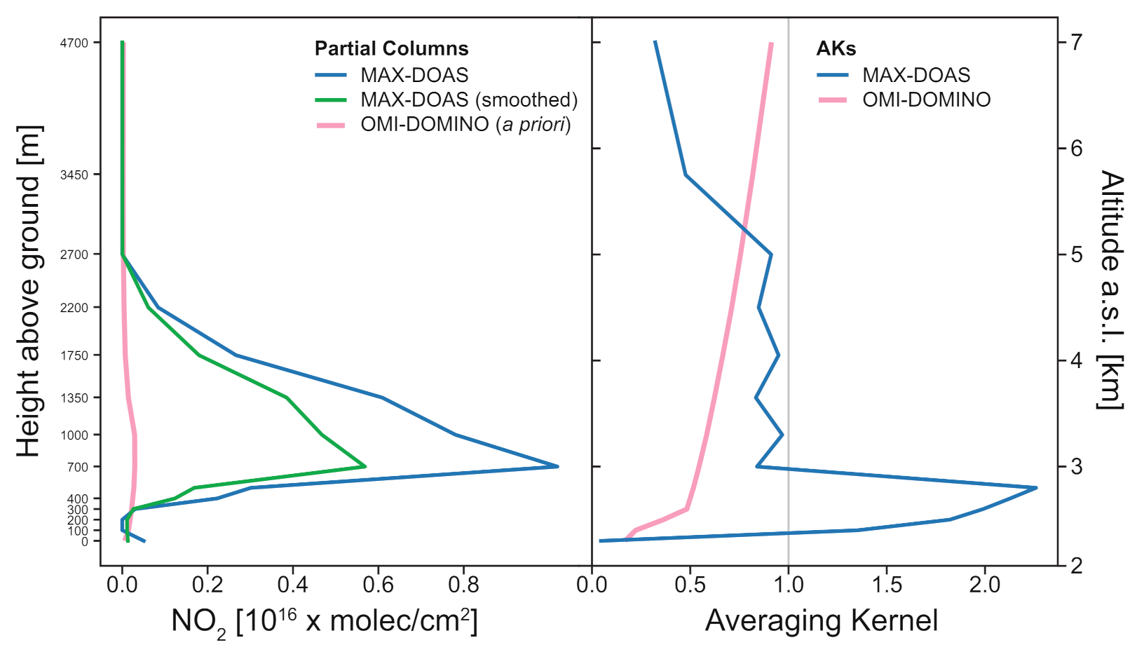
2.3. MMF Retrieval Code

The Mexican Maxdoas Fit (MMF) retrieval code is developed to retrieve trace gas and aerosol concentration profiles, as well as their integrated quantities VCD and AOD, from slant column densities of the trace gas in question and the oxygen dimer O${}_4$ measured at a range of different (low) elevation angles [44]. As many other such retrieval codes, e.g., BePro [45] or HeiPro [46], it works in a two-step process. First the known oxygen dimer O${}_4$ profile is used to retrieve an aerosol profile ingesting the O${}_4$ dSCDs from the QDOAS retrieval and then using the retrieved aerosol profile in the forward model that forms part of the trace gas retrieval ingesting the trace gas (here NO${}_2$) dSCDs from the QDOAS retrieval.

As a forward model, MMF uses VLIDORT v.2.7, developed in Spurr et al. [47,48,49] and for both retrievals (aerosol profile and trace gas), MMF uses a constrained least square fit in the inversion and a Gauss–Newton iteration scheme is used. The aerosol retrieval uses a Tikhonov regularization and an a priori profile shape from hourly averages of one year of ceilometer measurements. For the single scattering albedo and the asymmetry factor, data from the UNAM Aeronet station are interpolated at the measurement time and retrieval wavelength. The trace gas retrieval relies on an optimal estimation approach using a covariance matrix and an a priori profile constructed using the mean and covariances from one year of WRF-Chem v.3.6 model data over Mexico City.

In this investigation, 22 unevenly spaced retrieval layers up to a height of 10 km above ground were used. For more details on MMF as well as specific settings for the retrieval parameters used in this study, we refer the reader to Friedrich et al. (2019) [44], where the algorithm is described in detail and all parameter settings that are not already listed here are provided. MMF has also recently been used in a study about formaldehyde (HCHO) based on spectra from the same instruments [50].

Apart from the profiles and integrated quantities, MMF also outputs averaging kernels and DOF as diagnostic parameters, as well as smoothing error and noise error. Friedrich et al. (2019) [44] performed a detailed investigation of the different error contributions of the trace gas retrieval, however, only for the UNAM station and for a shorter amount of time. The estimated total error on the VCD for that station was found to be around 20% considering all measurements during the day (roughly 7 to 19 h LST). A similar analysis is performed here for all four stations, both using the complete data sets (7–19 h LST) as well as only taking into account measurements at the OMI overpass time (13–15 h LST). The results are summarized in

Table 1. Average errors for the data available for each MAX-DOAS site over the day and the 13–15 h LST period all the data set available for each site.

	UNAM		VALL		ACAT		CUAT
Around Satellite overpass time (13–15 LST)
	molec/cm${}^2$	%	molec/cm${}^2$	%	molec/cm${}^2$	%	molec/cm${}^2$	%
Noise	$3.63\times {10}^{14}$	1.1	$3.85\times {10}^{14}$	1.2	$4.27\times {10}^{14}$	1.15	$5.39\times {10}^{14}$	2.8
Forward	$3.73\times {10}^{15}$	10.4	$4.17\times {10}^{15}$	13.2	$4.90\times {10}^{15}$	13.3	$3.25\times {10}^{15}$	17.7
Smooth	$2.32\times {10}^{15}$	6.5	$2.41\times {10}^{15}$	7.6	$2.53\times {10}^{15}$	6.8	$3.69\times {10}^{15}$	19.5
Parameters	$3.34\times {10}^{15}$	9.4	$1.88\times {10}^{15}$	6.1	$2.0\times {10}^{15}$	5.4	$3.97\times {10}^{15}$	21.2
Total error		15.5		16.5		16.0		34.0
All Day (7–19 LST)
	molec/cm${}^2$	%	molec/cm${}^2$	%	molec/cm${}^2$	%	molec/cm${}^2$	%
Noise	$3.63\times {10}^{14}$	2.4	$4.81\times {10}^{14}$	1.9	$3.97\times {10}^{14}$	1.9	$4.5\times {10}^{14}$	3.0
Forward	$3.73\times {10}^{15}$	12.3	$3.96\times {10}^{15}$	15.5	$3.96\times {10}^{15}$	19.4	$3.96\times {10}^{15}$	26.3
Smooth	$2.32\times {10}^{15}$	12.6	$3.33\times {10}^{15}$	13.0	$2.48\times {10}^{15}$	12.2	$2.91\times {10}^{15}$	19.3
Parameters	$3.34\times {10}^{15}$	9.4	$1.56\times {10}^{15}$	6.1	$1.10\times {10}^{15}$	5.4	$7.79\times {10}^{15}$	51.9
Total error		20.1		21.2		23.6		61.4

.

First retrieval results for the measurements at UNAM site have been presented elsewhere [44] together with the detailed error analysis as suggested by Rodgers [33], which contain further information about the retrieval and error analysis. The error ${ϵ}_{full}$ in the retrieved NO${}_2$ VCD is the difference between the retrieved profile (x) and the true profile ($x_{true}$) and includes also the smoothing error (${ϵ}_{smooth}$) (${ϵ}_{full}$ = ${ϵ}_{smooth}$ + $ϵ$), while the error is the difference between the retrieved and the smoothed true profile described by the following equation [x – $x_{apriori}$ = AK($x_{true}$ – $x_{apriori}$) + $ϵ$]. The right-hand side term is for the smoothed true profile plus the errors related to the forward model, forward model parameter, and the noise error. All errors are shown in Table 1: Noise error (Noise) [$G_{yϵ}$] from the natural measurement errors propagated from the spectral noise, to the slant column densities and finally to the MMF retrieval, the forward model error (Forward) [$G_y\Delta f(x,b,b^{\prime })$] and forward parameter error (Parameter) [$G_{y}Kbf(x,b,b^{\prime })$] and finally the smoothing error (Smooth) [${ϵ}_{smooth}=(AK-I)(x_{true}-x_{apriori})$] describing due to the averaging kernel the limitation of retrieving fine structures in the profile.

For UNAM, VALL, and ACAT, the errors are comparable and are in the same range as found by Friedrich et al. (2019) [44] for the complete UNAM dataset, around 20%. However, for the CUAT station, the estimated total VCD errors are much higher, around 61% and around 34% for the whole data set and restricted to OMI overpass time, respectively. The largest contribution to the higher error for CUAT station comes from the parameter error in the forward model, likely indicating a higher degree of horizontal in-homogeneity (the forward model assumes uniform layers). The effective distance for MAX-DOAS instruments operating in the visible is around 10–20 km, depending on the weather, the solar zenith angle as well as on the details of the aerosol distribution. Since the CUAT station is located in an ecological park with dimensions less than a few hundred meters in an east–west direction and a couple of km in the north–south direction, it is likely that the horizontal distribution is less homogeneous in the area probed by the MAX DOAS instrument.

2.4. Surface Measurements

NO${}_2$ is routinely monitored in the city with in situ analyzers at the surface by the air quality network run by the city government (SEDEMA). This Automatic Network of Atmospheric Monitoring, referred to with the acronym RAMA from its name in Spanish, operates more than 30 stations, distributed within the Mexico City boundaries and in some municipalities of the State of Mexico. RAMA reports hourly data of criteria pollutants like ozone, nitrogen oxides (NO${}_x$ = NO + NO${}_2$), sulphur dioxide, carbon monoxide, and particulate matter that are available for download from their web page [aire.cdmx.gob.mx]. The network uses sampling chemiluminescence analyzers to detect NO${}_x$, based on the emission of light after the NO in the sample being oxidized with excess ozone, and the chemiluminescence is proportional to the NO in the sample.

In addition, a heated (315 ${}^{\circ }$C) molybdenum catalytic converter reduces all the nitrogen oxides to NO allowing for quantifying the NO${}_x$ separately and thus the amount of NO${}_2$ in the sample is estimated from the difference (NO${}_2$ = NO${}_x$ – NO). The four MAX-DOAS instruments are co-located with RAMA stations; however, the Vallejo RAMA station did not operate over the full MAX-DOAS time series. Hence, for a comprehensive comparison over the time series, we use the products of the Camarones station that were taken at less than 3 km from Vallejo (19.28N, 99.11W).

3. Results

In Section 3.1, we present an evaluation of the DOMINO NO${}_2$ product v.2, retrieved from measurements obtained over Mexico City with the OMI instrument on board the Aura satellite, with measurements performed with a network of four MAX-DOAS instruments from the ground. In Section 3.2, the VCD data from the ground-based remote sensing instruments is then compared with 1-hour averages taken from in situ analyzers in order to evaluate the ability of the MAX-DOAS to detect the variability of NO${}_2$ near the surface.

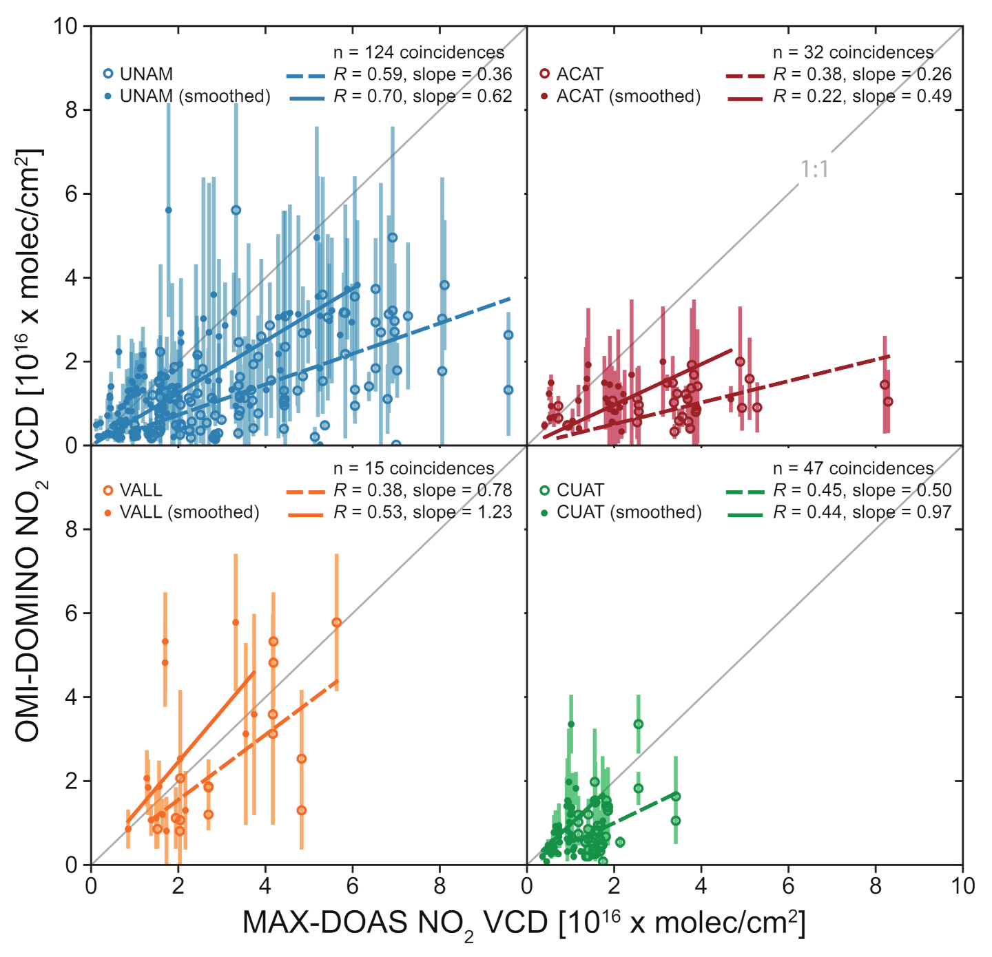
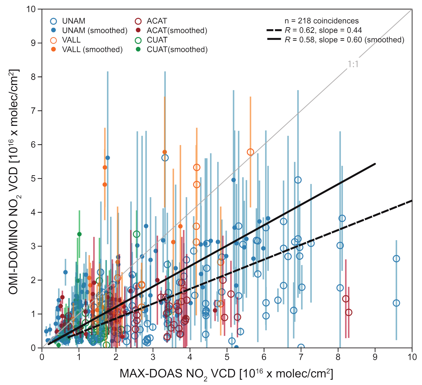
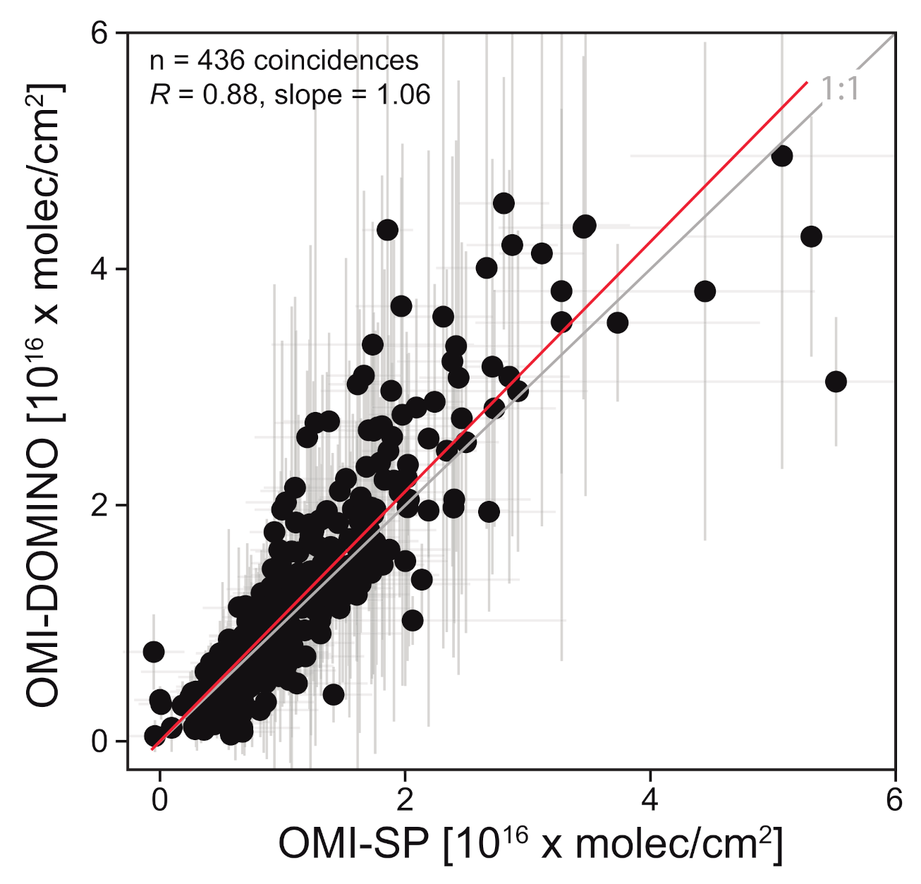
3.1. Comparison with Satellite-Based Measurement

The NO${}_2$ column data collected from the four MAX-DOAS stations, placed such as to achieve a representative coverage of the MCMA, were used to evaluate the DOMINO product from the OMI satellite instrument in a highly polluted environment. VCDs retrieved from the ground-based measurements were compared with those obtained from the space-borne observations taking into account their vertical-dependent sensitivities (AK). During the satellite overpass at around 14:00 h LST, the NO${}_2$ VCD typically decreases, due to its photolysis in the presence of UV radiation, although it may also increase during specific pollution or transport events.

This dynamic behavior and high variability in the NO${}_2$ calls for a short averaging time of the ground-based measurements around the overpass time. However, after applying the DOF and RMS filters, many ground-based measurements are rendered invalid. Hence, we take ground-based data $\pm 30$ min of the overpass time into account in order not to lose too large of a fraction of the data. This choice of averaging time is not unusual in comparisons of ground-based and satellite observations [32].

The OMI data are also filtered for clouds and for a spatial successful coincidence; we selected the nearest valid OMI pixel to the MAX-DOAS station that was within a radius of 15 km (see Section 2.1) The center of the nearest OMI pixels to each MAX-DOAS station was on average around 9 km.

The available MAX-DOAS NO${}_2$ data set comprises 626 total coincidences with OMI (124 after applying OMI filters) for the UNAM site between February 2013 and June 2018, 148 total coincidences (32 after the OMI filtering) for Acatlán between April 2014 and October 2017, 98 total coincidences (47 after OMI filtering) for Cuautitlán in the period between April 2014 to October 2018, and 88 total coincidences (15 after the OMI filtering) for Vallejo between January 2013 and November 2018. In the latter, the dataset consisted of only 15 coincident measurements in the analysis and the results may therefore not be statistically robust.

The OMI DOMINO NO${}_2$ tropospheric VCDs time series during this intercomparison study is shown by pink circles in Figure 1. The presented NO${}_2$ VCDs from OMI are without any filter. All individual NO${}_2$ VCD measurements from each MAX-DOAS station that fall within the period around the overpass time are also shown in the figure: UNAM in blue, Vallejo in orange, Acatlán in red, and Cuautitlán in green. It can be seen that, despite the large data gaps in ground-based data due to diverse maintenance, communication, and operational problems of the MAX-DOAS instruments, we could still gather sufficient information for a proper evaluation of the satellite product and describe the total column NO${}_2$ variability in the region.

It is evident from Figure 1 that the values measured by the ground-based instruments are generally larger than the satellite product. A fit of the OMI-DOMINO data was applied using the Fourier analysis (Equation (2)), from which a clear annual cycle in the VCD over Mexico City is discernible with maxima during the winter (November to February). The fit suggests a slightly decreasing trend ($-0.29\times {10}^{15}$ molec/cm${}^2$ yr) of the NO${}_2$ abundance over this 7-year period.

Figure 2 is a map with the mean spatial distribution of NO${}_2$ above the MCMA reconstructed from all OMI valid measurements between 2013 and 2018. A $10\times 10$ km${}^2$ mesh is covering the domain and all available OMI measurements within a 15 km circle around each grid point are averaged to the VCD. Some measurements are contributing to more than one gridpoint and thus the method is sometimes referred to as an oversampling method. MAX-DOAS data were averaged close to the satellite overpass time (13–15 h LST) with the available measurements. The color of the circles, following the same color scale as the satellite data, corresponds to the average VCDs measured at each station according to the data presented in Figure 1. The radius of each circle is 10 km. This is an approximation of the detection range of the instrument at the surface, which depends on the visibility, the cloudiness, and the height of the mixing layer [14].

Supporting what has been seen in Figure 1, the MAX-DOAS values appear to be almost twice from the OMI VCDs in the central (Acatlán and Vallejo) and southern (UNAM) sites, while the average value registered at Cuautitlán, in a more rural location, is closer to the average column measured by OMI. It is essential to highlight from the map that the higher NO${}_2$ values are centered in the region of the MCMA with the larger population density and traffic flow [12].

Figure 3 shows correlation plots with the Pearson’s correlation coefficients between each of the MAX-DOAS instruments and the OMI-DOMINO NO${}_2$ VCDs for those data pairs complying with the coincidence criteria explained before. MAX-DOAS VCDs are plotted with open circles and those with filled circles are calculated from smoothed profiles using the AK and a priori from the DOMINO product. This procedure is necessary when comparing remote sensing instruments (Section 2) according to Rodgers [16]. We use the DOMINO AK profiles to smooth the MAX-DOAS profile, by interpolating them to the 22 levels in the MMF output.

An example of the smoothing effect is shown in Figure 4 for data from 26 January 2013. In the left plot, the retrieved MAX-DOAS profiles without (blue) and with the applied vertical, smoothing with the AK from OMI (green) are shown, as well as the a priori profiles from OMI (pink). As described above (Equation (2)), the smoothed profile was created using the Rodgers [16] suggestion.

In the right panel of Figure 4 are the AKs from MAX-DOAS and that from the OMI-DOMINO product interpolated to the MAX-DOAS layer scheme.The OMI’s AK profile in this example, and, similarly to that from other days, shows a low surface sensitivity (AK < 0.5) in the first half kilometer above the surface (between 2.3 and 2.8 km a.s.l.), while at higher elevations the AK is steadily increasing from around 0.5 to almost 1. The AK from OMI has a similar shape at most of the days although it is sometimes slightly shifted to larger values (closer to 1.0). By the time of the satellite overpass, the mixing layer is usually in its maximum height, from 10–14 h LST can grow 2 km [51], and it is expected that most of the sensed NO${}_2$ in this polluted environment will be contained in the altitude region where the satellite presents reduced sensitivity. The MAX-DOAS AK in Figure 4 (right plot) shows a different shape. It is less than one near the surface (<100 m) in this example, larger in the first 700 m and then stays close to 1.0 up to 3000 m above ground. Similar results are obtained for different days, although some small features can change depending on the ambient conditions.

In Figure 5, we present the correlations obtained when MAX-DOAS data from all four stations (See Figure 4) are compared together with the closest pixel-measurements from OMI to each of the stations. The data were analyzed without (open circles) and with OMI’s AK smoothing of the MAX-DOAS results (filled circles) and a linear regression of the data-pairs were calculated. No significant change was observed in the overall Pearson’s correlation coefficient ($R\approx 0.6$) after the MAX-DOAS data was smoothed; however, this procedure had a large effect on the slope of the linear fit increasing from 0.44 to 0.60.

From OMI AKs, see the right-hand panel of Figure 4, it is apparent that OMI is not very sensitive to NO${}_2$ in the lowest 1000 m above ground and hence the contribution of these lower layers to the NO${}_2$ VCD measured by OMI is dominated by the a priori (see the left-hand panel for an example of an OMI a priori) used in the OMI product retrieval instead of NO${}_2$ located in those layers. Therefore, it is expected that the slope of the correlation of the linear fit between OMI and MAX-DOAS VCDs increases if the smoothing is taken into account.

The AK of the MAX-DOAS measurements, on the other hand, shows values considerably larger than one at heights around 1 km above the surface and hence results in an overestimation of the true VCD if the boundary layer raises to and above these heights. The mixed layer heights over Mexico City exceeding 2 km was found to be not uncommon during the afternoon [51].

When the stations were compared independently with the satellite product, as one can see in Figure 3, the slopes from the smoothed data sets collected in the three sites situated in highly urbanized neighborhoods, UNAM, Acatlán, and Vallejo were 0.62, 0.49, and 1.23, respectively. The fourth station, with 47 coincidences, is on the outskirts of the city and about 27 km north from the Acatlán and Vallejo central sites. For this site, we obtained a slope of 0.97 after smoothing. The limited correlations found in the individual sites may have to do with the large horizontal inhomogeneity in the NO${}_2$ distribution and the relatively large pixel size of the satellite observation. When the four locations are compared at the same time, the correlation coefficient improves, and we obtain a slope of 0.60 (see Figure 5).

In this investigation, we focus on the comparison with the DOMINO product and not the SP, since the DOMINO online version includes the AK matrix, and both demonstrate to be rather consistent (R = 0.89). Figure 6 shows the comparison between DOMINO (v.2) and the SP (v.3), both are generated from the same measured spectral radiances, but using spectral window between 405–465 nm and 402–465 nm, respectively, to retrieve the dSCDs.

The AMFs from the transport models of each product (Section 2.1) are needed to retrieve the VCDs that simulate the initial NO${}_2$ vertical profile. A study between the two OMI products and in situ measurements of annual NO${}_2$ concentrations in the Southern United States showed a bias for the OMI products of 27–43% for SP (v.1.05) and 21–33% for DOMINO (v.1.02) [52].

According to that study, both products show similar seasonal and spatial variations but have their differences mainly over continental areas. They associate this seasonal difference to the AMF of each product. DOMINO v.2 had a better resolution in the input parameters until an improved SP v.3 was released. We have also compared the ground-based data with SP, and the results are not much different (a difference of around –0.1 from Pearson correlation) than with DOMINO (not smoothed).

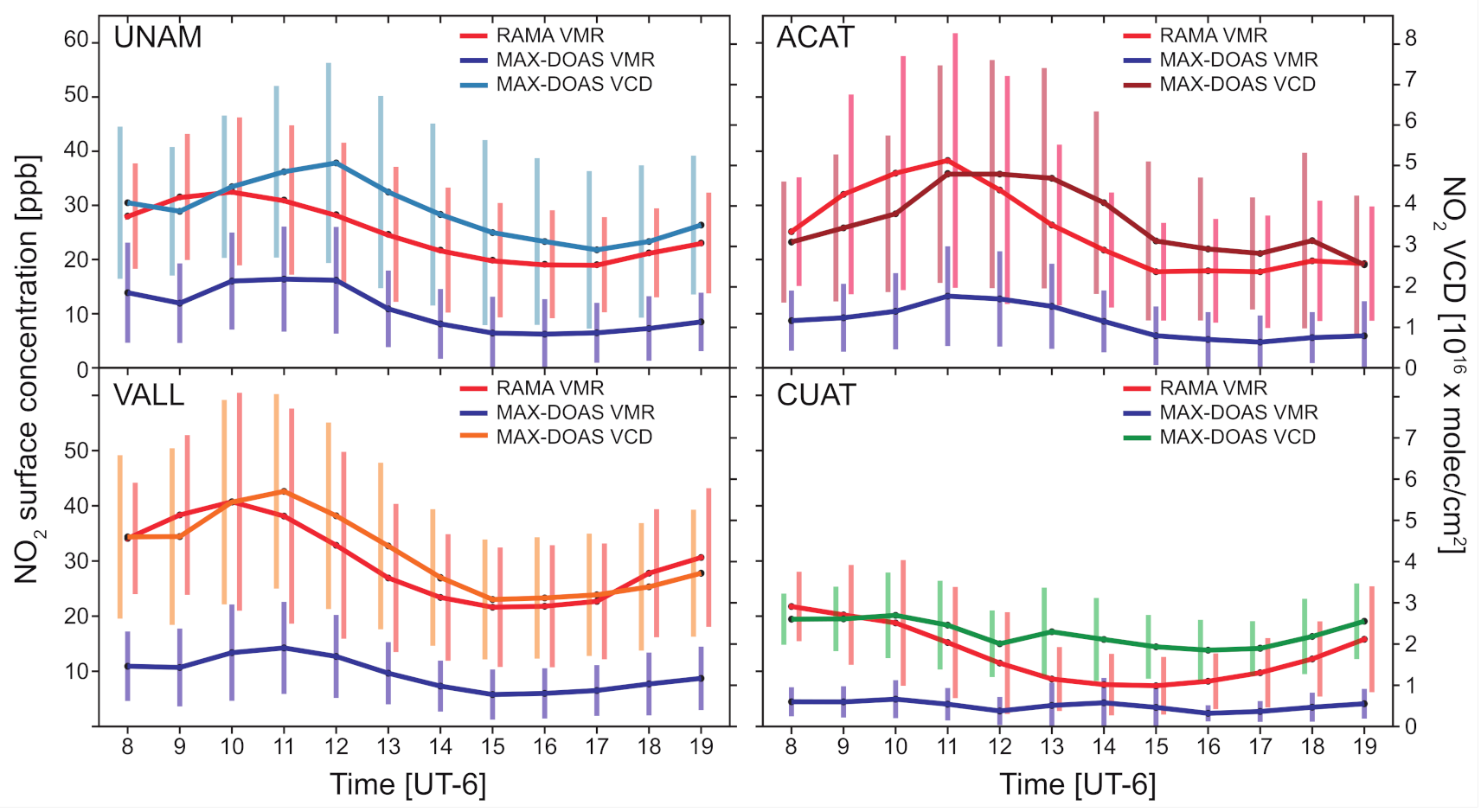
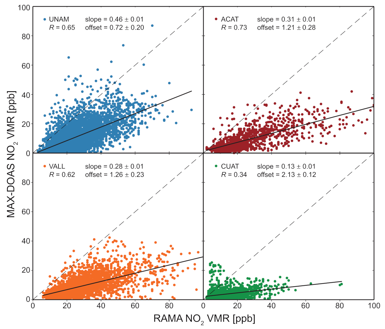
3.2. Comparison with RAMA Measurement

Similar to what has been shown previously for the UNAM site [44], Figure 7 shows the the results of the comparison between MAX-DOAS and surface measurements carried out by in situ gas analyzers run by the air quality monitoring network from the city government. This can be done since all four MAX-DOAS instruments are located in stations from the RAMA air quality network, see Section 2.4. The RAMA data represent the pollution at the surface as opposed to the total vertical column measured by OMI or the MAX DOAS instruments. The colored lines (color code as in Figure 3) in the plots of Figure 7 show the hourly means of the VCDs measured by the MAX-DOAS instruments for the entire period with coincident RAMA data and in red are the mean hourly surface concentrations measured by the corresponding RAMA station (in parts-per-billion units, shown in a different scale).

For the comparison, we take the NO${}_2$ partial columns retrieved from all the MAX-DOAS instruments. We select the first six partial columns above ground, within the first 715 m above the ground (six lowest layers of the MMF output) and averaged to a “superficial column”. These partial columns, with VMR values in ppb, are shown as blue lines in Figure 7. It is apparent from Figure 7 that these average VMR values from the MAX-DOAS profile retrieval follow fairly well the RAMA diurnal cycle; however, the MAX-DOAS values are considerably smaller. This might be explained by the low sensitivity in the lowest layers (see MAX DOAS averaging kernel in the left-hand panel of Figure 4). These and the diurnal cycles were constructed for the days when the MAX-DOAS instrument had coincidences with RAMA.

The NO${}_2$ patterns in Figure 7, as expected from traffic and related anthropic activity, show an increase during the morning hours peaking at around 10 h LST, followed by a decrease until approximately 17 h LST both from a dilution caused by the growing mixing layer and the photochemical activity. During the last two hours before sunset (17–19 h LST), a little increase in NO${}_2$ can be detected and may be attributed to increased emissions during the evening rush hour, when people return from work.

CUAT presents a somewhat different pattern than the other stations, which can in part be explained by the location of the instrument. As seen in Figure 2, the CUAT station is outside the highly urbanized city and installed within an ecological park. The average NO${}_2$ concentrations registered by both measurements are not only lower, but the diurnal pattern also seems to be distinct. The characteristic peak during the morning hours is absent and the relative NO${}_2$ concentration presents a considerable increase in the afternoon. This last feature may be caused by pollution transport events, supported by the peak observed from the column measurement at around 13–15 h LST that is not evident from the measurements at the surface. The error bars in Figure 7 represent the data dispersion from their calculated standard deviations.

We present in Figure 8 the correlation plots of coincident hourly mean data between the surface measurements from RAMA and the MAX-DOAS VMR calculated based on the partial column up to 750 m above ground. The Pearson’s coefficients (R) lie between 0.62 and 0.73 for all three stations in highly urbanized locations, whereas R = 0.34 for Cuautitlán station.

This low correlation is consistent to what can be observed in Figure 7 and may be due to a combination of factors. As we mention above, the CUAT station is located on the outskirts of the city and presents the lowest NO${}_2$ concentrations of all four stations, and the MAX-DOAS may have difficulties in detecting the concentrations measured near the surface. It is also possible that, at this site, polluted air masses that are being transported aloft are detected by the MAX-DOAS instrument and not by the gas analyzer at the surface.

This is supported by a set of data shown in the dispersion plot of CUAT in Figure 8 with larger MAX-DOAS values that were probably not detected by the instrument at the surface. This site also presents the lowest slope in the linear regression (0.13) with respect to the surface measurement, when compared to those obtained for the other stations (0.28–0.46).

4. Conclusions

In the present investigation, we evaluate the OMI-DOMINO NO${}_2$ satellite product with a rich set of ground-based measurements that consist of four MAX-DOAS instruments co-located at surface air quality monitoring stations. The study included strict quality control of the data and the use of coincidence criteria that reduced the number of data pairs considerably, but the six-year period used since the four MAX-DOAS remote sensors were installed within the MCMA between 2013 and 2018, allowed us to perform a robust comparison. In addition, the individual calculation of systematic and random errors of the ground-based measurements, which sum up to around 20%, as well as an in-depth analysis of the retrieval diagnostics provide us with sufficient information to interpret the differences obtained when these remote sensing techniques were compared.

In general, the NO${}_2$ columns retrieved from measurements of the OMI instrument on board the Aura satellite are significantly lower than those retrieved from measurements of MAX-DOAS instruments. A time series showing the data sets from both satellite and ground-based observations makes this evident. However, the plot also reveals that both techniques measure a similar variability throughout the seasons. The slopes obtained from the linear regressions obtained at the UNAM, Acatlán, Vallejo, and Cuautitlán stations were 0.36, 0.26, 0.78, and 0.50, respectively. After smoothing the MAX-DOAS NO${}_2$ profiles with the AKs from the DOMINO product, these slopes increased to 0.62, 0.49, 1.23, and 0.97, respectively. This improvement can be attributed to the low sensitivity of the space borne instrument which is accounted for when smoothing the ground-based measurements with the OMI averaging kernel. An overall slope of 0.44 (0.60 after smoothing) was obtained when the coincident data from all four stations were combined in the regression with a correlation coefficient of R = 0.62, which did not improve after the smoothing was applied.

A map is presented with the average NO${}_2$ vertical column from all satellite observations available within the study period (Figure 2), including those days without MAX-DOAS coincidences. The map corresponds to the relative mean NO${}_2$ columns measured of the coverage area of the four sites with ground-based observations. Although the spatial distribution is highly smoothed, it reflects the abundance of the NO${}_2$ column above the MCMA. The mean NO${}_2$ columns from ground agree with the map, CUAT station is outside the region of maximum abundance, whereas ACAT, UNAM, and VALL, are within the highlighted area and show the higher mean values for the vertical column. This map reflects the mean distribution among the different years and seasons and can change significantly when data are averaged in shorter time periods as has been shown in a previous study [53].

We also present for each station the diurnal variability of the NO${}_2$ columns and compare this to the surface concentrations obtained from in situ instruments. The measurements to an average VMR calculated from the partial column up to 750 m above ground retrieved with the MAX-DOAS instrument are also compared (Figure 8). Here, we obtain good correlations (0.62 < R < 0.73) for the three sites within the more urbanized area. This result is in agreement with previous study using UNAM data only, in which the MAX-DOAS average VMR in the lowest layers (750 m above ground) vs. surface measurement had an R value result of 0.74 and a slope of 0.46 [44]. In Cuautitlán, where the lowest NO${}_2$ abundances are observed, a lower correlation (R = 34) was observed. This is attributed to the location of the station, being such that the transported pollution detected in the column by remote sensing is often not detected near the surface by the in situ instrument. The description of these events where polluted air masses are being transported over a measurement site has been the subject of previous studies [54].

The diurnal cycles of the stations located within the city present maxima at 10–11 h LST, and a decrease in the afternoon due to the NO${}_2$ dilution effect in the mixed layer and various photochemical pathways. It can be noted that, on individual days, different behaviors can be observed depending on the meteorological conditions. These stations present correlation coefficients (0.62 < R < 0.73) revealing that the MAX-DOAS captures the variability rather well. In Cuautitlán, as mentioned above, there are various factors that contribute to a poor correlation with surface measurements (R = 0.34).

Ongoing work involves the comparison of MAX-DOAS total columns with those retrieved from PANDORA instruments that derive the VCDs from direct solar absorption measurements, the evaluation of products produced from other satellite instruments and the use of prolonged time series from satellite products to report the seasonal variability and trends of NO${}_2$ over this and other cities in Mexico. These exercises are important in order to follow in general terms the evolution of air quality in the different urban centers and to assess the effectiveness of possible mitigation strategies implemented by the local governments.

References

1. Crutzen, P.J. The role of NO and NO2 in the chemistry of the troposphere and stratosphere. Ann. Rev. Earth Planet. Sci. 1979, 19, 443–472. [Google Scholar] [CrossRef]
2. Domenech, X. Origen y Destino de los Contaminantes Atmosféricos. In Química Atmosférica, origen y efectos de la contaminación; Ed. Miraguano: Madrid, Spain, 1991; pp. 43–62. [Google Scholar]
3. Wayne, R.P. The Earth’s troposphere. In Chemistry of Atmospheres, and Introduction to the Chemistry of the Atmospheres of Earth, the Planets, and Their Satellites; Oxford University Press: Oxford, UK, 1985. [Google Scholar]
4. United Nations, Department of Economics and Social Affairs, Population Division. The World’s Cities in 2018, Data Booklet; United Nations: New York, NY, USA, 2018. [Google Scholar]
5. INEGI. Instituto Nacional de Estadística y Geografía. Presentación de resultados. Censo de Población y Vivienda 2020. 2020. Available online: https://www.inegi.org.mx/contenidos/programas/ccpv/2020/doc/Censo2020_Principales_resultados_EUM.pdf (accessed on 14 January 2021).
6. Demographia. Demographia World Urban Areas. 16th Annual Edition 2020.06. St. Louis, US 2020. Available online: http://www.demographia.com/db-worldua.pdf (accessed on 13 January 2021).
7. Molina, L.T.; Madronich, S.; Gaffney, J.S.; Apel, E.; de Foy, B.; Fast, J.; Ferrare, R.; Herndon, S.; Jimenez, J.L.; Lamb, B.; et al. An overview of the MILAGRO 2006 Campaign: Mexico City emissions and their transport and transformation. Atmos. Chem. Phys. 2010, 10, 8697–8760. [Google Scholar] [CrossRef] [Green Version]
8. Solana, O. SEDATU: Secretaría de Desarrollo Agrario y Territorial y Urbano. Anatomy of Mobility in Mexico; Tinta, R., Ed.; The University of Manchester: Manchester, UK, 2018. [Google Scholar]
9. INEGI. Instituto Nacional de Estadística y Geografía. Censo de Población y Vivienda 2020. 2021. Available online: https://www.inegi.org.mx/temas/vehiculos/ (accessed on 13 January 2021).
10. TomTom, Traffic Index Ranks Urban Congestion WorldWide. Available online: https://www.tomtom.com/en_gb/traffic-index/mexico-city-traffic (accessed on 1 December 2020).
11. Belzowski, B.M.; Ekstrom, A. Stuck in Traffic: Analyzing Real Time Traffic Capabilities of Personal Navigation Devices and Traffic Phone Applications; University of Michigan, Transportation Research Institute: Ann Arbor, MI, USA, 2013. [Google Scholar]
12. SEDEMA, Secretaría de Medio Ambiente del Gobierno de la Ciudad de México. Inventario de Emisiones de la CDMX 2016. Dirección General de Gestión de Calidad del Aire, Dirección de Programas de Calidad del Aire e Inventario de Emisiones, Ciudad de México 2018. Available online: http://www.aire.cdmx.gob.mx/descargas/publicaciones/flippingbook/inventario-emisiones-2016/mobile/ (accessed on 12 May 2020).
13. Boersma, K.F.; Eskes, H.J.; Dirksen, R.J.; van der A, R.J.; Veefkind, J.P.; Stammes, P.; Huijnen, V.; Kleipool, Q.L.; Sneep, M.; Claas, J.; et al. An improved retrieval of tropospheric NO2 columns from the Ozone Monitoring Instrument. Atmos. Meas. Tech. 2017, 4, 1905–1928. [Google Scholar] [CrossRef] [Green Version]
14. Arellano, J.; Kruger, A.; Rivera, C.; Stremme, W.; Friedrich, M.; Bezanilla, A.; Grutter, M. The MAX-DOAS network in Mexico City to measure atmospheric pollutants. AMT 2016, 10, 157–167. [Google Scholar]
15. Verhoelst, T.; Compernolle, S.; Pinardi, G.; Lambert, J.-C.; Eskes, H.J.; Eichmann, K.-U.; Fjæraa, A.M.; Granville, J.; Niemeijer, S.; Cede, A.; et al. Ground-based validation of the Copernicus Sentinel-5p TROPOMI NO2 measurements with the NDACC ZSL-DOAS, MAX-DOAS and Pandonia global networks. Atmos. Meas. Tech. 2020, 17, 2189–2215. [Google Scholar]
16. Rodgers, C. Intercomparison of remote sounding instrument. J. Geoph. Res. 2003, 108. [Google Scholar] [CrossRef] [Green Version]
17. Baylon, J.L.; Stremme, W.; Grutter, M.; Hase, F.; Blumenstock, T. Background CO2 levels and error analysis from ground-based solar absorption IR measurements in central Mexico. Atmos. Meas. Tech. 2017, 10, 2425–2434. [Google Scholar] [CrossRef] [Green Version]
18. Krotkov, N.; Lamsal, L.; Celarier, E.; Swartz, W.; Marchenko, S.; Bucsela, E.; Chan, K.; Wening, M.; Zara, M. The version 3 OMI NO2 standard product. Atmos. Meas. Tech. 2017, 10, 3113–3149. [Google Scholar] [CrossRef] [Green Version]
19. Hains, J.C.; Boersma, K.F.; Kroon, M.W.; Dirksen, R.J.; Cohen, R.C.; Perring, A.E.; Bucsela, E.; Volten, V.; Swart, D.; Richter, A.; et al. Testing and improving OMI DOMINO tropospheric NO2 using observations from the DANDELIONS and INTEX-B validation campaigns. J. Geophys. Res. 2010, 115. [Google Scholar] [CrossRef]
20. Strahan, S.E.; Duncan, B.N.; Hoor, P. Observationally derived transport diagnostics for the lowermost stratosphere and their application to the GMI chemistry and transport model. Atmos. Chem. Phys. 2007, 7, 2435–2445. [Google Scholar] [CrossRef] [Green Version]
21. Bucsela, E.J.; Celarier, E.A.; Gleason, J.L.; Krotkov, N.A.; Lamsal, L.N.; Marchenko, S.V.; Swartz, W. OMINO2 README Document. Data Product Version 3.0; Tech. Rep. NASA; Goddard Space Flight Center: Greenbelt, MD, USA, 2016. [Google Scholar]
22. Lamsal, L.N.; Krotkov, N.A.; Celarier, E.A.; Swartz, W.H.; Pickering, K.E.; Bucsela, E.J.; Gleason, J.F.; Martin, R.V.; Philip, S.; Irie, H.; et al. Evaluation of OMI operational standard NO2 column retrievals using in situ and surface-based NO2 observations. Atmos. Chem. Phys. 2014, 14, 11587–11609. [Google Scholar] [CrossRef] [Green Version]
23. Chin, M.; Diehl, T.; Tan, Q.; Prospero, J.M.; Kahn, R.A.; Remer, L.A.; Yu, H.; Sayer, A.M.; Bian, H.; Geogdzhayev, I.V.; et al. Multi-decadal aerosol variations from 1980 to 2009: A perspective from observations and a global model. Atmos. Chem. Phys. 2014, 14, 3657–3690. [Google Scholar] [CrossRef] [Green Version]
24. Boersma, K.F.; Braak, R.; Van der A, R.J. Dutch OMI NO2 (DOMINO) Data Product v2.0, HE5 Data File User Manual; Royal Netherlands Meteorological Institute (KNMI): De Bilt, The Netherlands, 2011. [Google Scholar]
25. Huijnen, V.; Williams, J.; Van Weele, M.; Noije, T.; Krol, M.; Dentener, F.; Segers, A.J.; Houweling, S.; Peters, W.; Laat, A.T.J.; et al. The global chemistry transport model TM5: Description and evaluation of the tropospheric chemistry version 3.0. Geosci. Model Dev. Discuss. 2008, 3, 445–473. [Google Scholar] [CrossRef] [Green Version]
26. Platt, U.; Stutz, J. Differential Absorption Spectroscopy; Springer: Berlin/Heidelberg, Germany, 2008; pp. 135–174. [Google Scholar]
27. Bucsela, E.J.; Celarier, E.A.; Wenig, M.O.; Gleason, J.F.; Veefkind, J.P.; Boersma, K.F.; Brinksma, E.J. Algorithm for NO2 vertical column retrieval from the Ozone Monitoring Instrument. IEEE Trans. Geosci. Remote Sens. 2006, 44, 1245–1258. [Google Scholar] [CrossRef]
28. Chan, K.L.; Wang, Z.; Ding, A.; Heue, K.-P.; Shen, Y.; Wang, J.; Zhang, F.; Shi, Y.; Hao, N.; Wenig, M. MAX-DOAS measurements of tropospheric NO2 and HCHO in Nanjing and a comparison to ozone monitoring instrument observations. Atmos. Chem. Phys. 2019, 19, 10051–10071. [Google Scholar] [CrossRef] [Green Version]
29. Wang, Y.; Lampel, J.; Xie, P.; Beirle, S.; Li, A.; Wu, D.; Wagner, T. Ground-based MAX-DOAS observations of tropospheric aerosols, NO2, SO2 and HCHO in Wuxi, China, from 2011 to 2014. Atmos. Chem. Phys. 2017, 17, 2189–2215. [Google Scholar] [CrossRef] [Green Version]
30. Shaiganfar, R.; Beirle, S.; Petetin, H.; Zhang, Q.; Beekmann, M.; Wagner, T. New concepts for the comparison of tropospheric NO2 column densities derived from car-MAX-DOAS observations, OMI satellite observations and the regional model CHIMERE during two MEGAPOLI campaigns in Paris 2009/10. Atmos. Meas. Tech. 2015, 8, 2827–2852. [Google Scholar] [CrossRef] [Green Version]
31. Kanaya, Y.; Irie, H.; Takashima, H.; Iwabuchi, H.; Akimoto, H.; Sudo, K.; Gu, M.; Chong, J.; Kim, Y.J.; Lee, H.; et al. Long-term MAX-DOAS network observations of NO2 in Russia and Asia (MADRAS) during the period 2007–2012: Instrumentation, elucidation of climatology, and comparisons with OMI satellite observations and global model simulations. Atmos. Chem. Phys. 2014, 14, 7909–7927. [Google Scholar] [CrossRef] [Green Version]
32. Pinardi, G.; Van Roozendael, M.; Hendrick, F.; Theys, N.; Abuhassan, N.; Bais, A.; Boersma, F.; Cede, A.; Chong, J.; Donner, S.; et al. Validation of tropospheric NO2 column measurements of GOME-2A and OMI using MAX-DOAS and direct sun network observations. Atmos. Meas. Tech. Discuss. 2020, 76. [Google Scholar] [CrossRef] [Green Version]
33. Rodgers, C. Error Analysis and Characterisation. In Inverse Methods for Atmospheric Sounding. Theory and Practice; World Scientific Publishing Co.: Oxford, UK, 2000; pp. 43–61. [Google Scholar]
34. Salcido, A.; Carreon, S.; Georgiadis, T.; Celada, A.; Castro, T. Lattice wind description and characterization of Mexico City local wind events in the 2001–2006 period. Climate 2015, 3, 542–562. [Google Scholar] [CrossRef] [Green Version]
35. Danckert, T.; Fayt, C.; Van Roozendael, M.; De Smedt, I.; Letocart, V.; Merlaud, A.; Pinardi, G. QDOAS Software User Manual; Belgian Institute for Space Aeronomy Uccle: Brussels, Belgium, 2013; p. 117. [Google Scholar]
36. Hermans, C.A.C.; Vandaele, M.; Carleer, S.; Fally, R.; Colin, A.; Jenouvrier, B.; Coquart, M.F.M. Absorption cross-sections of atmospheric constituents: NO2, O2, and H2O. Environ. Sci. Pollut. Res. 1999, 6, 151–158. [Google Scholar] [CrossRef] [PubMed] [Green Version]
37. Burrows, J.P.; Richter, A.; Dehn, A.; Deters, B.; Himmelmann, S.; Voigt, S.; Orphal, J. Atmospheric remote sensing reference data from GOME-2. temperature dependent absorption cross sections of O3 in the 231–794 nm range. J. Quant. Spectrosc. Radiat. 1999, 61, 509–517. [Google Scholar] [CrossRef]
38. Vandaele, A.C.; Hermans, C.; Simon, P.C.; Carleer, M.; Colin, R.; Fally, S.; Merienne, M.F.; Jenouvrier, A.; Coquart, B. Measurements of the NO2 absorption cross-section from 42,000 cm−1 to 10,000 cm−1 (238–1000 nm) at 220 K and 294 KJ. Quant. Spectrosc. Radiat. 1998, 59, 171–184. [Google Scholar] [CrossRef] [Green Version]
39. Wilmouth, D.M.; Hanisco, T.F.; Donahue, N.M.; Anderson, J.G. Fourier transform ultraviolet spectroscopy of the A 2Π3/2← X 2Π3/2 transition of BrO. J. Phys. Chem. A 1999, 103, 8935–8945. [Google Scholar] [CrossRef]
40. Meller, R.; Moortgat, G.K. Temperature dependence of the absorption cross sections of formaldehyde between 223 K and 323 K in the wavelength range 225–375 nm. J. Geophys. Res. 2000, 105, 7089–7101. [Google Scholar] [CrossRef]
41. Kurucz, R.L.; Furenlid, I.; Brault, J.; Testerman, L. Solar flux atlas from 296 to 1300 nm. Nat. Sol. Obs. Atlas 1984, 1, 337–354. [Google Scholar]
42. Compernolle, S.; Verhoelst, T.; Pinardi, G.; Granville, J.; Lambert, J.C. S5P MPC VDAF Validation Web Article: Nitrogen Dioxide Column Data. Available online: https://mpc-vdaf.tropomi.eu/ProjectDir/reports//pdf/S5P-MPC-VDAF-WVA-L2_NO2_20180904.pdf (accessed on 12 January 2021).
43. Fehr, T. Sentinel-5 Precursor. Scientific Validation Implementation Plan; EOP-SM/2993/TF-tf; European Space Agency: Paris, France, 2016. [Google Scholar] [CrossRef]
44. Friedrich, M.M.; Rivera, C.; Stremme, W.; Ojeda, Z.; Arellano, J.; Bezanilla, A.; García-Reynoso, J.A.; Grutter, M. NO2 vertical profiles and column densities from MAX-DOAS measurements in Mexico City. Atmos. Meas. Tech. 2019, 12, 2545–2565. [Google Scholar] [CrossRef] [Green Version]
45. Clémer, K.; Van Roozendael, M.; Fayt, C.; Hendrick, F.; Hermans, C.; Pinardi, G.; Spurr, R.; Wang, P.; De Mazière, M. Multiple wavelength retrieval of tropospheric aerosol optical properties from MAXDOAS measurements in Beijing. Atmos. Meas. Tech. 2010, 3, 863–878. [Google Scholar] [CrossRef] [Green Version]
46. Frieß, U.; Beirle, S.; Alvarado Bonilla, L.; Bösch, T.; Friedrich, M.M.; Hendrick, F.; Piters, A.; Richter, A.; van Roozendael, M.; Rozanov, V.V.; et al. Intercomparison of MAX-DOAS vertical profile retrieval algorithms: Studies using synthetic data. Atmos. Meas. Tech. 2019, 12, 2155–2181. [Google Scholar] [CrossRef] [Green Version]
47. Spurr, R.J.D.; Kurosu, T.P.; Chance, K.V. A linearized discrete ordinate radiative transfer model for atmospheric remote-sensing retrieval. J. Quant. Spectrosc. Radiat. 2001, 68, 689–735. [Google Scholar] [CrossRef]
48. Spurr, R.J.D. A linearized pseudo-spherical vector discrete ordinate radiative transfer code for forward model and retrieval studies in multilayer multiple scattering media. J. Quant. Spectrosc. Radiat. 2006, 102, 316–342. [Google Scholar] [CrossRef]
49. Spurr, R.J.D. User’s Guide VLIDORT Version 2.6; RT Solutions, Inc.: Cambridge, MA, USA, 2013. [Google Scholar]
50. Rivera, C.; Guarín, C.; Stremme, W.; Friedrich, M.; Bezanilla, A.; Rivera, D.; Mendoza, C.; Grutter, M.; Blumenstock, T.; Hase, F. Formaldehyde total column densities over Mexico City: Comparison between MAX-DOAS and solar absorption FTIR measurements. Atmos. Meas. Tech. Discuss. 2020, 208, 1–27. [Google Scholar]
51. García-Franco, J.L.; Stremme, W.; Bezanilla, A.; Ruiz-Angulo, A.; Grutter, M. Variability of the Mixed-Layer Height Over Mexico City. Bound.-Layer Meteorol. 2018, 167, 493–507. [Google Scholar] [CrossRef]
52. Lamsal, L.; Martin, R.; Donkelaar, A.; Celarier, E.; Bucsela, E.; Boersma, K.; Dirksen, R.; Luo, C.; Wang, Y. Indirect validation of tropospheric nitrogen dioxide retrieved from the OMI satellite instrument: Insight into the seasonal variation of nitrogen oxides at northern midlatitudes. J. Geophys. Res. 2010, 115. [Google Scholar] [CrossRef]
53. Rivera, C.; Stremme, W.; Grutter, M. Nitrogen dioxide DOAS measurements from ground and space: Comparison of zenith scattered sunlight ground-based measurements and OMI data in Central Mexico. Atmosfera 2013, 26, 401–414. [Google Scholar] [CrossRef] [Green Version]
54. Melamed, M.L.; Basaldud, R.; Steinbrecher, R.; Emeis, S.; Ruíz-Suárez, L.G.; Grutter, M. Detection of pollution transport events southeast of Mexico City using ground-based visible spectroscopy measurements of nitrogen dioxide. Atmos. Chem. Phys. 2009, 9, 4827–4840. [Google Scholar] [CrossRef] [Green Version]
Figure 1. NO 2 vertical column densities of the OMI–DOMINO product between 2013 and 2018 (pink) and those from the MAX-DOAS instruments measured close to the overpass time ≈14:00 h LST during the same period (UNAM/blue, VALL/orange, ACAT/red, CUAT/green).
Remotesensing 13 00761 g001
Figure 2. Spatial distribution of the NO 2 VCD monthly averages from the OMI-DOMINO product during the 2013 to 2018 period, together with the overall overpass-time averages from the MAX-DOAS instruments (colored circles) over the MCMA (UNAM: 2013–2018, ACAT: 2015–2017, VALL: 2015–2018, CUAT: 2014–2018).
Remotesensing 13 00761 g002
Figure 3. Correlation plots with coincident data pairs from OMI-DOMINO and each MAX-DOAS instrument in the MCMA taken between 2013 and 2018. Offsets forced to zero, with and without AK smoothing, are shown for UNAM (blue), Vallejo (orange), Acatlán (red), and Cuautitlán (green).
Remotesensing 13 00761 g003
Figure 4. Left: Example of a MAX-DOAS NO 2 retrieved profile from 26 January 2013 (13:55 h LST) without (blue) and with smoothing with the AK from OMI (green). The OMI a priori profile is shown in pink. Right: Averaging Kernels from the OMI-DOMINO (pink) and MAX-DOAS (blue) products. The NO 2 Trop. VCD for this day in molec/cm 2 : MAX-DOAS 8.39 × 10 16 , MAX-DOAS smoothed 3.74 × 10 16 and DOMINO 3.55 × 10 16 .
Remotesensing 13 00761 g004
Figure 5. Correlation plots with coincident data pairs from OMI-DOMINO and all four MAX-DOAS instruments combined. Open circles correspond to the retrievals without any correction and the filled circles are smoothed with the satellite AK. Offsets forced to zero obtained with linear regressions of both data sets are shown with dashed and continuous lines, respectively.
Remotesensing 13 00761 g005
Figure 6. Correlation between the DOMINO (v2) vs the Standard Product (v3) from OMI NO 2 . Linear regression in red and error bars from each data product are shown in grey.
Remotesensing 13 00761 g006
Figure 7. Diurnal cycle over the in situ RAMA network and the superficial column measurements from MAX-DOAS (Up-left) UNAM (Up-right) Acatlán (Down-left) Vallejo and (Down-right) Cuautitlán.
Remotesensing 13 00761 g007
Figure 8. Dispersion plot with coincident hourly means between surface measurements and the average VMR from MAX-DOAS.
Remotesensing 13 00761 g008