Digital Mapping of Soil Organic Carbon Using Sentinel Series Data: A Case Study of the Ebinur Lake Watershed in Xinjiang

Abstract

As an important evaluation index of soil quality, soil organic carbon (SOC) plays an important role in soil health, ecological security, soil material cycle and global climate cycle. The use of multi-source remote sensing on soil organic carbon distribution has a certain auxiliary effect on the study of soil organic carbon storage and the regional ecological cycle. However, the study on SOC distribution in Ebinur Lake Basin in arid and semi-arid regions is limited to the mapping of measured data, and the soil mapping of SOC using remote sensing data needs to be studied. Whether different machine learning methods can improve prediction accuracy in mapping process is less studied in arid areas. Based on that, combined with the proposed problems, this study selected the typical area of the Ebinur Lake Basin in the arid region as the study area, took the sentinel data as the main data source, and used the Sentinel-1A (radar data), the Sentinel-2A and the Sentinel-3A (multispectral data), combined with 16 kinds of DEM derivatives and climate data (annual average temperature MAT, annual average precipitation MAP) as analysis. The five different types of data are reconstructed by spatial data and divided into four spatial resolutions (10, 100, 300, and 500 m). Seven models are constructed and predicted by machine learning methods RF and Cubist. The results show that the prediction accuracy of RF model is better than that of Cubist model, indicating that RF model is more suitable for small areas in arid areas. Among the three data sources, Sentinel-1A has the highest SOC prediction accuracy of 0.391 at 10 m resolution under the RF model. The results of the importance of environmental variables show that the importance of Flow Accumulation is higher in the RF model and the importance of SLOP in the DEM derivative is higher in the Cubist model. In the prediction results, SOC is mainly distributed in oasis and regions with more human activities, while SOC is less distributed in other regions. This study provides a certain reference value for the prediction of small-scale soil organic carbon spatial distribution by means of remote sensing and environmental factors.

1. Introduction

Soil organic carbon (SOC), as the main carbon pool on the land surface, plays an important role in the interactive process of carbon cycle in long time series [1]. Natural and anthropogenic factors within a small area can directly cause changes in SOC and also indirectly affect changes in the carbon cycle within the area [2]. Small changes in SOC can cause changes in atmospheric CO₂ and thus affect a series of global climate changes [3]. Global climate change is a serious problem that threatens the security of Earth’s system and human health today [4]. In order to predict climate change in advance and to find more effective ways to control the direction of climate change, research on the prediction of land surface SOC that causes climate change is an essential step. Soil digital mapping and prediction of soil organic carbon is very important to provide a basis for the whole terrestrial carbon cycle ecosystem and future climate change. Based on this, we have a more comprehensive mapping of soil organic carbon, a more comprehensive understanding of soil carbon storage, but also to promote the global carbon cycle and carbon economy to bring some effect [5].

In the sampling and measurement process of soil organic carbon extraction, the traditional method will spend a lot of manpower and material resources, and through a series of traditional calculation methods [6,7], the accurate distribution of soil organic carbon in a wide range can be obtained [8]. With the wide application of soil digital mapping (SDM), a fast and accurate method for mapping can be provided on the basis of data mining [9]. This method has been widely applied to other soil properties [10]. Applying this method to the monitoring of soil organic carbon greatly improves the efficiency of mapping and monitoring, thus providing a method to reduce the cost of sampling and analysis [11]. The influence of environmental variables on soil properties is not considered in traditional soil mapping. This is the traditional method that only considers soil properties but does not take into account the influence of different climate, topography and other factors on soil properties [12,13]. The selection of environmental covariates can directly affect the distribution of soil organic carbon [14,15]. In a certain area, the change of soil organic carbon is affected by topography, climate, land use, vegetation cover and soil parent material [16]. Temperature and precipitation are highly important climatic factors in the prediction of soil carbon content [17,18]. Terrain attributes are also used as the main predictors of soil organic carbon to study mapping. With the change of terrain attributes, a series of changes will occur in the prediction results and the importance of variables. The importance of selecting covariates is also an essential part of soil organic carbon mapping. Xinjiang is located in arid areas, the distribution of precipitation is uneven [19], climate extremes and terrain fluctuations are obvious [20,21]. Climate and terrain environmental factors have a great impact on the distribution of soil organic carbon, and have a certain leading role in the spatial distribution of SOC.

In the development process of soil mapping, with the development of remote sensing technology and spatial information technology, it has experienced a rapid development process from the initial prediction of distribution through a simple regression model [9,22,23] to the analysis of spatial difference [24,25] to the current digital spatial mapping through machine learning [26,27]. In the development of digital mapping technology, machine learning is a common mapping method. The common methods are RF, Cubist, SVM, BRT, etc. Each method has its own shortcomings, and the appropriate model is selected according to the size of different regions [11,28,29].

With the continuous progress of optical sensors, from the nearest and widely used Landsat series to the Sentinel series [30,31], the spectral resolution is increasing, and the available information is also increasing. The properties and optical characteristics of monitoring surface soil data are continuously improving [32]. In order to ensure the formation of a long-term global earth observation system, the European Space Agency (ESA) has formulated the Sentinel Series Satellite Program. Sentinel-1A Earth observation satellite (SAR satellite) was launched in 2014, Sentinel-2A high resolution multispectral imaging satellite and Sentinel-3A environmental monitoring satellite, were continuously launched from 2015 to 2016 and provided free data [33]. Sentinel-1A data, mainly through their penetration characteristics of soil organic carbon detection, were effective; Sentinels-2A and 3A, through time complementary revisit cycle [34,35] and the combination of different spatial resolutions from high to low at the same time, have many advantages in mapping (fast, time saving, large coverage area, etc.) [36]. The combination of the three not only avoids the error caused by time, but also combines SAR data with spectral data for high-precision multi-time relative SOC prediction, which improves the prediction accuracy and ability. Nowadays, different remote sensing satellites have been launched one after another, and there are many data detected by different sensors. To combine so many sensor data require the use of multi-scale data for soil mapping [37,38]. In different scales, by discussing the selection of optimal scale data for different research areas, the scale selection is used to improve the mapping accuracy to a better level [39,40].

Most soil mapping studies mainly investigate the distribution of soil properties by one kind of satellite data [41,42,43], which weakens the excellent effect of different kinds of satellite data on the extraction of surface parameters. There are some studies to obtain certain results on the distribution and content of surface SOC by Sentinel-1A, Sentinel-2A, and Sentinel-3A data, respectively [30,44], which are limited to one and two kinds of satellite data for analysis during the study [45,46,47], and there are fewer studies to combine the three kinds of data. Meanwhile, the differences of different satellite data at different scales also affect the accuracy of SOC prediction [48]. Therefore, the spatial variation of SOC under different satellite data and different scales needs to be considered comprehensively.

The main purpose of this study is to use two machine learning methods (RF, Cubist) to comprehensively analyze the spatial digital mapping ability of three sentinel sensors (S-1, S-2, S-3) to predict SOC in typical arid areas under two environmental variables (DEM derivatives, climate data), especially under three different types of remote sensing data. At the same time, four spatial resolutions (10, 100, 300, and 500 m) are used to create the SOC prediction model to compare and analyze the prediction effect of different spatial resolution data. The importance of the selected environmental variables was evaluated, and the potential of SOC prediction ability under different environmental variables and different spatial resolution was explored.

2. Materials and Methods

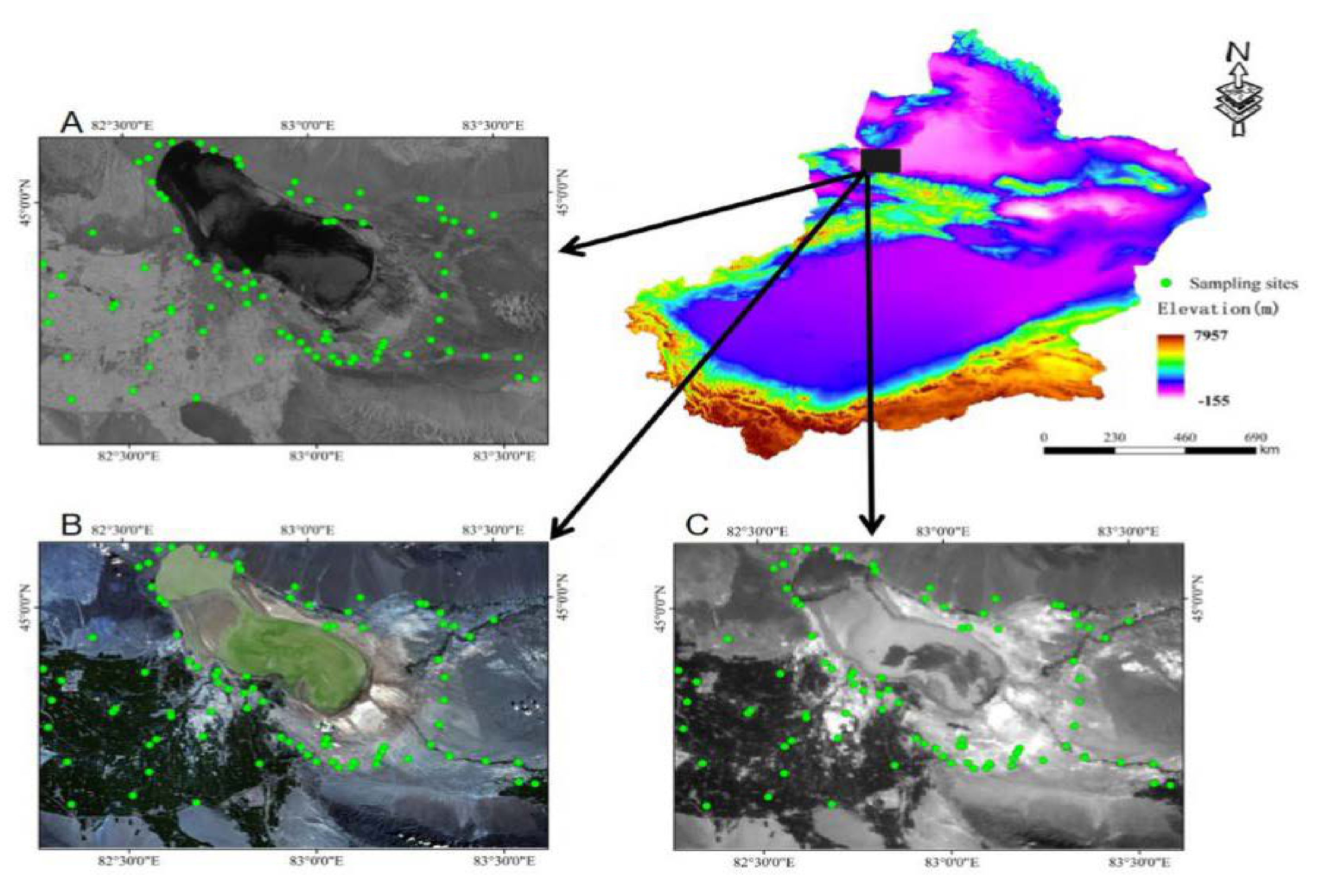
2.1. Study Area

Ebinur Lake Basin is located in the hinterland of Eurasia, and is located in Bortala Mongolian Autonomous Prefecture, Xinjiang, China (44°2′N–45°23′N, 79°53′E–83°53′E) (Figure 1). The elevation difference in the basin is large (4713 m), and the terrain of Ebinur Lake is the lowest. The north–south elevation increases in turn to form a mountain environment. The south is the west edge of Tianshan Mountains, and the east has the largest wind outlet in Asia, Alashankou, forming an extreme terrain environment of wind funnel shape [49]. Affected by the temperate continental arid climate and regional topography, the regional annual average temperature (MAT) was 8.0 °C, the annual average precipitation (MAP) was 89.9–169.7 mm, and the annual average sunshine duration was 2696 h [50]. Due to the strong evaporation in arid areas reaching 1500–2000 mm, the soil level has obvious changes in dry and wet seasons [51,52]. The main types of soil are black calcium soil, chestnut soil, brown desert soil, gray desert soil and gray calcium soil in arid areas. With the change of climate and hydrothermal conditions, SOC has the highest correlation with saline soils, which increases with the increase of soil salinization. In contrast, SOC correlates less with gray-brown desert soils and wind-sanded soils in deserts. Since the study area is located in an arid zone, there is a clear correlation between the change of SOC and the management of soil salinization in the arid zone, thus making the SOC distribution in the area have a certain regional distribution status.

2.2. Soil Data Source

Soil data from the team field sampling data include different land use types and different soil texture surface data (0–10 cm). There were 105 samples in total. After the data were brought back to the laboratory for pretreatment and soil organic carbon experiment, the experiment mainly includes: (1) pre-consolidation of soil—the field sampling soil data were brought back to the laboratory, and the soil was naturally dried in a cool environment at room temperature of 25–30 °C. The dry soil was removed and carefully ground, and then the soil was passed through 100 mesh sieve (0.149 mm) to clean up the soil samples; (2) Sample preprocessing—in the determination of SOC, in order to eliminate the possible salt effect of some samples in this study area, the soil samples were pretreated with hydrochloric acid for leaching treatment [53]; (3) Determination of soil organic carbon—the measurement was carried out by potassium dichromate oxidation-external heating [54].

2.3. Environment Variables

2.3.1. Topographic Variables

The selected Topographic variables are DEM data with a spatial resolution of 90 m obtained by extracting data from Shuttle Radar Topographic Mission (SRTM). Based on the data needs of this study, the data were processed and the data covering the whole study area were cut. Through SAGA GIS [55], 16 kinds of terrain data are obtained on the basis of DEM.

Table 1. List of DEM derivative properties in topographic variables.

Classification	Attributes	Brief Description	Unit	Reference
Original DEM	elevation	LiDAR-produced elevation of the land surface	m
locate	slope	Maximum rate of change between cells and neighbors	Degree	[55]
	ah	Analytical Hillshading
	aspect	Direction of the steepest slope from the north		[55]
	hcurv	Plan Curvature: Curvature of contour drawn through the grid point	m−1	[57]
	vcurv	Profile Curvature, Curvature of the surface in the direction of steepest descent	m−1	[57]
	convergence	Convergence Index: The index of convergence/divergence for overland flow	%	[58]
	fa	Flow Accumulation		[59]
Regional	twi	Calculates slope and specific catchment area based topographic wetness index	Non-dimensional	[60]
	chnl_base	Channel Network Base Level	m	[61]
	chnl_alti	Vertical Distance to Channel Network	m	[61]
	rsp	Relative Slope Position	[0,1]	[55]
	vall_depth	Valley Depth: The relative height difference to the immediate adjacent channel lines	m	[62]
	tca	Total Catchment Area		[63]
	sink	Closed depressions		[55]
Combined	ls	Slope length (LS) factor calculates the slope length as used by USLE	m	[64]

shows the brief description and reference methods of these data. The terrain data are divided into three types. The first type is the basic data type, the second type is based on regional terrain parameters, and the third type is a combination type, which combines the first two types of terrain parameters [56].

2.3.2. Remote Sensing Variables and Processing

The selected data of Sentinel-1A, Sentinel-2A and Sentinel-3A were from ESA (https://scihub.copernicus.eu/ (accessed on 10 January 2021)) [33]. Sentinel-1A is a 5.4 GHz SAR sensor carried by AB dual-satellite system, which can continuously detect the earth in many phases. The data are collected through four polarization modes (VV, HH, VH, and HV) to monitor the data. In the scene data within the coverage of the study area, we select the data with the spatial resolution of 2.3 m × 14 m in the interference width (IW) mode and the field angle of 250 km, and the central polarization modes are VV and VH polarization modes (

Table 2. Sentinel-1A data extraction information.

Date	Imaging Model	Polarization	Direction
20070620	IW	VV	Ascending
20070620	IW	VH	Ascending
20180721	IW	VV	Ascending
20180721	IW	VH	Ascending

), and extract the backscattering coefficient [65,66]. The Radar module in SNAP software was used for data processing. After GRD data → speckle filtering → radiometric calibration → geographic coding → data output, a series of data processing was performed to obtain available data [67]. Sentinel-2A data includes three different spatial resolution data 10 m, 20 m, 60 m and contains 12 spectral bands (

Table 3. Sentinel-2A and Sentinel-3A data band information.

Sentinel-2A		Sentinel-3A
Band	Wavelength (nm)/spatial resolution (m)	Band	Wavelength (nm)
1	443/60	1	400
2	490/10	2	412.5
3	560/10	3	442.5
4	665/10	4	490
5	704/20	5	510
6	740/20	6	560
7	783/20	7	620
8	842/10	8	665
8a	865/20	9	673
9	945/60	10	681
10	1357/60	11	708
11	1610/20	12	753
12	2190/20	13	761
		14	764
		15	767
		16	778
		17	865
		18	885
		19	900

). The visible band is B2, B3, B4, and B5, the two vegetation red band is (B6, B7, and B8a), the near infrared band is B11, B12. Sentinel-2A products undergo radiometric calibration and atmospheric correction preprocessing using the sen2cor model in SNAP software [68].

Sentinel-3A data are mainly extracted from the land data through 21 spectral bands (400–1020 nm) in the ocean and land color instrument (OLCI) sensor. The spectral width is 1270 km and the spatial resolution is 300 m × 300 m. Sentinel-3A data were preprocessed by the ENVI 5.5 module for geometric positioning, radiometric calibration and atmospheric correctio [47]. It included 21 bands of data. Optical instruments including ocean and land color imaging spectrometer (OLCI) can achieve ocean revisit cycle less than 3.8 days and land revisit cycle less than 1.4 days.

2.3.3. Climate Variables

Based on the meteorological data provided by China Meteorological Data Sharing Network (https://data.cma.cn/ (accessed on 10 January 2021)) for nearly 50 years (1961–2010), this paper provides effective data for MAT and MAP in the study area [69]. Climate data are extracted from meteorological observation stations established in China and meteorological monitoring stations in surrounding areas, which provides the data basis for the accuracy of meteorological data [69].

2.4. Modelling Techniques

The machine learning model is a relatively mature model. In this paper, the main machine learning models are selected to predict and model soil organic carbon, which can obtain effective results.

2.4.1. Random Forest

Random forest (RF) is a comprehensive method based on decision tree that integrates classification and regression prediction [70]. It can avoid overfitting and low precision caused by single decision tree [71]. The sub-samples in the training set are extracted to construct the trees for “training”. Different trees have different data subsets. In the process of “training”, different trees are extracted, respectively, and cross-validation is carried out in the interior to improve the accuracy of the samples and to extract the respective characteristics of all the samples [72]. This method not only optimizes the selectivity of data prediction variables, but also predicts the results with higher accuracy and better balance than the decision tree algorithm [73]. The random forest algorithm will actively reduce noise and will not overtrain. It also shows good results in the modeling combined with environmental variables, and has been maturely applied to soil mapping and soil organic carbon mapping [74].

2.4.2. Cubist

Cubist is a rule-based nonparametric regression tree method; its advantage lies in its ability to perform in-depth data mining. In the construction of a regression tree, different leaf nodes are trained by first dividing and then processing data, which forms a multivariate data model [75]. In the calculation, multiple models will continuously calibrate the established models to reduce the data redundancy and reduce the data set change of each leaf node [76,77,78]. In the data set of different leaf nodes, the relationship between the data is established by stepwise multiple regression method, and then the data are combined. The final sub-data can be combined to obtain high-accuracy model results [79]. In the process of operation, the parameters of Cubist model can control the size change of decision tree in learning. This process is used to reduce and simplify the minimum data observed in the rules, which plays a role in narrowing the scope [80]. At the same time, the combination of the Cubist model and other machine learning models can greatly improve the accuracy of model data. The Cubist model has good performance in modeling and mapping of multiple types of soil properties in previous studies [81,82,83], and this method can combine the data of soil environmental variables and soil organic carbon data in regression technology to establish a learning relationship.

2.5. Model Calibration and Validation

In this paper, the mapping of SOC is studied, and the model is constructed by machine learning methods RF and Cubist. The model mainly includes SAR data, optical data, DEM derivatives and climate data, and then discusses the prediction ability and variable importance of SOC under different data combinations. The main models include: Model A, B, C are Sentinel-1A, Sentinel-2A, Sentinel-3A data for data modeling, Model D is the combination of DEM derivatives and climate data, Model E and Model F are the combination of SAR (Sentinel-1A) and optical data (Sentinel-2A, Sentinel-3A) and DEM derivatives and climate data. Model G is a model that combines all data. In the modeling set of model evaluation, we selected 75 % soil organic carbon data for training, and verified the remaining 25% data. 10-fold cross-validation of 75% of the data. Ten data sets were selected for internal modeling and cross-validation to improve data accuracy [84]. Based on this, we selected four prediction indexes to determine the prediction effect of each index—mainly including the determination coefficient (R²) root mean square error (RMSE) and Mean Absolute Error (MAE) and Lin’s Concordance Correlation Coefficient (LCCC)—and to determine the prediction accuracy of the data [85]. The formula is as follows:

$$R^2={\left(\frac{{\sum }_{i=1}^n\left(O_i-\overline{O}\right)\left(P_i-\overline{P}\right)}{\sqrt{{\sum }_{i=1}^n{\left(O_i-\overline{O}\right)}^2}\sqrt{{\sum }_{i=1}^n{\left(P_i-\overline{P}\right)}^2}}\right)}^2$$

(1)

$$MAE=\frac{1}{n}{\displaystyle \sum }_{i=1}^n\left|P_i-O_i\right|$$

(2)

$$RMSE=\sqrt{\frac{1}{n}{\displaystyle \sum }_{i=1}^n{\left(P_i-O_i\right)}^2}$$

(3)

$$LCCC=\frac{2r{\sigma }_O{\sigma }_P}{{\sigma }_O^2+{\sigma }_P^2+\left(\overline{P}-\overline{O}\right)}$$

(4)

In the above formula, n is the number of selected samples, O is the average value of the observation value, O_i is the observation value of the i point, P is the average value of the predicted value, P_i is the predicted value of the i point, r is the correlation between the measured value and the model value (Pearson correlation coefficient), and the standard deviation of the measured value and the standard deviation of the simulated value. The range of LCCC is from 0 to 1, and the larger the value, the better the fitting effect. The correlation curve between the simulated value and the measured value is closer to the 1: 1 line [86].

3. Results

3.1. Descriptive Analysis of SOC and Environment Variables

The values of statistical characteristics of our measured soil organic carbon and environmental variables are presented in

Table 4. Descriptive statistical analysis of SOC and environmental variables.

	Minimum	Maximum	Mean	Median	Standard Deviation (SD)	Skewness
SOC	0.120	43.125	13.421	2.384	7.785	1.143
S1_B1	−20.878	−5.853	−11.668	−12.098	2.810	0.111
S1_B2	−23.046	−13.419	−18.555	−18.911	2.520	0.477
S2_B1	0.264	2.448	1.299	1.388	0.572	−0.147
S2_B11	1.263	4.761	2.598	2.556	0.635	0.704
S2_B12	0.676	4.619	2.113	2.158	0.788	0.197
S3_B9	0.035	0.376	0.189	0.204	0.074	−0.452
S3_B11	0.151	0.385	0.237	0.237	0.049	0.300
S3_B12	0.176	0.678	0.355	0.336	0.115	0.933
S3_B14	0.173	0.746	0.386	0.367	0.132	0.883
dem	194.000	415.000	240.514	222.000	48.513	1.587
aspect	−1	1	0.004	−0.00004	0.6929	−1.376
twi	0.371	17.371	10.246	9.996	3.135	−0.202
chnl_alti	0.018	1218.744	533.590	502.649	187.999	0.879
MAT	84.394	1209.806	103.461	93.041	111.221	10.040
MAP	859.788	1802.550	1171.839	1161.747	174.111	0.881

. The measured soil organic carbon content shows a skewed normal distribution (Skewness is 1.143) with a data interval of 0.120–43.125, a mean value of 13.421, a median value of 2.384, and a standard deviation of 7.785. In this paper, variables from five types of data sources were selected for data statistics, and the statistical results showed that the selected remote sensing data bands were all consistent with the band data distribution of radar data and spectral data.

3.2. Evaluation and Comparison of Different Models

In this study, soil organic carbon was predicted on the basis of Sentinel-1A/2A/3A data and modeled using a combination of SAR data and optical spectral data at different resolutions, respectively, to build seven models (Model A: Sentinel-1A data; Model B: Sentinel-2A data; Model C: Sentinel-3A data; Model D: DEM derivatives and climate data; Model E: Sentinel-1A, DEM derivatives and climate data; Model F: Sentinel 2A/3A, DEM derivatives data and climate data; Model G: all data. Soil organic carbon was predicted by two machine learning models: RF and Cubist, and

Table 5. SOC accuracy prediction based on two machine learning models (RF and Cubist) and four spatial resolutions.

Modeling Technique
RF	SOC				Cubist	SOC
	R2	MAE	REMS	LCCC		R2	MAE	RMSE	LCCC
Model A					Model A
10 m	0.391	0.123	6.438	0.401	10 m	0.335	0.275	4.883	0.304
100 m	0.317	0.217	6.805	0.260	100 m	0.295	0.157	6.369	0.170
300 m	0.314	0.129	6.245	0.303	300 m	0.300	0.050	5.576	0.139
500 m	0.296	0.174	6.401	0.266	500 m	0.238	0.322	7.735	0.217
Model B					Model B
10 m	0.383	0.372	6.766	0.324	10 m	0.308	0.361	7.025	0.257
100 m	0.357	0.313	6.802	0.304	100 m	0.284	0.228	7.272	0.176
300 m	0.351	0.150	5.884	0.310	300 m	0.278	0.410	7.178	0.214
500 m	0.314	0.170	6.058	0.305	500 m	0.291	0.202	6.405	0.180
Model C					Model C
10 m	0.332	0.210	6.307	0.301	10 m	0.322	0.281	6.908	0.261
100 m	0.367	0.122	6.672	0.297	100 m	0.292	0.264	7.413	0.228
300 m	0.335	0.197	5.874	0.339	300 m	0.338	0.201	5.722	0.263
500 m	0.373	0.220	7.196	0.292	500 m	0.367	0.145	7.582	0.250
Model D					Model D
10 m	0.388	0.149	5.944	0.293	10 m	0.326	0.280	6.011	0.260
100 m	0.350	0.226	5.019	0.314	100 m	0.287	0.194	6.700	0.198
300 m	0.400	0.285	7.316	0.259	300 m	0.311	0.172	6.090	0.202
500 m	0.340	0.097	4.240	0.300	500 m	0.341	0.124	7.946	0.176
Model E					Model E
10 m	0.352	0.289	6.091	0.239	10 m	0.339	0.260	6.994	0.189
100 m	0.377	0.324	8.507	0.179	100 m	0.326	0.229	4.868	0.227
300 m	0.383	0.385	7.975	0.267	300 m	0.309	0.695	9.026	0.105
500 m	0.348	0.415	8.094	0.201	500 m	0.311	0.497	8.540	0.164
Model F					Model F
10 m	0.339	0.248	7.377	0.227	10 m	0.314	0.446	6.968	0.119
100 m	0.397	0.361	7.598	0.171	100 m	0.327	0.300	6.494	0.210
300 m	0.359	0.378	7.273	0.173	300 m	0.351	0.302	9.204	0.158
500 m	0.383	0.310	6.380	0.139	500 m	0.394	0.371	8.722	0.203
Model G					Model G
10 m	0.406	0.162	5.947	0.266	10 m	0.358	0.127	6.542	0.243
100 m	0.425	0.321	6.443	0.263	100 m	0.374	0.281	6.222	0.221
300 m	0.390	0.329	8.069	0.612	300 m	0.335	0.257	7.361	0.184
500 m	0.386	0.184	5.285	0.274	500 m	0.329	0.180	5.822	0.354

shows the predictive ability judgment of the seven groups of models. Different models showed different results at different spatial resolutions, and there were significant differences in SOC with different sensors, and the combination of sensors and Dem derivatives and climate data. In the first 3 models, the spatial predictive capability is shown for Sentinel-1A,2A,3A data, respectively, and it can be seen from the table that, overall, the RF accuracy is higher than Cubist.

At four different spatial resolutions, based on different satellite data and at different spatial resolutions, the best combined prediction is for Sentinel-1A (Model A), followed by Sentinel-2A (Model B) data and Sentinel-3 (Model C). In Sentinel-1A data prediction, the RF model at 10 m (R² = 0.391, MAE = 0.123, RMSE = 6.438, and LCCC = 0.401) and Cubist model at 10 m (R² = 0.335, MAE = 0.275, RMSE = 4.883, LCCC = 0.304) were tested with increasing resolution accuracy. The MAE interval is between 0.123 and 0.217, the RMSE is 6.805 at a maximum resolution of 100 m, and the LCCC shows the best fit at 10 m. In the prediction of Sentinel-2A data, the best prediction effect was achieved at 10 m resolution, R² = 0.383, MAE = 0.372, RMSE = 6.766 and LCCC = 0.324 in the RF model, and the R² gradually decreased with the increase of resolution, and the prediction effect was more similar after 100 and 300 m resolution. In the prediction of Sentinel-3A data, the best prediction effect at 500 m R² = 0.373, MAE = 0.220, RMSE = 7.196, LCCC = 0.292. The prediction accuracy of RF and Cubist models varied the same, but the Cubist model R² = 0.367, MAE = 0.145, RMSE = 7.582, LCCC = 0.250, both predictions are more similar. It indicates that the Sentinel-1A data have the best prediction at 10 m. Additionally, dem derivatives combined with climate data to form model D, RF at 300 m accuracy highest R² = 0.400, Cubist at 500 m accuracy highest R² = 0.311. The results show that the prediction effect of different sensors and different data satellites on SOC in sentinel data is better at the optimal resolution accuracy effect, separate prediction should be selected for the dominant resolution for prediction, and can see the change of the basic prediction performance of the data with the increase of the spectral resolution, the data due to the different resolution of each can reach a high accuracy prediction under the resolution related to the data itself.

S-1 and DEM derivatives and climate data were combined to form model E. The overall model accuracy was low, and the accuracy of 300 m (R² = 0.383, MAE = 0.385, RMSE = 7.975, LCCC = 0.267) was higher among the 4 resolution RF model predictions, and the accuracy of the other 3 resolution predictions was slightly lower. In the Cubist model, the highest prediction capability at 10 m is R² = 0.339, MAE = 0.260, RMSR = 6.994, LCCC = 0.189, which is higher than the other three resolution prediction accuracies. S-2, S-3 and DEM derivatives and climate data are combined to form model F. Both models have the highest accuracy at 100 m. RF model R² = 0.397, MAE = 0.361, RMSR = 7.598, LCCC = 0.171, Cubist model R² = 0.327, MAE = 0.300, RMSE = 6.494, LCCC = 0.210. The prediction performance in combining radar data (S-1) with environmental variables data (model E) RF is affected by environmental variables, while the Cubist model prediction is not affected. In combining multispectral data (S-2, S-3) with environmental variables in the prediction (model F), the prediction performance RF is better than Cubist.

Overall, the prediction for soil organic carbon showed that the overall predictive ability of the RF model was higher than that of the Cubist model, and among the seven models established for different data types and spectral resolutions. The most effective model is model G, which is a combination of SAR data, spectral data and all environmental variables. In this model, the RF modeling effect is the best at 10 m, R² = 0.406, MAE = 0.162, REMS = 5.947, and LCCC = 0.266. The overall trends of RF and Cubist were more consistent, and some differences were realized for data of different resolutions. It highlights the influence of different models on the predictive ability of different data. Different sensors have different sensitivities to soil organic carbon and also show significant differences at different spatial resolutions. Sensors with higher precision can predict soil properties better in high spatial resolution, and conversely low precision sensors predict less well.

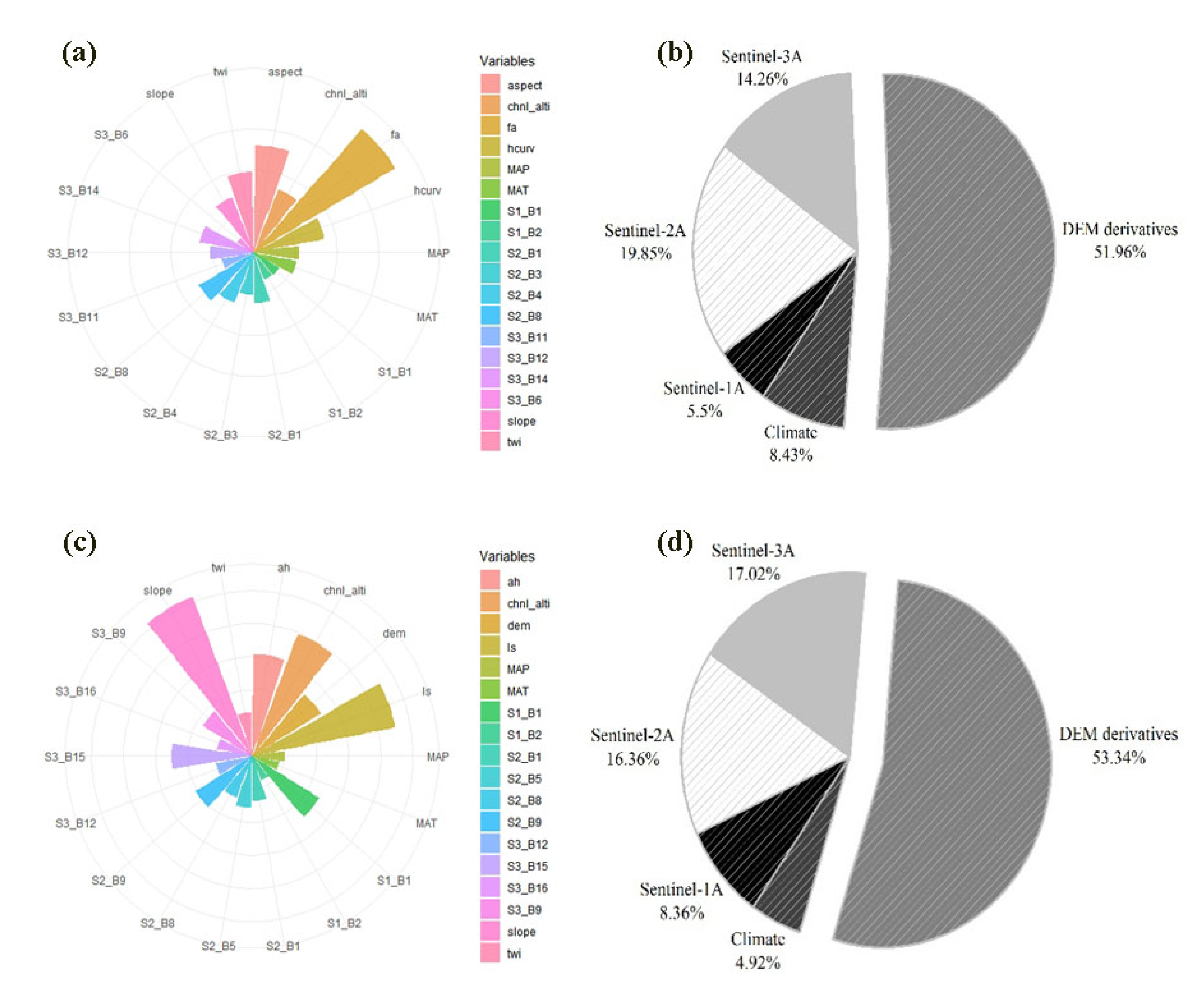
3.3. Importance Analysis of Environmental Variables

In this paper, all the selected link variables are correlated with SOC, and the importance ranking of the impact on SOC is analyzed (Figure 2). In combination with two models, RF and Cubist, the importance ranking of the two models is obtained. In the RF model (Figure 2a), the top three importances are Flow Accumulation, aspect, and twi, indicating that terrain is very important for prediction. The influence order of three different sensors is S-2 > S-3 > S-1. In terms of the proportion of importance (Figure 2b), DEM derivatives account for 54.96% of all levels of importance, followed by Sentinel-2A (19.85%), Sentinel-3A (14.26%), Sentinel-1A and climate (5.5% and 8.43%). In the Cubist model (Figure 2c,d), DEM derivatives accounted for 53.34%, but the proportion of Sentinel-3A was 17.02%, Sentinel-2A was 16.36%, Sentinel-1A and climate accounted for 8.36% and 4.92%, respectively. The most important DEM derivatives data were SLOP, LS and chnl _ alti. In the two models, DEM derivatives account for a large proportion of prediction, and the difference is that the proportion of Cubist is greater than that of RF. Among the sentinel data sources, Sentinel-2A has the greatest impact in the RF model, but Sentinel-3A accounts for the most important proportion in Cubist, and the climate proportion RF is greater than Cubist. It shows that the proportion of environmental variables is large under different models, and different data sources are selected by different models, indicating that the selection of models will also affect the prediction of SOC to a certain extent. It shows that the proportion of environmental variables is large under different models, and different data sources are selected by different models, indicating that the selection of models will also affect the prediction of SOC to a certain extent.

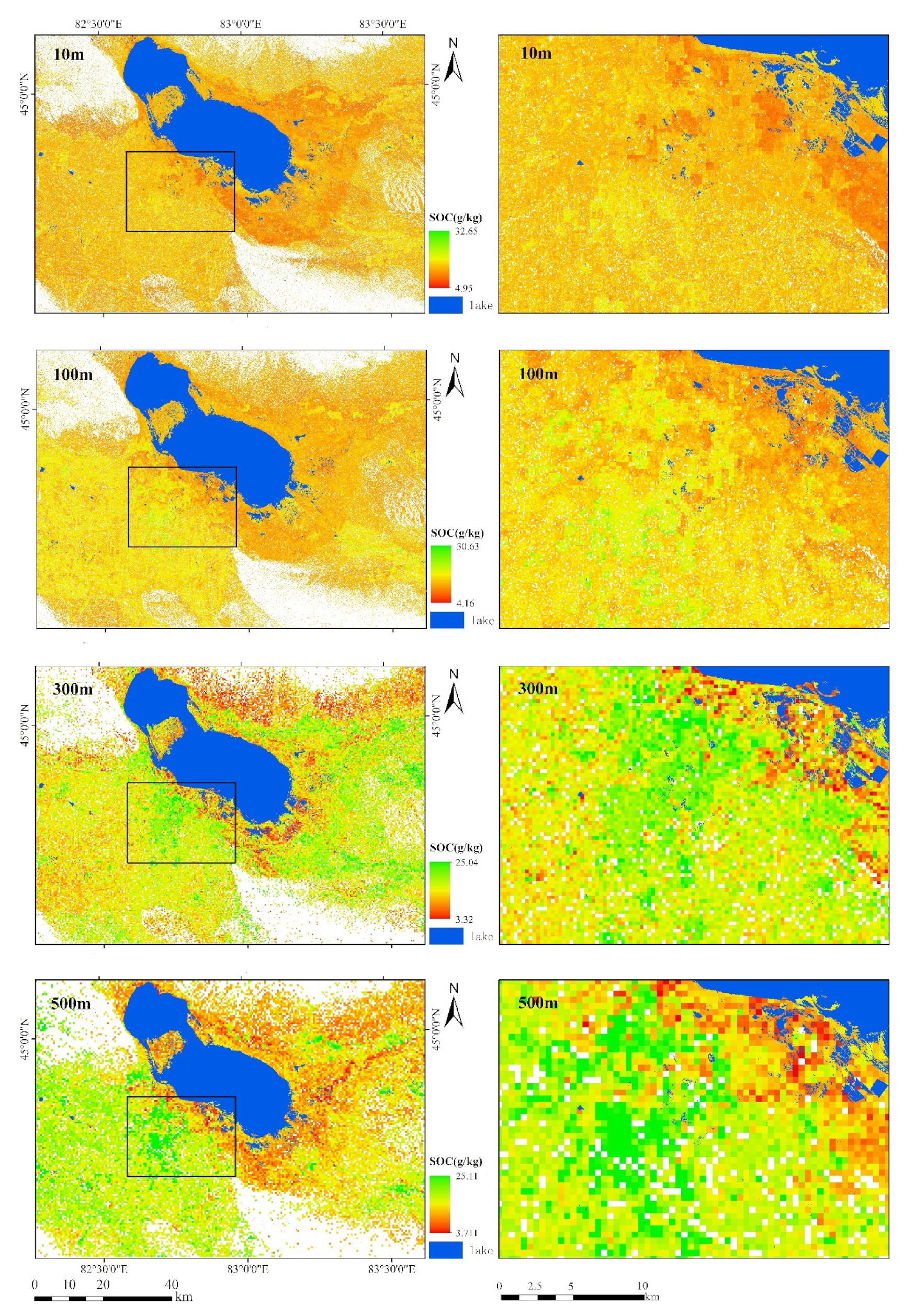
3.4. Spatial Prediction Results of SOC

The RF model has the highest prediction accuracy, and Figure 3 shows the SOC prediction map of model 7 at different spatial resolutions, with the lake mask on the image, as a way to determine the image location situation. From the four resolutions, the SOC distribution condition in the image changes as the resolution increases. From the selected locations, the SOC generally tends to be low at 10 and 100 m resolutions, with the mean values of the two resolutions being closer to 14.967 and 14.295, respectively. The 100 m mean value of 12.485 is closer to the predicted mean value than the measured value. The standard deviation of 10 m and 100 m is 6.459 and 8.112. The mean value of 300 m is 12.944 with a standard deviation of 2.475. The mean value for 500 m is 13.758 with a standard deviation of 3.787. Resolution is increasing, the image information is gradually blurred, and the prediction effect keeps changing.

4. Discussion

4.1. Sentinel-1A/2A/3A for SOC Prediction

In this article, two kinds of machine learning methods, RF and Cubist models, have been chosen for prediction of SOC distribution, and the RF model effects are shown in Figure 3. The prediction accuracy is described from different spatial resolution transformations. The two chosen prediction models have been accurately and effectively applied in soil organic carbon, and the accuracy of SOC prediction mapping has been confirmed [87]. In terms of overall model precision, the overall accuracy of the RF model was superior to the Cubist model, which is consistent with the results presented by Pouladi [81] in predicting soil organic matter distribution, who mapped and compared soil organic matter predictions by five models (Cubist, Random Forest, Cubist-kriging, Random Forest-kriging, Kriging) and obtained the same result as the model selected for this paper. Akpa [82] predicted SOC variation of different soil layers and the prediction showed that the RF model was slightly preferred to the Cubist model, and the classification of SOC at different resolutions has also been studied from the last few years [48]. However, SAR data were not analyzed with two different resolutions of spectral data. On this basis, SAR data are combined with optical data to serve as a data base for soil organic carbon prediction, and the predictive power of different types of data for digital mapping of soil organic carbon is explored.

In the prediction of soil organic carbon using Sentinel data, firstly, Sentinel-1A (SAR data) has the advantage in predicting soil and is better for most soil attribute data [88]. The use of Sentinel-1A as a covariate for soil organic carbon is less studied, but it cannot be denied that high-accuracy SAR data are a promising data source and effective in avoiding the effect of light sources on soil properties for remote sensing prediction of SOC [45]. Multispectral remote sensing data are no longer limited to for land use classification and are used to improve soil mapping accuracy while continuously improving remote sensing monitoring accuracy. Sentinel-2A data are well established in mapping and are used to improve mapping accuracy through different spectral resolutions and better signal-to-noise ratio in SWIR bands. The advantage of S-2 is that it has a clear advantage in quantitative mapping studies of SOC at different spatial scales, and that good matching between the two can be achieved [89]. The Sentinel-3A OLCI image contains bare soil spectrums band for the surface bare soil monitoring capability, and although the spatial resolution is lower, the short revisit period and large land coverage can provide more comprehensive data for predicting SOC [90]. Combining Sentinel-2A and Sentinel-3A spectral data can make up for the deficiencies of both in many aspects, and can enhance the graphical prediction to a collection of spectral resolution from small to medium to large scale, thus enriching the remote sensing monitoring of soil data by spectral data [48].

In the prediction of different data, the accuracy obtained by different models is shown in Table 5. The prediction accuracy of SAR data are better and superior to that of spectral data, and the complementary prediction effects of the two data sources in the spectral data model at different spatial resolutions can make the prediction results achieve their respective effects at different resolutions. In the study of kim [91], the effect of remote sensing modeling by different scales of spatial resolution data are more consistent with this study. In combining spectral data with DEM derivatives, the combination of radar data with environmental variables is better than that of spectral data, and the two data reflect their better prediction accuracy at different resolutions. In this paper, the data are divided into four scales to analyze the data variation in the case of different scale data. The multi-scale analysis can better reflect the direct influence of the selected data sources on the prediction results [48], and thus infer the optimal variables for SOC prediction analysis at different regional scales.

4.2. Analysis of Environmental Variables

The importance of DEM derivatives on SOC is highlighted in the importance plot (Figure 2). The various topographic attributes have some obvious influence on SOC [92], in agreement with the conclusions obtained in this paper, in terms of the different degrees of influence; SOC was strongly dependent on the topography and showed a certain distribution [93]. Surface soils are influenced by surface materials such as vegetation cover and deposition, water distribution and biological migration, and these characteristics all have an impact on the surface SOC of the soil [93]. Among the topographic factors, elevation, slope, and aspect were high in the order of importance, which is consistent with the conclusions obtained in this paper. Topography and slope play an important predictive role in DEM derivatives, and topography influences the variation of land surface biomass and thus the variation of SOC storage [94]. S.A.Bangroo [95] proposed in his study that topography have a direct influence on the distribution and spatial variation of SOC. Arun Mondal [96] concluded in a study that the change in SOC concentration decreases with increasing slope. Similarly, topographic indices such as TWI control the distribution of SOC in certain terrain, and TWI acts as an effective topographic factor to influence soil texture changes in terms of soil erosion and migration along with runoff calculations [97,98]. In this study, some DEM derivatives are also proposed to influence SOC prediction, such as fa, hcurv, chnl_alti, ls, ah; these indices also have some contribution to SOC prediction, Channel network will cause vegetation reduction to have some effect on surface cover change and thus affect soil change [99]. Adhikari, K [100] studied chnl_alti with wetness index, elevation, slope gradient, slope-length factor, as important topographic factors influencing the distribution of SOC in Denmark. Longitudinal Curvature [101] provides a good interpretation of the soil profile and geological structure and correlates surface material erosion with spatial distribution. Longitudinal curvature and analytical hill shading proved to be the most important environmental variables among the many DEM derivatives [102]. The prediction of SOC can provide effective environmental variables and can improve the prediction accuracy [103].

4.3. Comparison of Spatial Prediction Models

In this study, the digital soil mapping technique was used to obtain a soil organic carbon map for the Ebinur lake basin in the arid zone. For this study area, soil organic carbon mapping has not been studied, but the study of soil carbon storage and distribution characteristics will appear in previous studies [104]. For the spatial distribution of soil organic carbon (SOC), the main manifestation is the higher soil organic carbon content in the oasis region, a phenomenon that does not exclude the influence of human activities on SOC [105], while vegetation growth and withering processes and animal activities also contribute to this phenomenon [106]. The SOC content was lower in relatively wet and relatively dry environments, around water bodies and in desert areas, which is consistent with the results of [107]. SOC content varies with altitude, the higher the altitude the lower the SOC content, indicating a trend of SOC transport to lower altitudes [108,109]. Changes in temperature and precipitation due to altitude also have a significant effect on the distribution of SOC [16] and urbanization within oasis regions leads to higher temperature production [110], which in turn predicts that the areas with higher SOC in the figure are several major urban areas, and that SOC content decreases in areas with higher temperatures [111]. In contrast, the areas with more precipitation in the region are mostly higher-altitude mountainous areas, making the surface parent layer unstable can reduce the SOC distribution by being too dispersed [14]. The study area is located in an arid zone, where SOC distribution projections play an integral role in carbon stock estimation under the influence of climate change, human activities and topography [112,113,114].

5. Conclusions

In this study, the distribution of soil organic carbon in the arid zone was studied and analyzed by three data sources (S-1, S-2, and S-3) from two sensors (radar and optical) at four spatial resolutions (10, 100, 300, and 500 m) after two machine learning algorithms (RF, Cubist) to predict the SOC in the study area, and the following conclusions were obtained:

(1)

The simulation accuracies of the three data sources are ranked as Sentinel-1A (Model A) > Sentinel-2A (Model B) > Sentinel-3A (Model C). The prediction performance of the three data at different spatial resolutions is better for Sentinel-1A and Sentinel-2A at 10 m resolution and best for Sentinel-3A at 500 m.

(2)

Combining all environmental variables, the best model is model G. Model G is a combination of radar data, optical data and all environmental variables. In this model, the RF method has the best modeling effect at 10 m, R² = 0.406, MAE = 0.162, REMS = 5.947, LCCC = 0.266. In model E that combines SAR data with environmental variables, the prediction effect of 300 m is best to reach R² = 0.383. In model F that combines spectral data (S-2, S-3) with environmental variables, the 100 m prediction effect is best to reach R² = 0.397.

(3)

From the overall perspective, the accuracy of the RF model is better than that of Cubist among the two machine learning models, and the RF model can be used to predict SOC in arid areas in the future.

(4)

The spatial distribution of SOC shows that the SOC content is higher in oases, and lower in mountainous areas and areas around lake.

References

1. Lal, R. Soil carbon sequestration impacts on global climate change and food security. Science 2004, 304, 1623–1627. [Google Scholar] [CrossRef] [PubMed] [Green Version]
2. Lozano-García, B.; Francaviglia, R.; Renzi, G.; Doro, L.; Ledda, L.; Benítez, C.; González-Rosado, M.; Parras-Alcántara, L. Land use change effects on soil organic carbon store. An opportunity to soils regeneration in Mediterranean areas: Implications in the 4p1000 notion. Ecol. Indic. 2020, 119, 106831. [Google Scholar] [CrossRef]
3. Chen, L.-F.; He, Z.-B.; Du, J.; Yang, J.-J.; Zhu, X. Patterns and environmental controls of soil organic carbon and total nitrogen in alpine ecosystems of northwestern China. CATENA 2016, 137, 37–43. [Google Scholar] [CrossRef]
4. Dasandi, N.; Graham, H.; Lampard, P.; Jankin Mikhaylov, S. Engagement with health in national climate change commitments under the Paris Agreement: A global mixed-methods analysis of the nationally determined contributions. Lancet Planet. Health 2021, 5, e93–e101. [Google Scholar] [CrossRef]
5. Silatsa, F.B.T.; Yemefack, M.; Tabi, F.O.; Heuvelink, G.B.M.; Leenaars, J.G.B. Assessing countrywide soil organic carbon stock using hybrid machine learning modelling and legacy soil data in Cameroon. Geoderma 2020, 367, 114260. [Google Scholar] [CrossRef]
6. Batjes, N.H. Effects of mapped variation in soil conditions on estimates of soil carbon and nitrogen stocks for South America. Geoderma 2000, 97, 135–144. [Google Scholar] [CrossRef]
7. Yang, Y.; Mohammat, A.; Feng, J.; Zhou, R.; Fand, J. Storage, patterns and environmental Controls of soil organic Carbon in China. Biogeochemistry 2007, 84, 121–141. [Google Scholar] [CrossRef]
8. Yang, R.-M.; Zhang, G.-L.; Liu, F.; Lu, Y.-Y.; Yang, F.; Yang, F.; Yang, M.; Zhao, Y.-G.; Li, D.-C. Comparison of boosted regression tree and random forest models for mapping topsoil organic carbon concentration in an alpine ecosystem. Ecol. Indic. 2016, 60, 870–878. [Google Scholar] [CrossRef]
9. Mcbratney, A.; Santos, M.L.M.; Minasny, B. On Digital Soil Mapping. Geoderma 2003, 117, 3–52. [Google Scholar] [CrossRef]
10. Cinelli, G.; Tondeur, F.; Dehandschutter, B. Mapping potassium and thorium concentrations in Belgian soils. J. Environ. Radioact. 2018, 184–185, 127–139. [Google Scholar] [CrossRef]
11. Jeong, G.; Oeverdieck, H.; Park, S.J.; Huwe, B.; Ließ, M. Spatial soil nutrients prediction using three supervised learning methods for assessment of land potentials in complex terrain. CATENA 2017, 154, 73–84. [Google Scholar] [CrossRef]
12. John, K.; Isong, I.A.; Kebonye, N.M.; Ayito, E.O.; Agyeman, P.C.; Afu, S.M. Using Machine Learning Algorithms to Estimate Soil Organic Carbon Variability with Environmental Variables and Soil Nutrient Indicators in an Alluvial Soil. Land 2020, 9, 487. [Google Scholar] [CrossRef]
13. Guo, Z.; Adhikari, K.; Chellasamy, M.; Greve, M.B.; Owens, P.R.; Greve, M.H. Selection of terrain attributes and its scale dependency on soil organic carbon prediction. Geoderma 2019, 340, 303–312. [Google Scholar] [CrossRef]
14. Doetterl, S.; Stevens, A.; Six, J.; Merckx, R.; van Oost, K.; Casanova Pinto, M.; Casanova-Katny, A.; MuñOz, C.; Boudin, M.; Zagal Venegas, E. Soil carbon storage controlled by interactions between geochemistry and climate. Nat. Geosci. 2015. [Google Scholar] [CrossRef]
15. Xiong, X.; Grunwald, S.; Myers, D.B.; Kim, J.; Harris, W.G.; Comerford, N.B. Holistic environmental soil-landscape modeling of soil organic carbon. Environ. Model. Softw. 2014, 57, 202–215. [Google Scholar] [CrossRef]
16. Wiesmeier, M.; Urbanski, L.; Hobley, E.; Lang, B.; von Lützow, M.; Marin-Spiotta, E.; van Wesemael, B.; Rabot, E.; Ließ, M.; Garcia-Franco, N.; et al. Soil organic carbon storage as a key function of soils—A review of drivers and indicators at various scales. Geoderma 2019, 333, 149–162. [Google Scholar] [CrossRef]
17. Yang, R.M.; Zhang, G.L.; Yang, F.; Zhi, J.J.; Yang, F.; Liu, F.; Zhao, Y.G.; Li, D.C. Precise estimation of soil organic carbon stocks in the northeast Tibetan Plateau. Sci. Rep. 2015, 6, 21842. [Google Scholar] [CrossRef] [PubMed] [Green Version]
18. Arunrat, N.; Pumijumnong, N.; Hatano, R. Predicting local-scale impact of climate change on rice yield and soil organic carbon sequestration: A case study in Roi Et Province, Northeast Thailand. Agric. Syst. 2018, 164, 58–70. [Google Scholar] [CrossRef]
19. Jia, B.; Zhang, Z.; Ci, L.; Ren, Y.; Pan, B.; Zhang, Z. Oasis land-use dynamics and its influence on the oasis environment in Xinjiang, China. J. Arid Environ. 2004, 56, 11–26. [Google Scholar] [CrossRef]
20. Zhu, B.; Yu, J.; Qin, X.; Rioual, P.; Xiong, H. Climatic and geological factors contributing to the natural water chemistry in an arid environment from watersheds in northern Xinjiang, China. Geomorphology 2012, 153–154, 102–114. [Google Scholar] [CrossRef]
21. Yang, Z.; Gao, X.; Lei, J. Fuzzy comprehensive risk evaluation of aeolian disasters in Xinjiang, Northwest China. Aeolian Res. 2021, 48, 100647. [Google Scholar] [CrossRef]
22. Moore, I.D.; Gessler, P.E.; Nielsen, G.A.E.; Peterson, G.A. Soil Attribute Prediction Using Terrain Analysis. Soil Sci. Soc. Am. J. 1993, 57, 443–452. [Google Scholar] [CrossRef]
23. Odeh, I.O.A.; McBratney, A.B.; Chittleborough, D.J. Further results on prediction of soil properties from terrain attributes: Heterotopic cokriging and regression-kriging. Geoderma 1995, 67, 215–226. [Google Scholar] [CrossRef]
24. Stockmann, U.; Malone, B.P.; McBratney, A.B.; Minasny, B. Landscape-scale exploratory radiometric mapping using proximal soil sensing. Geoderma 2015, 239–240, 115–129. [Google Scholar] [CrossRef]
25. Malone, B.P.; Jha, S.K.; Minasny, B.; McBratney, A.B. Comparing regression-based digital soil mapping and multiple-point geostatistics for the spatial extrapolation of soil data. Geoderma 2016, 262, 243–253. [Google Scholar] [CrossRef]
26. Hartemink, A.E.; Krasilnikov, P.; Bockheim, J.G. Soil maps of the world. Geoderma 2013, 207–208, 256–267. [Google Scholar] [CrossRef]
27. Iticha, B.; Takele, C. Digital soil mapping for site-specific management of soils. Geoderma 2019, 351, 85–91. [Google Scholar] [CrossRef]
28. Were, K.; Bui, D.T.; Dick, Ø.B.; Singh, B.R. A comparative assessment of support vector regression, artificial neural networks, and random forests for predicting and mapping soil organic carbon stocks across an Afromontane landscape. Ecol. Indic. 2015, 52, 394–403. [Google Scholar] [CrossRef]
29. Tajik, S.; Ayoubi, S.; Zeraatpisheh, M. Digital mapping of soil organic carbon using ensemble learning model in Mollisols of Hyrcanian forests, northern Iran. Geoderma Reg. 2020, 20, e00256. [Google Scholar] [CrossRef]
30. Castaldi, F.; Hueni, A.; Chabrillat, S.; Ward, K.; Buttafuoco, G.; Bomans, B.; Vreys, K.; Brell, M.; van Wesemael, B. Evaluating the capability of the Sentinel 2 data for soil organic carbon prediction in croplands. ISPRS J. Photogramm. Remote Sens. 2019, 147, 267–282. [Google Scholar] [CrossRef]
31. Sayão, V.M.; Demattê, J.A.M. Soil texture and organic carbon mapping using surface temperature and reflectance spectra in Southeast Brazil. Geoderma Reg. 2018, 14, e00174. [Google Scholar] [CrossRef]
32. Gholizadeh, A.; Žižala, D.; Saberioon, M.; Borůvka, L. Soil organic carbon and texture retrieving and mapping using proximal, airborne and Sentinel-2 spectral imaging. Remote Sens. Environ. 2018, 218, 89–103. [Google Scholar] [CrossRef]
33. Berger, M.; Moreno, J.; Johannessen, J.A.; Levelt, P.F.; Hanssen, R.F. ESA’s sentinel missions in support of Earth system science. Remote Sens. Environ. 2012, 120, 84–90. [Google Scholar] [CrossRef]
34. Dkhala, B.; Mezned, N.; Gomez, C.; Abdeljaouad, S. Hyperspectral field spectroscopy and SENTINEL-2 Multispectral data for minerals with high pollution potential content estimation and mapping. Sci. Total Environ. 2020, 740, 140160. [Google Scholar] [CrossRef]
35. Gomez, C.; Adeline, K.; Bacha, S.; Driessen, B.; Gorretta, N.; Lagacherie, P.; Roger, J.M.; Briottet, X. Sensitivity of clay content prediction to spectral configuration of VNIR/SWIR imaging data, from multispectral to hyperspectral scenarios. Remote Sens. Environ. 2018, 204, 18–30. [Google Scholar] [CrossRef]
36. Belluco, E.; Camuffo, M.; Ferrari, S.; Modenese, L.; Silvestri, S.; Marani, A.; Marani, M. Mapping salt-marsh vegetation by multispectral and hyperspectral remote sensing. Remote Sens. Environ. 2006, 105, 54–67. [Google Scholar] [CrossRef]
37. Wielemaker, W.G.; de Bruin, S.; Epema, G.F.; Veldkamp, A. Significance and application of the multi-hierarchical landsystem in soil mapping. CATENA 2001, 43, 15–34. [Google Scholar] [CrossRef]
38. Logsdon, S.D.; Perfect, E.; Tarquis, A.M. Multiscale Soil Investigations: Physical Concepts and Mathematical Techniques. Vadose Zone J. 2008, 7, 453–455. [Google Scholar] [CrossRef] [Green Version]
39. Viaa, R.; Magillo, P.; Puppo, E. Multi-Scale Geographic Maps; Springer: Berlin/Heidelberg, Germany, 2005. [Google Scholar]
40. Dumont, M.; Touya, G.; Duchêne, C. Designing multi-scale maps: Lessons learned from existing practices. Int. J. Cartogr. 2020, 6, 121–151. [Google Scholar] [CrossRef]
41. Pahlavan-Rad, M.R.; Dahmardeh, K.; Brungard, C. Predicting soil organic carbon concentrations in a low relief landscape, eastern Iran. Geoderma Reg. 2018, 15, e00195. [Google Scholar] [CrossRef]
42. Huang, X.; Senthilkumar, S.; Kravchenko, A.; Thelen, K.; Qi, J. Total carbon mapping in glacial till soils using near-infrared spectroscopy, Landsat imagery and topographical information. Geoderma 2007, 141, 34–42. [Google Scholar] [CrossRef]
43. Dou, X.; Wang, X.; Liu, H.; Zhang, X.; Meng, L.; Pan, Y.; Yu, Z.; Cui, Y. Prediction of soil organic matter using multi-temporal satellite images in the Songnen Plain, China. Geoderma 2019, 356, 113896. [Google Scholar] [CrossRef]
44. Yang, R.-M.; Guo, W.-W. Modelling of soil organic carbon and bulk density in invaded coastal wetlands using Sentinel-1 imagery. Int. J. Appl. Earth Obs. Geoinf. 2019, 82, 101906. [Google Scholar] [CrossRef]
45. Liu, B.; D’Sa, E.J.; Joshi, I. Multi-decadal trends and influences on dissolved organic carbon distribution in the Barataria Basin, Louisiana from in-situ and Landsat/MODIS observations. Remote Sens. Environ. 2019, 228, 183–202. [Google Scholar] [CrossRef]
46. Lin, C.; Zhu, A.X.; Wang, Z.; Wang, X.; Ma, R. The refined spatiotemporal representation of soil organic matter based on remote images fusion of Sentinel-2 and Sentinel-3. Int. J. Appl. Earth Obs. Geoinf. 2020, 89, 102094. [Google Scholar] [CrossRef]
47. Zhou, T.; Geng, Y.; Chen, J.; Pan, J.; Haase, D.; Lausch, A. High-resolution digital mapping of soil organic carbon and soil total nitrogen using DEM derivatives, Sentinel-1 and Sentinel-2 data based on machine learning algorithms. Sci. Total Environ. 2020, 729, 138244. [Google Scholar] [CrossRef] [PubMed]
48. Zhou, T.; Geng, Y.; Ji, C.; Xu, X.; Wang, H.; Pan, J.; Bumberger, J.; Haase, D.; Lausch, A. Prediction of soil organic carbon and the C:N ratio on a national scale using machine learning and satellite data: A comparison between Sentinel-2, Sentinel-3 and Landsat-8 images. Sci. Total Environ. 2021, 755, 142661. [Google Scholar] [CrossRef]
49. Ge, Y.; Abuduwaili, J.; Ma, L.; Wu, N.; Liu, D. Potential transport pathways of dust emanating from the playa of Ebinur Lake, Xinjiang, in arid northwest China. Atmos. Res. 2016, 178–179, 196–206. [Google Scholar] [CrossRef]
50. Hao, S.; Li, F.; Li, Y.; Gu, C.; Zhang, Q.; Qiao, Y.; Jiao, L.; Zhu, N. Stable isotope evidence for identifying the recharge mechanisms of precipitation, surface water, and groundwater in the Ebinur Lake basin. Sci. Total Environ. 2019, 657, 1041–1050. [Google Scholar] [CrossRef]
51. Yushanjiang, A.; Zhang, F.; Yu, H.; Kung, H. Quantifying the spatial correlations between landscape pattern and ecosystem service value: A case study in Ebinur Lake Basin, Xinjiang, China. Ecol. Eng. 2018, 113, 94–104. [Google Scholar] [CrossRef]
52. Wang, J.; Ding, J.; Yu, D.; Ma, X.; Zhang, Z.; Ge, X.; Teng, D.; Li, X.; Liang, J.; Lizaga, I.; et al. Capability of Sentinel-2 MSI data for monitoring and mapping of soil salinity in dry and wet seasons in the Ebinur Lake region, Xinjiang, China. Geoderma 2019, 353, 172–187. [Google Scholar] [CrossRef]
53. Nawar, S.; Mouazen, A.M. On-line vis-NIR spectroscopy prediction of soil organic carbon using machine learning. Soil Tillage Res. 2019, 190, 120–127. [Google Scholar] [CrossRef]
54. Nelson, D. A rapid and accurate method for estimating organic carbon in soil. Proc. Indiana Acad. Sci. 1975, 84, 456–462. [Google Scholar]
55. Conrad, O.; Bechtel, B.; Bock, M.; Dietrich, H.; Fischer, E.; Gerlitz, L.; Wehberg, J.; Wichmann, V.; Böhner, J. System for Automated Geoscientific Analyses (SAGA) v. 2.1.4. Geosci. Model Dev. 2015, 8, 1991–2007. [Google Scholar] [CrossRef] [Green Version]
56. Quinn, P.; Beven, K.; Chevallier, P.; Planchon, O. The prediction of hillslope flow paths for distributed hydrological modelling using digital terrain models. Hydrol. Process. 2010, 5, 59–79. [Google Scholar] [CrossRef]
57. Wood, J. Chapter 14 Geomorphometry in LandSerf. In Developments in Soil Science; Hengl, T., Reuter, H.I., Eds.; Elsevier: Amsterdam, The Netherlands, 2009; pp. 333–349. ISBN 0166-2481. [Google Scholar]
58. Iwahashi, J.; Pike, R.J. Automated classifications of topography from DEMs by an unsupervised nested-means algorithm and a three-part geometric signature. Geomorphology 2007, 86, 409–440. [Google Scholar] [CrossRef]
59. Cheng, Z.Q.; Zhan, L.J. Parallelizing flow-accumulation calculations on graphics processing units-From iterative DEM preprocessing algorithm to recursive multiple-flow-direction algorithm. Comput. Geosci. 2012, 43, 7–16. [Google Scholar]
60. Gallant, J.C.; Dowling, T.I. A multiresolution index of valley bottom flatness for mapping depositional areas. Water Resour. Res. 2003, 39, 291–297. [Google Scholar] [CrossRef]
61. Bock, M.; Köthe, R. Predicting the Depth of Hydromorphic Soil Haracteristics Influenced by Ground Water. SAGA—Seconds Out 2008, 19, 13–22. [Google Scholar]
62. Rodriguez, F. The Black Top Hat function applied to a DEM: A tool to estimate recent incision in a mountainous watershed (Estibère Watershed, Central Pyrenees). Geophys. Res. Lett. 2002, 29. [Google Scholar] [CrossRef] [Green Version]
63. Dawen, Y.; Srikantha, H.; Katumi, M. A hillslope-based hydrological model using catchment area and width functions. Hydrol. Sci. J. 2002, 47, 49–65. [Google Scholar]
64. Böhner, T.S.J. Spatial prediction of soil attributes using terrain analysis and climate regionalisation. SAGA–Analyses and Modelling Applications. Göttinger Geogr. Abh. 2006, 115, 13–28. [Google Scholar]
65. Hong, S.H.; Wdowinski, S. Evaluation of the quad-polarimetric Radarsat-2 observations for the wetland InSAR application. Can. J. Remote Sens. 2012, 37, 484–492. [Google Scholar] [CrossRef] [Green Version]
66. Wang, C.; Pan, Y.; Chen, J.; Ouyang, Y.; Rao, J.; Jiang, Q. Indicator element selection and geochemical anomaly mapping using recursive feature elimination and random forest methods in the Jingdezhen region of Jiangxi Province, South China. Appl. Geochem. 2020, 122, 104760. [Google Scholar] [CrossRef]
67. Zhou, T.; Zhao, M.; Sun, C.; Pan, J. Exploring the impact of seasonality on urban land-cover mapping using multi-season sentinel-1A and GF-1 WFV images in a subtropical monsoon-climate region. ISPRS Int. J. Geo-Inf. 2018, 7, 3. [Google Scholar]
68. Louis, J.; Debaecker, V.; Pflug, B.; Main-Knorn, M.; Bieniarz, J.; Müller-Wilm, U.; Cadau, E.G.; Gascon, F. SENTINEL-2 SEN2COR: L2A Processor for Users. In Proceedings of the ESA Living Planet Symposium, Prague, Czech Republic, 9–13 May 2016. [Google Scholar]
69. Yue, T.X.; Zhao, N.; Ramsey, R.D.; Wang, C.L.; Fan, Z.M.; Chen, C.F.; Lu, Y.M.; Li, B.L. Climate change trend in China, with improved accuracy. Clim. Chang. 2013, 120, 137–151. [Google Scholar] [CrossRef]
70. Jeung, M.; Baek, S.; Beom, J.; Cho, K.H.; Her, Y.; Yoon, K. Evaluation of random forest and regression tree methods for estimation of mass first flush ratio in urban catchments. J. Hydrol. 2019, 575, 1099–1110. [Google Scholar] [CrossRef]
71. Zhou, X.; Wang, P.; Tansey, K.; Zhang, S.; Li, H.; Tian, H. Reconstruction of time series leaf area index for improving wheat yield estimates at field scales by fusion of Sentinel-2, -3 and MODIS imagery. Comput. Electron. Agric. 2020, 177, 105692. [Google Scholar] [CrossRef]
72. Pal, M.; Giles, M.F. Feature Selection for Classification of Hyperspectral Data by SVM. IEEE Trans. Geosci. Remote Sens. 2010, 48, 2297–2307. [Google Scholar] [CrossRef] [Green Version]
73. Khosravi, I.; Alavipanah, S.K. A random forest-based framework for crop mapping using temporal, spectral, textural and polarimetric observations. Int. J. Remote Sens. 2019, 40, 7221–7251. [Google Scholar] [CrossRef]
74. Wang, B.; Waters, C.; Orgill, S.; Cowie, A.; Clark, A.; de Li, L.; Simpson, M.; McGowen, I.; Sides, T. Estimating soil organic carbon stocks using different modelling techniques in the semi-arid rangelands of eastern Australia. Ecol. Indic. 2018, 88, 425–438. [Google Scholar] [CrossRef]
75. Appelhans, T.; Mwangomo, E.; Hardy, D.R.; Hemp, A.; Nauss, T. Evaluating machine learning approaches for the interpolation of monthly air temperature at Mt. Kilimanjaro, Tanzania. Spat. Stat. 2015, 14, 91–113. [Google Scholar] [CrossRef] [Green Version]
76. Ma, Z.; Shi, Z.; Zhou, Y.; Xu, J.; Yu, W.; Yang, Y. A spatial data mining algorithm for downscaling TMPA 3B43 V7 data over the Qinghai–Tibet Plateau with the effects of systematic anomalies removed. Remote Sens. Environ. 2017, 200, 378–395. [Google Scholar] [CrossRef]
77. Bui, E.; Henderson, B.; Viergever, K. Using knowledge discovery with data mining from the Australian Soil Resource Information System database to inform soil carbon mapping in Australia. Glob. Biogeochem. Cycles 2009, 23. [Google Scholar] [CrossRef]
78. Walton, J.T. Subpixel urban land cover estimation: Comparing cubist, random forests, and support vector regression. Photogramm. Eng. Remote Sens. 2008, 74, 1213–1222. [Google Scholar] [CrossRef] [Green Version]
79. Houborg, R.; Mccabe, M.F. A hybrid training approach for leaf area index estimation via Cubist and random forests machine-learning. Isprs J. Photogramm. Remote Sens. Environ. 2017, 135, 173–188. [Google Scholar] [CrossRef]
80. Henderson, B.L.; Bui, E.N.; Moran, C.J.; Simon, D.A.P. Australia-wide predictions of soil properties using decision trees. Geoderma 2005, 124, 383–398. [Google Scholar] [CrossRef]
81. Pouladi, N.; Møller, A.B.; Tabatabai, S.; Greve, M.H. Mapping soil organic matter contents at field level with Cubist, Random Forest and kriging. Geoderma 2019, 342, 85–92. [Google Scholar] [CrossRef]
82. Akpa, S.I.C.; Odeh, I.O.A.; Bishop, T.F.A.; Hartemink, A.E.; Amapu, I.Y. Total soil organic carbon and carbon sequestration potential in Nigeria. Geoderma 2016, 271, 202–215. [Google Scholar] [CrossRef]
83. Miller, B.A.; Koszinski, S.; Wehrhan, M.; Sommer, M. Comparison of spatial association approaches for landscape mapping of soil organic carbon stocks. Soil 2015, 1, 217–233. [Google Scholar] [CrossRef] [Green Version]
84. Amirian-Chakan, A.; Minasny, B.; Taghizadeh-Mehrjardi, R.; Akbarifazli, R.; Darvishpasand, Z.; Khordehbin, S. Some practical aspects of predicting texture data in digital soil mapping. Soil Tillage Res. 2019, 194, 104289. [Google Scholar] [CrossRef]
85. Fabio, C.; Sabine, C.; Arwyn, J.; Kristin, V.; Bart, B.; van Bas, W. Soil Organic Carbon Estimation in Croplands by Hyperspectral Remote APEX Data Using the LUCAS Topsoil Database. Remote Sens. 2018, 10, 153. [Google Scholar]
86. Kuei, I.; Lin, L. A concordance correlation coefficient to evaluate reproducibility. Biometrics 1989, 45, 255–268. [Google Scholar]
87. Wiesmeier, M.; Barthold, F.; Blank, B.; Ingrid, K.-K. Digital mapping of soil organic matter stocks using Random Forest modeling in a semi-arid steppe ecosystem. Plant Soil 2011, 340, 7–24. [Google Scholar] [CrossRef]
88. Yang, R.-M.; Guo, W.-W.; Zheng, J.-B. Soil prediction for coastal wetlands following Spartina alterniflora invasion using Sentinel-1 imagery and structural equation modeling. CATENA 2019, 173, 465–470. [Google Scholar] [CrossRef]
89. Stevens, A.; Udelhoven, T.; Denis, A.; Tychon, B.; Lioy, R.; Hoffmann, L.; van Wesemael, B. Measuring soil organic carbon in croplands at regional scale using airborne imaging spectroscopy. Geoderma 2010, 158, 32–45. [Google Scholar] [CrossRef]
90. Li, W.; Niu, Z.; Shang, R.; Qin, Y.; Wang, L.; Chen, H. High-resolution mapping of forest canopy height using machine learning by coupling ICESat-2 LiDAR with Sentinel-1, Sentinel-2 and Landsat-8 data. Int. J. Appl. Earth Obs. Geoinf. 2020, 92, 102163. [Google Scholar] [CrossRef]
91. Kim, J.; Grunwald, S.; Rivero, R.G.; Rick, R. Multi-scale Modeling of Soil Series Using Remote Sensing in a Wetland Ecosystem. Soil Sci. Soc. Am. J. 2012, 76, 2327. [Google Scholar] [CrossRef]
92. Yu, H.; Zha, T.; Zhang, X.; Nie, L.; Ma, L.; Pan, Y. Spatial distribution of soil organic carbon may be predominantly regulated by topography in a small revegetated watershed. CATENA 2020, 188, 104459. [Google Scholar] [CrossRef]
93. Yoo, K.; Amundson, R.; Heimsath, A.M.; Dietrich, W.E. Spatial patterns of soil organic carbon on hillslopes: Integrating geomorphic processes and the biological C cycle. Geoderma 2006, 130, 47–65. [Google Scholar] [CrossRef]
94. Zhang, X.; Liu, M.; Zhao, X.; Li, Y.; Zhao, W.; Li, A.; Chen, S.; Chen, S.; Han, X.; Huang, J. Topography and grazing effects on storage of soil organic carbon and nitrogen in the northern China grasslands. Ecol. Indic. 2018, 93, 45–53. [Google Scholar] [CrossRef]
95. Bangroo, S.A.; Najar, G.R.; Achin, E.; Truong, P.N. Application of predictor variables in spatial quantification of soil organic carbon and total nitrogen using regression kriging in the North Kashmir forest Himalayas. CATENA 2020, 193, 104632. [Google Scholar] [CrossRef]
96. Mondal, A.; Khare, D.; Kundu, S.; Mondal, S.; Mukherjee, S.; Mukhopadhyay, A. Spatial soil organic carbon (SOC) prediction by regression kriging using remote sensing data. Egypt. J. Remote Sens. Space Sci. 2017, 20, 61–70. [Google Scholar] [CrossRef] [Green Version]
97. Schwanghart, W.; Jarmer, T. Linking spatial patterns of soil organic carbon to topography—A case study from south-eastern Spain. Geomorphology 2011, 126, 252–263. [Google Scholar] [CrossRef]
98. Cantón, Y.; Solé-Benet, A.; Domingo, F. Temporal and spatial patterns of soil moisture in semiarid badlands of SE Spain. J. Hydrol. 2004, 285, 199–214. [Google Scholar] [CrossRef]
99. Liu, Z.; Fagherazzi, S.; She, X.; Ma, X.; Xie, C.; Cui, B. Efficient tidal channel networks alleviate the drought-induced die-off of salt marshes: Implications for coastal restoration and management. Sci. Total Environ. 2020, 749, 141493. [Google Scholar] [CrossRef]
100. Kabindra, A.; Hartemink, A.E.; Budiman, M.; Rania, B.K.; Greve, M.B.; Greve, M.H.; Hui, D. Digital Mapping of Soil Organic Carbon Contents and Stocks in Denmark. PLoS ONE 2014, 9, e105519. [Google Scholar]
101. Farrokhzad, F.; Barari, A.; Choobbasti, A.J.; Ibsen, L.B. Neural network-based model for landslide susceptibility and soil longitudinal profile analyses: Two case studies. J. Afr. Earth Sci. 2011, 61, 349–357. [Google Scholar] [CrossRef]
102. Mashalaba, L.; Galleguillos, M.; Seguel, O.; Poblete-Olivares, J. Predicting spatial variability of selected soil properties using digital soil mapping in a rainfed vineyard of central Chile. Geoderma Reg. 2020, 22, e00289. [Google Scholar] [CrossRef]
103. Liu, S.; An, N.; Yang, J.; Dong, S.; Wang, C.; Yin, Y. Prediction of soil organic matter variability associated with different land use types in mountainous landscape in southwestern Yunnan province, China. CATENA 2015, 133, 137–144. [Google Scholar] [CrossRef]
104. Xu, H.; Zeng, C.; Wang, W.; Zhai, J. Study on Vertical Distribution and the Influencing Factors of Soil Organic Carbon in Ebinur Lake Wetland. J. Fujian Norm. Univ. 2010, 26, 92–97. [Google Scholar]
105. Qi, Q.; Zhang, D.; Zhang, M.; Tong, S.; Wang, W.; An, Y. Spatial distribution of soil organic carbon and total nitrogen in disturbed Carex tussock wetland. Ecol. Indic. 2021, 120, 106930. [Google Scholar] [CrossRef]
106. Chen, W.; Ge, Z.-M.; Fei, B.-L.; Chao, Z.; Liu, Q.-X.; Zhang, L.-Q. Soil carbon and nitrogen storage in recently restored and mature native Scirpus marshes in the Yangtze Estuary, China: Implications for restoration. Ecol. Eng. 2017, 104, 150–157. [Google Scholar] [CrossRef]
107. Hobley, E.U.; Baldock, J.; Wilson, B. Environmental and human influences on organic carbon fractions down the soil profile. Agric. Ecosyst. Environ. 2016, 223, 152–166. [Google Scholar] [CrossRef] [Green Version]
108. Knoepp, J.D.; See, C.R.; Vose, J.M.; Miniat, C.F.; Clark, J.S. Total C and N Pools and Fluxes Vary with Time, Soil Temperature, and Moisture Along an Elevation, Precipitation, and Vegetation Gradient in Southern Appalachian Forests. Ecosystems 2018, 21, 1623–1638. [Google Scholar] [CrossRef]
109. Fu, X.; Shao, M.; Wei, X.; Horton, R. Soil organic carbon and total nitrogen as affected by vegetation types in Northern Loess Plateau of China. Geoderma 2010, 155, 31–35. [Google Scholar] [CrossRef]
110. Wiesmeier, M.; Barthold, F.; Spörlein, P.; Geuß, U.; Hangen, E.; Reischl, A.; Schilling, B.; Angst, G.; von Lützow, M.; Kögel-Knabner, I. Estimation of total organic carbon storage and its driving factors in soils of Bavaria (southeast Germany). Geoderma Reg. 2014, 1, 67–78. [Google Scholar] [CrossRef]
111. Koven, C.D.; Hugelius, G.; Lawrence, D.M.; Wieder, W.R. Higher climatological temperature sensitivity of soil carbon in cold than warm climates. Nat. Clim. Chang. 2017, 7, 817–822. [Google Scholar] [CrossRef] [Green Version]
112. Xu, E.; Zhang, H.; Xu, Y. Exploring land reclamation history: Soil organic carbon sequestration due to dramatic oasis agriculture expansion in arid region of Northwest China. Ecol. Indic. 2020, 108, 105746. [Google Scholar] [CrossRef]
113. Kopittke, P.M.; Dalal, R.C.; Finn, D.; Menzies, N.W. Global changes in soil stocks of carbon, nitrogen, phosphorus, and sulphur as influenced by long-term agricultural production. Glob. Chang. Biol. 2017, 23, 2509–2519. [Google Scholar] [CrossRef]
114. Wichern, F.; Luedeling, E.; Müller, T.; Joergensen, R.G.; Buerkert, A. Field measurements of the CO2 evolution rate under different crops during an irrigation cycle in a mountain oasis of Oman. Appl. Soil Ecol. 2004, 25, 85–91. [Google Scholar] [CrossRef]
Figure 1. Study area located in Xinjiang and (A) Sentinel-1 image, (B) Sentinel-2 image and (C) Sentinel-3 image.
Remotesensing 13 00769 g001
Figure 2. Importance assignment of environment variables ((a) is the importance ranking of the environmental variables of the RF model, (b) is the importance of the data of different environmental variables in the RF model, (c) is the importance ranking of the environmental variables of the Cubist model, and (d) is the importance of the data of different environmental variables in the Cubist model).
Remotesensing 13 00769 g002
Figure 3. RF-predicted SOC distribution of model G at resolutions (10, 100, 300, and 500 m).
Remotesensing 13 00769 g003