Abstract
With the ongoing trend towards deep learning in the remote sensing community, classical pixel based algorithms are often outperformed by convolution based image segmentation algorithms. This performance was mostly validated spatially, by splitting training and validation pixels for a given year. Though generalizing models temporally is potentially more difficult, it has been a recent trend to transfer models from one year to another, and therefore to validate temporally. The study argues that it is always important to check both, in order to generate models that are useful beyond the scope of the training data. It shows that convolutional neural networks have potential to generalize better than pixel based models, since they do not rely on phenological development alone, but can also consider object geometry and texture. The UNET classifier was able to achieve the highest F1 scores, averaging 0.61 in temporal validation samples, and 0.77 in spatial validation samples. The theoretical potential for overfitting geometry and just memorizing the shape of fields that are maize has been shown to be insignificant in practical applications. In conclusion, kernel based convolutions can offer a large contribution in making agricultural classification models more transferable, both to other regions and to other years.
1. Introduction
1.1. State of the Art
The remote sensing community in general, and the land use/land cover (LULC) classification community in particular, is currently in a stage where potential applications seem endless [1], high resolution satellite imagery at national levels is available for free [2], and sophisticated classification algorithms perform better with each new generation [3]. This is especially true for the field of agricultural crop classification, where many studies were published in the past 5 years, that implemented one of many different iterations of deep learnig algorithms. In these studies, the model input has been rather stable, mostly consisting of multispectral global sensors like Landsat [4], Synthetic Aparture Radar (SAR) satellites like Sentinel-1 [5] and very high resolution optical sensors like Gaofen [6] as well as combinations of optical and SAR sensors [7]. The SAR domain has seen some advances in data processing techniques, where the phase information of polarimetric radar imagery can be used to derive parameters of the scattering. Parameters like anisotropy/entropy [8] and double bounce/surface/volume scattering [9] can be used to classify LULC and even radar based vegetation indices can be derived [10]. While there were some advances in the processing of the input datasets, model algorithms have almost completely switched from traditional machine learning and classical neural network algorithms, over Convolutional Neural Networks (CNN) and autoencoders [11] towards advanced derivates of the CNN approach like UNET [12] or the Recurrent Neural Network (RNN) approach like Long Short Term Memory (LSTM) models [13].
Another visible trend in the past 5 years, is that an increasing number of papers start to assess temporal model generalization. In the beginning, for example in case studies in India [14], the Ukraine [15] and Brazil [16], validation data was split spatially. This means that pixels or fields from one single scene, or one single mosaick were taken out of the training dataset and split into two or three sets of training, validation and testing samples. Cai et al. [17] were successfully able to test the temporal transferability of a Neural Network based corn and soybean classifier. They used long term Landsat derived vegetation index time series, and were able to predict years that were not part of the training datasets with high accuracy. Momm, ElKadiri and Porter [18] also used Landsat NDVI time series to classifiy crop types in the United States, and systematically tested models based on 2005 data with data from the year 2000 and vice versa. Zhang et al. [6] went a different approach and did not rely on index based phenlogy curves. They used high resolution satellite imagery to delineate cropland and non-cropland in several chinese regions, while testing both spatial and temporal transferability of their CNN models. The temporal transferability was tested by applying models from 2016 to 2017, and the spatial transferability was tested on different regions. Ajadi et al. [19] classified soybean and corn crops in brasil based on a composite of optical and SAR imagery, and also tested spatial and temporal transferability of their models by testing a model trained in summer 2017–2018 with a dataset from summer 2018–2019 and from a different state.
Though there is a clear trend in these case studies, to value transferability considerations in model assessment, recent review papers focused on the topics of deep learning in remote sensing and crop classification [20,21,22] do not cover transferability considerations at all. Olofsson et al. [23] mention the importance of stratified randomization in the sampling process, but do not specificy the nature of these strata any further. Though generalization has been an important concept in remote sensing based classifaction for more than a decade [24], and strategies exist to asses it on a technical level (sampel splitting, crossvalidation), there is no clear definition or discussion about the way the validation and testing datasets need to be different from the training datasets, in order to say that a model generalizes well.
1.2. Objectives
The goal of this study is to add to this discussion by introducing a novel way to frame the model validation process. It will be described by a number of different scopes on a similarity spectrum where distance is implied, but not quantifiable. Its premise will be, that a high performance classification in the closest scope (within-scene) is achievable by many different simple and complex algorithms, but is not enough to evaluate a models usefulness. Good performance in scopes that are very far from the training scopes on the other hand are increasingly impossible, as summarized in the No Free Lunch Theorem [25,26]. The concept of temporal and spatial validation scopes will be used to compare the transferability and generalization of classical pixel based algorithms to contemporary convolution based approaches in the context of remote sensing analysis, using the example of binary maize classification. The quantification and localization of silage maize expansion has been shown to be a very important part of the environmental monitoring process in southwest Germany [27]. While pixel based statistical and machine learning algorithms are well suited to classify agricultural use based on optical remote sensing imagery [28], a reliable modeling approach that is able to classify across the entire region and for any given year is still not yet identified. In this study, we try to take advantage of the aforementioned progress in the field of deep learning and CNNs, while at the same time using multitemporal SAR composites as a way to consistently acquire data for the entire study region for 4 years from 2016 to 2019. While many studies were able to produce deep learning models with high performance and highlight their superiority over classifcal machine learning, a fully randomized design is going to improve the understanding of how well this translates to improved performance in out of training samples. The goals of this study in more detail:
- Input Data:In order to validate temporal transferability, there is a requirement for consistency between years. For this reason, Sentinel-1 scenes will be processed in a way to generate monthly average based timeseries to reflect crop phenology.
- Validation Scopes:Scopes will be defined as subsets of the entire dataset. Aside from the training scope, there will be scopes that test spatial and temporal transferability, as well as both combined. To check for potential overfitting of field shapes and memory effects, special within geometry scopes will be defined and tested for predictive inconsistencies.
- Model Training and Evaluation:Based on the defined scopes, 500 sets of samples are randomly drawn. Two representative pixel based and two representative convolution based classifiers are trained, and the model performances are measured for each scope independently. Finally, the sampled model performances are evaluated with parameter free U-tests, in order to infer which algorithms perform better in any given scope.
2. Materials and Methods
2.1. Study Area
The administrative district “Eifelkreis Bitburg-Prüm” (in the following referred to as ‘study area’, see Figure 1) has been shown to be a perfectly suitable region for crop classification studies before [28]. It is located in the center of Europe, but still shows very little segmentation by settlements, and offers a comparatively homogenous landscape dominated by agriculture (about 53% of the total area [29]) and forests. While there is an altitude gradient from south to north (from 300 masl. to 700 masl.) and some larger population hotspots, agricultural fields in general and maize in particular are still distributed almost uniformly across the entire study area. Therefore, the area is ideal for a study like this, where lots of subsets are randomized that should be comparable in spatial structure and land use, but not so similar, that model transferability would be trivial.
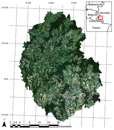
Figure 1.
The figure shows an overview of the study area. The background shows a RapidEye true color composite from 2016.
2.2. Classification Algorithms
The selection of algorithms to apply and validate in the presented study, is characterized by theoretical and practical considerations. The goal is to have a small set of both pixel based and convolution based classifiers, that give a realistic representation of classical as well as state of the art implementations in the field. The focus of this study is to provide conceptual considerations about model transferability, rather than developing and optimizing novel implementations. Thusly, for each modeling approach, one basic implementation, and one advanced iteration was selected (see also Table 1).

Table 1.
Overview of modeling algorithms.
Machine learning classifiers like Support Vector Machines and Random Forests have long been proven to be superior to statistical techniques like Maximum Likelihood (cf. [1]), and are well suited for binary land use classification tasks. Each single observation is a multivariate vector of independent variables, while the dependent variable is a binary outcome. Random Forest classifiers (cf. [30]) are particularly useful in the context of this study, because there are very few and mostly inconsequential hyperparameters required. It is a well established algorithm, and many different implementations exist. Within the context of this study, ranger was used, a well optimized and popular implementation of the random forest algorithm (cf. [31]). In addition to ranger, the Extreme Gradient Boosting (XGBoost, cf. [32]) algorithm was selected, to represent a more state of the art ensemble based machine learning method. It is very prominent in contemporary remote sensing studies (see [33,34]), well optimized for large datasets and implementations exist for R (cf. [35]). Both algorithms are representative for the two major resampling strategies in ensemble based machine learning, boosting and bagging [36,37]. Both aim to reduce variance in weak learners (i.e., single trees) by training many learners on resampled datasets, but boosting focusses more on reducing bias by iteratively adjusting new models to the residuals of the previous models [38].
In contrast to the aforementioned pixel based machine learning classifiers, Convolutional Neural Networks (CNN, cf. [39]) are able to derive arbitrary spatial features with kernel convolutions. With the rising popularity of deep learning algorithms since roughly 2016, they quickly saw widespread use in remote sensing applications, and are the most frequently applied deep learning algorithm by a big margin (cf. [21]). One simple way to implement a CNN is to stack many convoluted layers on top of each other, and merge them with a sigmoid activated fully connected output layer. This simple fully connected convolutional network (FCNN) is used as a baseline neural network in this study. It is implemented in keras (see [40]). A vast amount of neural network architectures have been developed and applied in the field of image analysis. In this study, the U-Net architecture (cf. [41]) has been chosen, because it is able to process geometric relationships on multiple levels. It has its origin in medical image segmentation, and uses a nested succession of downsampling with maxpooling layers, as well transposed convolutions to upsample to the original resolution again. Due to this varying and flexible implementation of scale, it is especially suited to make use of field geometries in large scale datasets.
Optimizing models in terms of tuning hyperparameters requires advanced strategies like grid search, which in turn rely on measuring validation performance. Since the main focus of this study is to illustrate that measuring validation performance is not trivial and involves a clear definition of scope, the same reasoning has to be applied when optimizing parameters for model tuning. The focus is not to optimize the performance of a model in a given scope, the focus is to compare performances of models when changing scope. Therefore, default hyperparameters were kept whenever possible. If not, models were optimized manually, by trying out different combinations on a larger subset in order to find parameters that give good training results. The ranger model performed well out of the box, and the default parameters (number of trees and number of variables in each split) were kept. The xgboost model comes with additional hyperparameters specific to the chosen booster. We were also able to keep the default parameters of the tree booster here, since they performed well on the training data.
Hyperparameter selection for deep learning algorithms is much more complicated, since they can have arbitrary complexity in the network architecture, while each part of the network can have parameters and functions to adjust. The shape of the input tensor is the first part of the architecture that needs to be defined, and is the same for both fcnn and unet. It is defined by the dimensions of the input dataset, and the edgesize of one sample cell. We decided to set the edgesize rather small, to keep the number of layers low. The edgesize has to have 2 as multiple factors to allow for downsampling in the unet algorithm, so 32 was chosen in both convolution based algorithms. The rest of the fcnn model is rather simple. In total, 20 convolution layers with rectified linear unit activation functions were found to be enough to segment the input images. These layers were then combined in a final sigmoid activated output layer. The unet model was initialized with 10 convolution layers before the first downsampling step, and four downsampling steps with 50% dropout layers total. In addition to the model specific hyperparameters, the training of a deep learning algorithm itself is defined by an additional set of parameters as well as the optimizer and the loss function. We again tested several approaches with a training subset of the study area and found that the very common RMSprop optimizer in combination with a binary crossentropy loss function worked well. Both models were then trained with a batch size of 10, for 150 epochs.
2.3. Data Sources
2.3.1. Reference Data
As a direct result of the common agricultural policy of the European Union, all administrative units are keeping track of field geometries and crops in their municipalities. The integrated administration and control system (InVeKos [42]) is used to register all official records, in exhaustive geodatasets. In this study, we use shapefiles from 2016 till 2019 each containing roughly 50,000 discrete field geometries. The field geometries have distinct registered crop types, of which around 100 different types exist in the area. Of these crop types, the ones that cover the different type of maize were selected, converted to a binary variable, and rasterized in a grid aligned to the image data (see Figure 2).
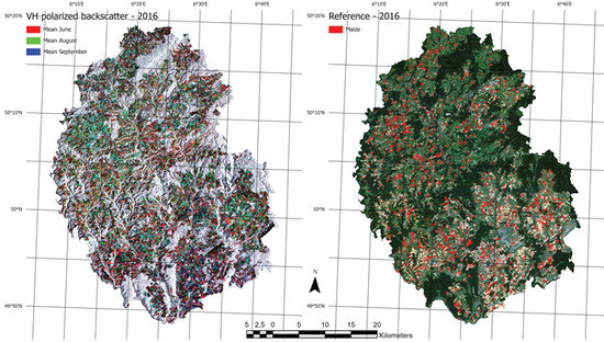
Figure 2.
The figure shows an overview of input data. The left side shows an RGB composite of three different monthly means from the Sentinel-1 input data. The right side shows a rasterized version of all maize fields from the the InVeKos dataset with a RapidEye RGB composite in the background.
2.3.2. Image Data
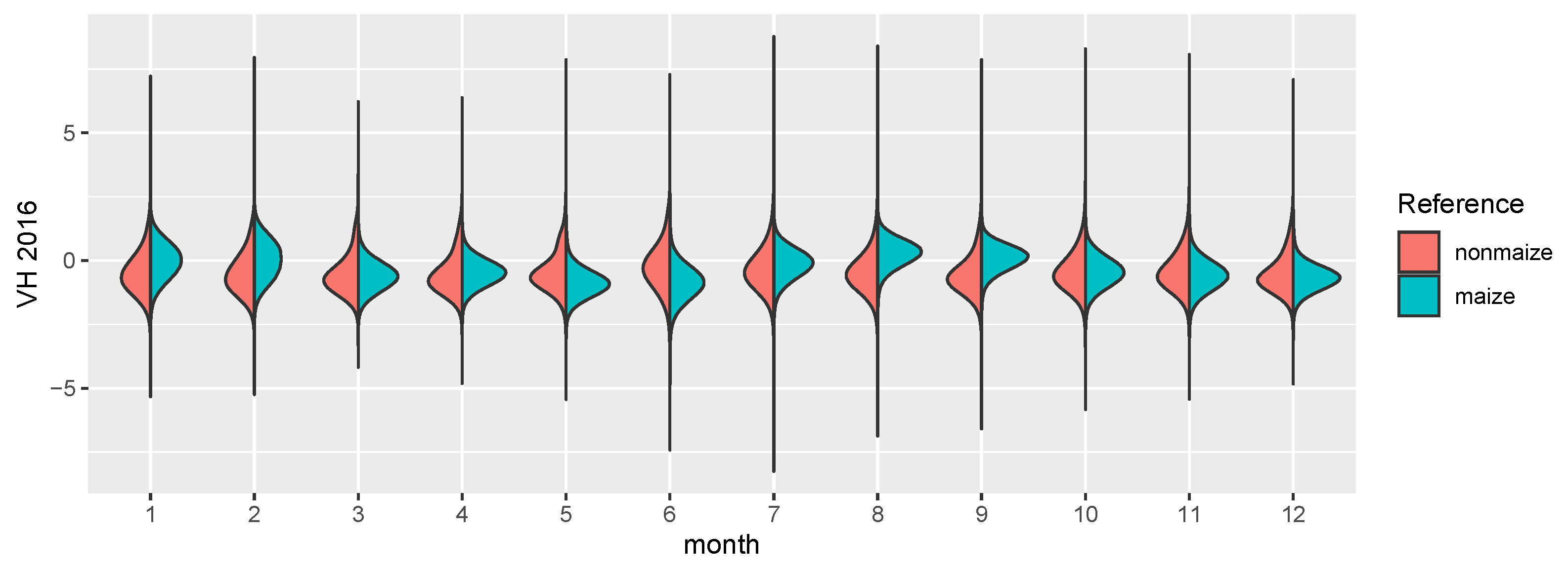
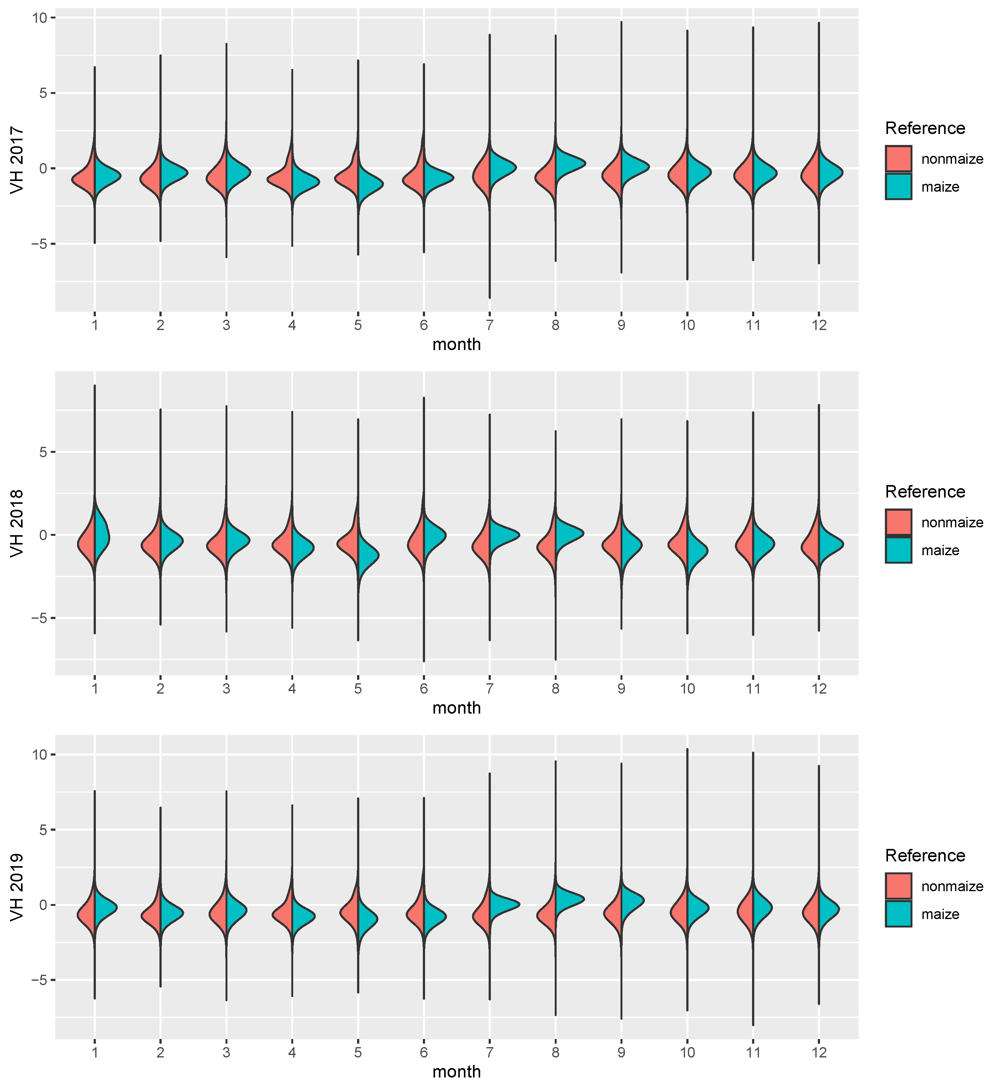
The focus of this study is the transferability of image based models on a regional scale, both temporally and spatially. Consequently, SAR imagery is well suited as a prediction input. While it is much harder to interpret visually and the signal of the phenology is not as clear as in the reflectances of a vegetation spectrum, it is largely unaffected by atmospheric conditions. While it is affected by topography and soil water content, monthly timeseries can be derived consistently, which show distinct temporal patterns for certain crop types [43]. Along with the benefit of temporal consistency, SAR imagery comes with other downsides, most importantly the complete lack of information about leaf pigments [22] and generally lower ground sampling distance (GSD). The sensor used in this study is the C-band SAR mounted on the Sentinel-1 satellites A and B. We used the ground range detected (GRD) product with the instrument mode interferometric wide swath. GRD imagery provides the advantage of speckle and noise reduction through multi-looking (5 looks in this case), at the cost of losing the phase information of the signal, as well as an increased GSD. We used the level 1 GRD high resolution product with vertical transmit/horizontal receive polarization, which has a GSD of 10 m [44]. VH crosspolarized SAR data benefits from the increasing interaction of transmitted and received waves, as the canopy height develops [45]. The data was processed in and downloaded from the google earth engine (GEE, cf. [46]). GEE Sentinel-1 datasets are pre-processed by the Sentinel-1 Toolbox, which means that thermal noise removal, radiometric calibration and terrain correction algorithms were applied. Since the Sentinel-1 constellation has a revisit time of roughly 6 days, and 12 days in 2016 because there was only Sentinel-1 A, monthly means could be computed for every single pixel. This lead to a consistent 12 band image with 10 m GSD for all 4 years. In a last step, each image was scaled. Figure 3 shows the distributions of both classes in the images. Though SAR is invariant to pigment features of the canopy, even on this aggregated level the growth curve of maize, starting around June and ending in September/October, is visible. One example year is visualized in Figure 2, where the maize fields have a distinct green/turquoise hue, which indicates a peak in Augst/September, as opposed to the red crops which are also visible.
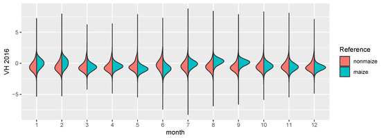
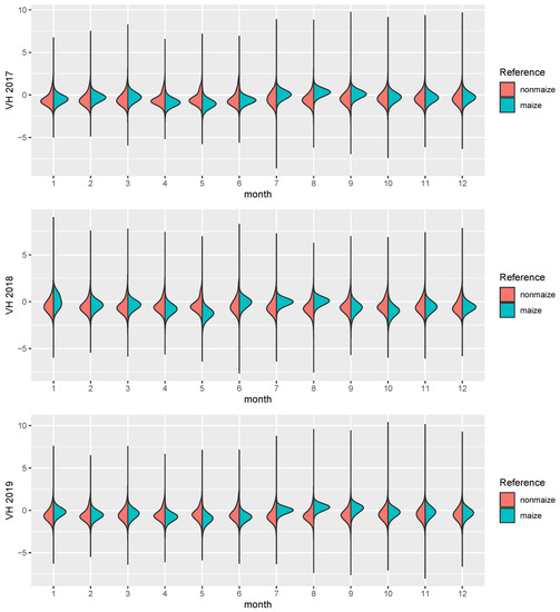
Figure 3.
The figure shows distribution density estimates of the 12 monthly means for 4 years, split by maize (turquoise) and nonmaize (red) pixels.
2.4. Research Design
2.4.1. Spatiotemporal Generalization
The basis of this study is a repeated resampling of 5 by 5 km tiles (500 by 500 pixels) by changing location within the Eifelkreis Bitburg-Prüm, and the year ranging from 2016–2019. One sample contains a total of 4 tiles, from two different locations (hereafter called m and k), and two different years (hereafter called year 1 and year 2). For each run, all models are trained based on tile m_1 (see Table 2). From this tile, 500 sample cells with 32 by 32 pixels are drawn, while overlap is explicitly allowed. The result is a 500 × 32 × 32 × 12 tensor that is used as an input for the deep learning models. Since the cell shape is irrelevant for the pixel based algorithms, the input is then reshaped into observation rows with 12 variables. As a consequence of the input cell overlap, a lot of the observations are identical, so the amount unique observations is much lower than 500 × 32 × 32. Based on this sample, the four models are trained and all four tiles are then predicted.

Table 2.
Overview of Validation Scopes.
For the pixel based models, this prediction is simple. Since each pixel is treated independently, it is just a prediction with 250,000 observations and 12 variables. The convolution based predictions are a bit more complex, since inputs are not pixels, but cells. To predict a complete tile, each pixel is treated as a corner pixel of a cell, which creates overlap for pixels that are not at the borders of a tile. The predictions are then averaged for each pixel based on the values of all cells including that given pixel. As a consequence, the input datasets for pixel based and convolution based methods are not directly comparable since the raw amount of input data is, by virtue of nature, much higher for the convolution based algorithms.
Each tile then represents one of four basic generalization scopes. Tile m_1 represents the training scope. It still has pixels not sampled in the actual training dataset, but they are in close proximity and from the same year. Tile k_1 represents spatial generalization. Its dataset is from the same year, but the field geometry is relatively independent. Tile m_2 is at the exact same location as m_1 but from a different year, and the validation scope is therefore called temporal. Field geometries are not always identical, but changes are very minor. Tile k_2 represents spatiotemporal validation, because it is different in both location and year.
2.4.2. Geometrical Generalization
Kernel convolutions, which are the basis of CNNs, compute artificial features based on a given neighborhood. This means, that features like angled edges and texture can be included in the semantic segmentation optimized by the perceptrons. These features can be summarized as “geometry” of the field, and add an entirely new set of information to an observation, that pixel based algorithms cannot include. This layer of information can be useful in the classification of agricultural fields, because they are often defined by long straight edges and comparatively similar in size. It can also be harmful in temporal generalization, because in a field with a very specific shape, crop types can change from year to year, while the shapes stay mostly the same.
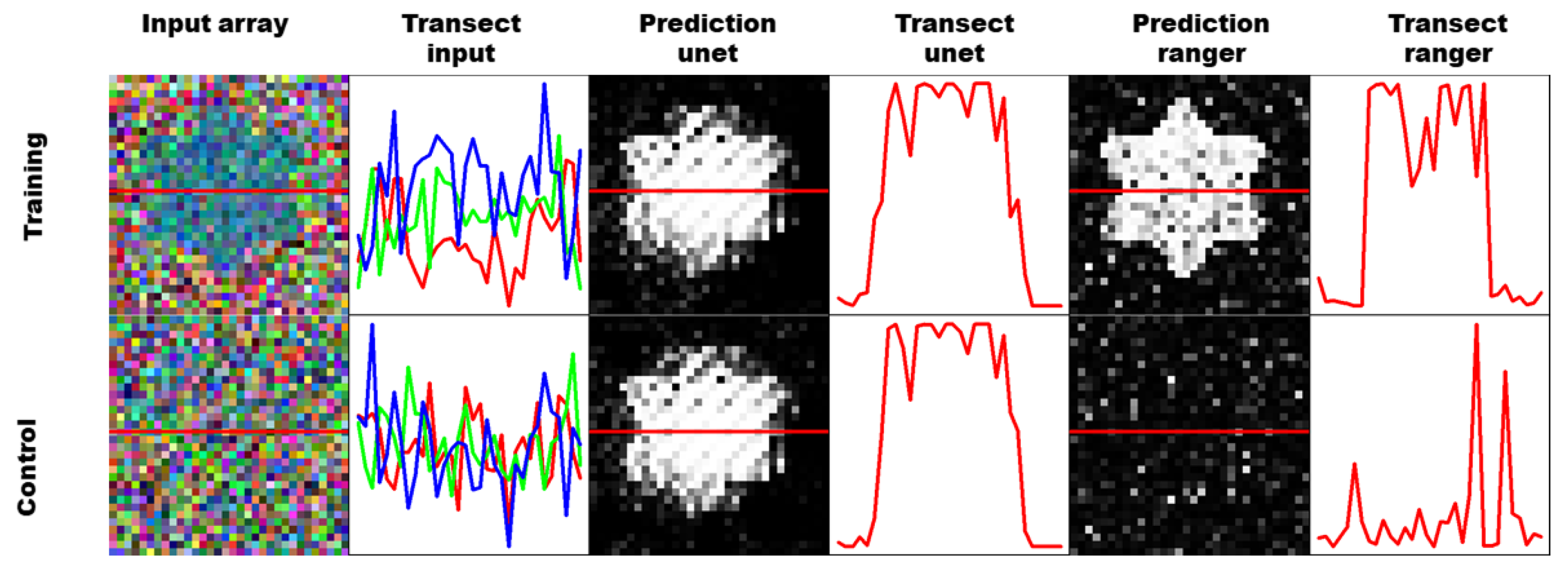
This problem is visualized in Figure 4, where training cells were artificially generated with a very specific star shape. Pixels that are known to be maize are randomly drawn from the image data and used to fill the star. Pixels that are known to be not maize are used to fill the rest of the cell, as well as an additional artificial control cell. The star shaped cells are then used to train a UNET CNN as well as a ranger classification model. The figure shows one prediction of a training cell, and a control cell for each classifier. The training prediction works well for both models, and the star shape is clearly visible. The control cell however, contains no pixels from maize fields, and the ranger classifier shows only a small amount of noise and misclassified pixels. The UNET classifier however, shows almost the exact same picture, which means that it was overfitting the geometry of the field, and seemingly did not include the numeric information of the pixel features at all.

Figure 4.
The figure is visualizing geometric overfitting by training based on an artificial sample with a star shaped maize field (top row) and validating on an artificial sample without maize (bottom row).
This artificial example is very far from field conditions, and overfitting of this kind would be easily detectable in simple crossvalidation or split-data validation samplings. It is still possible that the perceptrons could show a similar memory effect when trained on maize fields with unique geometric features. If the model is validated with spatial validation, just with image data from another location, this overfitting will not be apparent, because the classifier will never see the same shape again. If validated with temporal validation datasets, which contain the very same field from another year, the geometry will be the same, but the pixel features and potentially the crop type are different. A convolution based classifier could potentially be more likely to classify this as a maize field, because it has been trained to classify this geometry, albeit with different pixel features, as maize before. A pixel based classifier is invariant to the geometry, and therefore the classification result should not be biased.
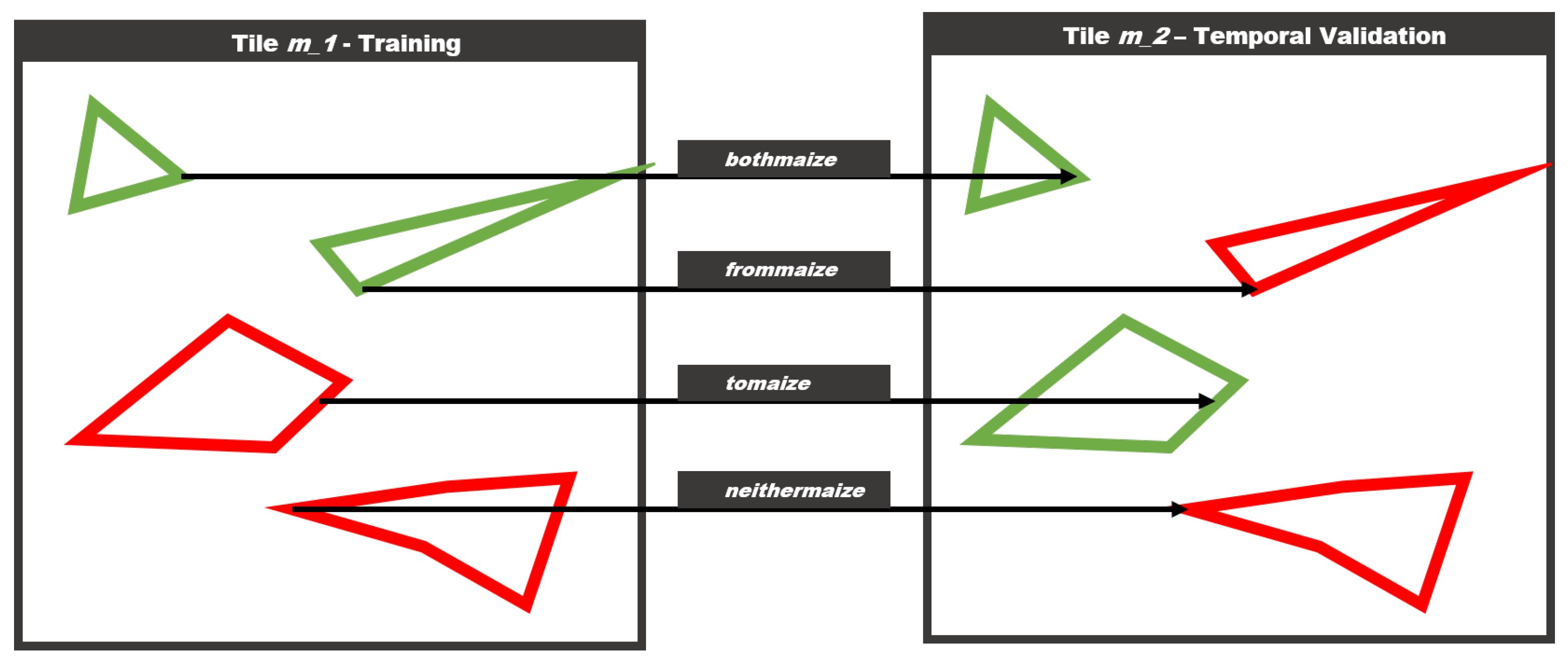
Resampling from a large dataset spanning an entire region for multiple years, provides the unique opportunity to specifically assess this kind of overfitting problems. Thusly, we introduce four additional scopes, that are a subset of the temporal scope defined in Table 2 since they only apply to tile m_2, which has the same geometry but data from a different year. One caveat of this approach is that the geometry between two years is not exactly the same. There are some differences between polygon geometries from all four years, but they are usually very minor, and this simplification should have little impact on the overall conclusion of the study. The scopes themselves are described in Figure 5. The scope bothmaize includes fields that have been maize in the training year, and still are maize in the validation year, while the scope frommaize includes fields that were maize, but are not anymore.
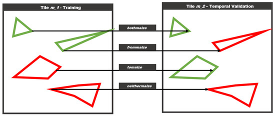
Figure 5.
The figure describes the geometric scopes for the validation approach. Assuming the same geometry in a different year, there are four possible scenarios.
The scope tomaize includes fields that have not been maize in the training year, and changed to maize in the validation year, while the scope neithermaize includes fields that are not maize in both the training and validation year. Conceptually the performances in the bothmaize and tomaize scopes should be similar, as well as the performances of frommaize and neithermaize.
2.4.3. Performance Metrics
Binary classification is a concept known in many different domains, and as such, a large amount of classification performance metrics exist. All of them have in common, that they are based on the confusion matrix (CM) (cf. [47]). Overall accuracy is a metric directly derived from the CM, but has the problem that it is misleading if the no information rate is high, i.e., if there is a large imbalance between the two classes. Other base metrics, like sensitivity/specificity and precision/recall give a better idea of the overall performance because they are not focused on the diagonal of the CM. Additionally, there are higher level metrics like Cohens kappa and the F1 score. Cohens kappa has been very popular in remote sensing publications in the past, but has been heavily criticized (cf. [23,48]). It has also the problem that it is a very domain specific metric, and implementations in contemporary deep learning frameworks is not common. In this study, F1 (see Table 2 and Table 3) will be used as a comprehensive and widespread higher level metric, in addition to the base metrics precision and recall. In some geometric scopes there are no true positives or negatives, therefore sensitivity and specificity will be reported if applicable.

Table 3.
Overview of Comparison Scopes.
In a final step, Mann–Whitney U-tests will be used to compare the performances of each model against each other. Since the metrics used range from 0 to 1, they are not normally distributed, therefore a nonparametric two sample test will be used to test the alternative, that a given test yields better results on average than the test it is compared against. Between the geometric scopes, two sided tests will be used in oder to test the null hypothesis that bothmaize and tomaize yield on average similar performances. In other words, that the sensitivity of maize fields is indifferent to the status of that particular field in training.
3. Results
3.1. Illustrative Sample Run
Figure 6 and Figure 7 show the input data of one sample run. Tile m shows a heterogenous landscape, structured by riverbeds and disperse forest areas. It has a moderate amount of maize fields compared to tile k, which shows a very high density of maize fields divided into small sections in the north, and a dense forest in the south. The fields in tile k are also very regularly shaped compared to the fields in tile m.

Figure 6.
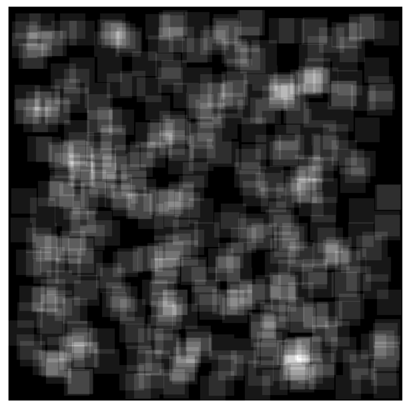
The figure shows the spatial distribution of training cells in a tile. A substantial amount of overlap is visible and necessary, since cells that contain the same field but slightly translated still provide new information to the classifiers. For the pixel based algorithms only unique pixels were counted, in this 207,595 observations, roughly 84% of the entire tile.
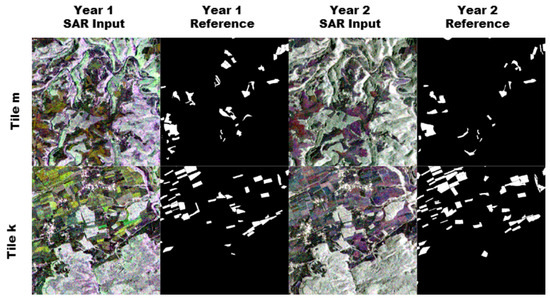
Figure 7.
The figure shows a sample for one complete run. The two rows show tile m and k. Columns 1 and 3 show false color composites of the 12 band monthly mean Sentinel-1 images. Columns 2 and 4 show the position of the maize pixels in white.
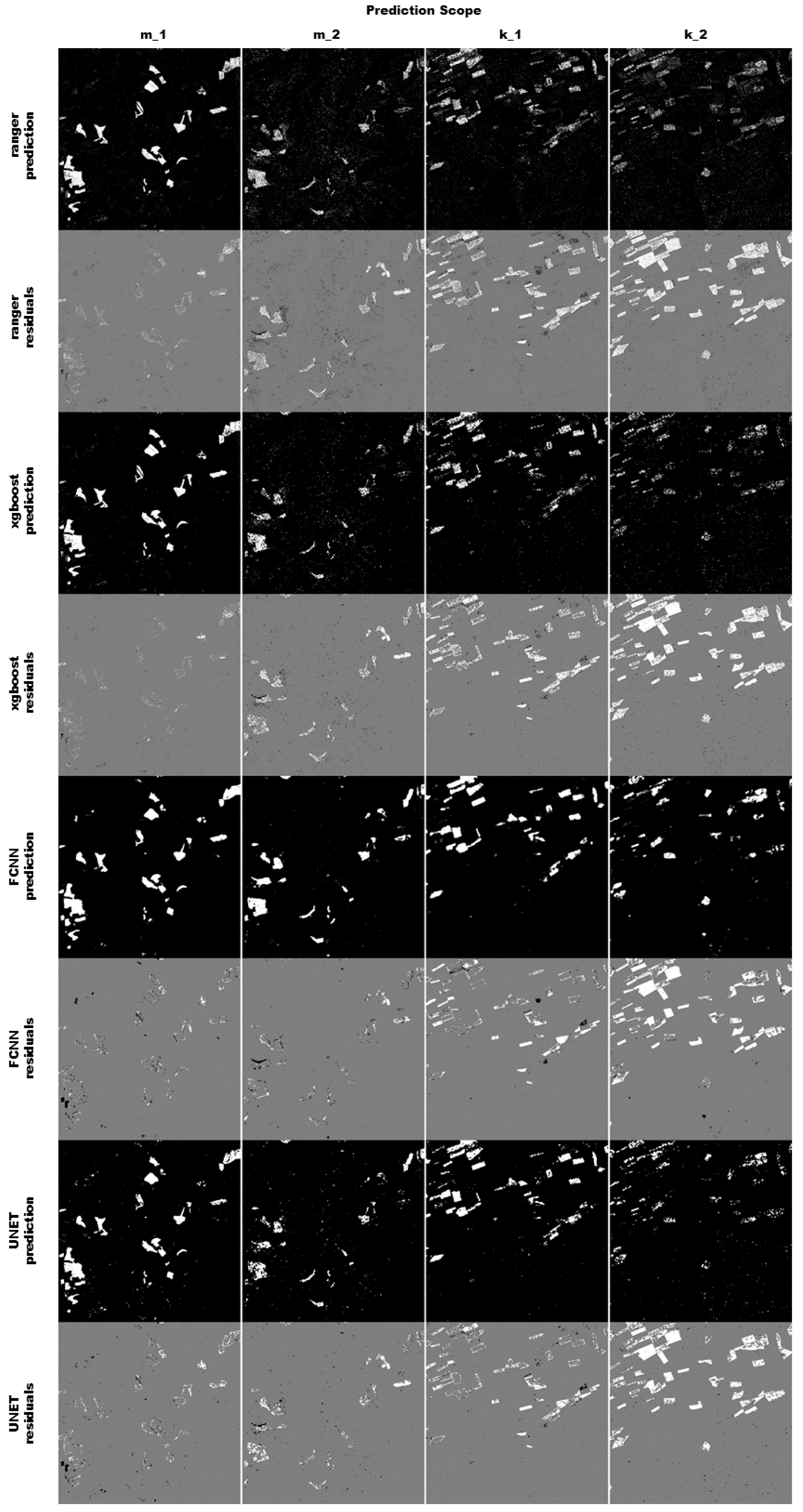
All four algorithms predicted the training tile m_1 rather well (see Figure 8), and did not miss any of the fields. The pixel based classifiers produce spatially rather evenly distributed residuals. The residuals produced by the convolution based algorithms are more clustered and are often missing entire fields or sections of fields. Sometimes the residuals of both FCNN and UNET form clearly structured spatial patterns around fields, indicating that the geometry of the reference data is slightly bigger than the prediction. Overall none of the four classifiers are able to adequately perform the binary segmentation in the second tile k, especially in the second year. However, there are some minor differences in how the classifiers predict, and it is not obvious which one performs better. To asses this, this random sample was repeated 500 times, and the results were summarized in the upcoming section.

Figure 8.
The figure shows a result for a complete run. The four different scopes are shown in the columns, while the model predictions and residuals are shown in the rows. The prediction pixels are colored in white (predicted to be maize) and black (predicted to be not maize). The residuals are colored in white (false negative), black (false positive) and grey (true positive or true negative).
3.2. Spatiotemporal Generalization
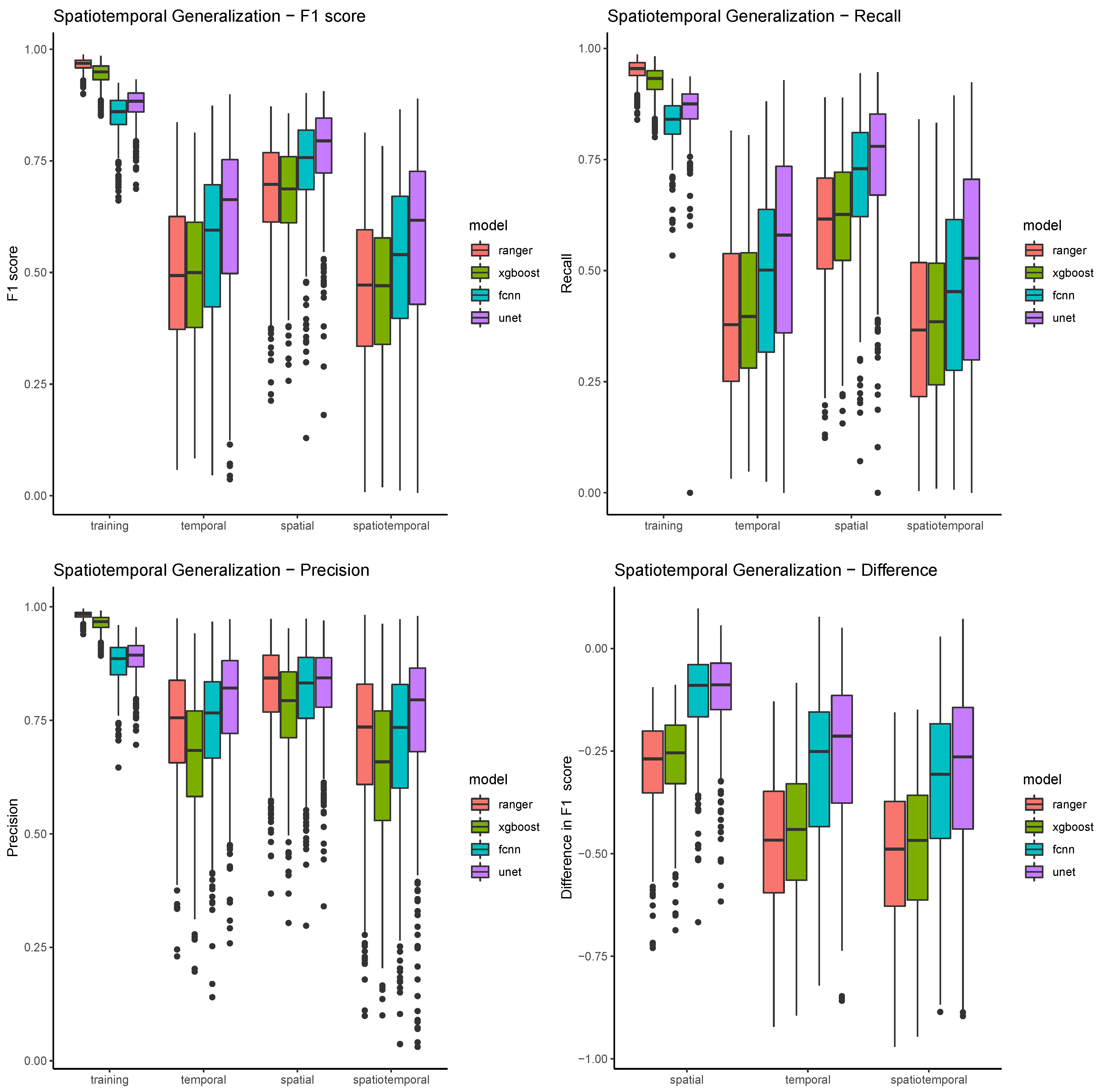
Table 4 and Figure 9 show the model summaries of all 500 resampling runs, grouped by algorithm and validation scope. They show a very clear pattern of differences for the four different scopes. In the training scope, all four classifiers are able to achieve relatively high F1 scores (mostly above 0.75), with relatively low standard deviations (below 0.05). In all the other scopes, performances are both much lower on average, and much more varied. The spatial scope has still relatively high scores, ranging from 0.68 (ranger) to 0.77 (UNET), and also much higher standard deviations. The temporal validation scopes show even lower performances, while spatiotemporal scopes show the lowest overall performances, and the highest variability. In general, the true positive rate, or recall, seems to be a big problem in most models. While still above 0.9 for the pixel based models, and above 0.8 for the convolution based models, the detection rates drop mostly below 0.5 in the temporal and spatiotemporal validation scopes (see Table 5). The algorithm ranger detects on average just about one third (36.6%) of maize pixels in the spatiotemporal validation scope. Precision rates (see Table 6) in comparison are much higher, and also much less variable within models, between models, and between scopes. This means that false positives are rather uncommon with all four classifiers (see also Figure 8). XGBoost seems to have the highest false positive rate, and performs considerably worse than the other classifiers, and ranger in particular.

Table 4.
Summary Spatiotemporal Generalization—F1.
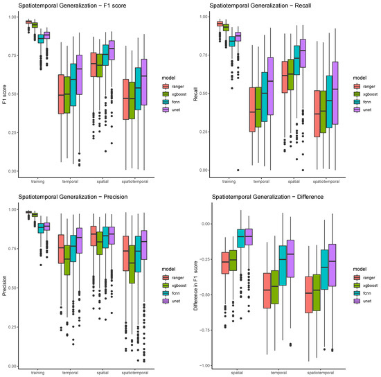
Figure 9.
The figure shows boxplots for all three performance metrics plus the performance difference between scopes. Boxplots are grouped by scope and colored by model.

Table 5.
Summary Spatiotemporal Generalization—Recall.

Table 6.
Summary Spatiotemporal Generalization—Precision.
The same pattern, spatial generalization being better than temporal, and temporal generalization being better than spatiotemporal, can be observed when just looking at the differences in scores (see Figure 9). The validation score differences show, compared to the absolute performance scores, relatively low standard deviations. Both pixel based methods and both convolution based methods show similar value ranges in the spatial comparison scope, with convolution based methods losing much less performance. The performance difference in the temporal and spatiotemporal validation is much higher, and the difference between all models gets more pronounced.
The statistical analysis in Table 7 shows that ranger is the superior classifier in the training scope, and both pixel based classifiers are significantly better than the convlution based models. In all other scopes, the convolution based classifiers perform significantly better, with UNET being the most accurate of them. The difference between ranger and xgboost is much less significant, than the difference between UNET and xgboost.

Table 7.
Summary of Mann–Whitney U tests.
3.3. Geometric Generalization
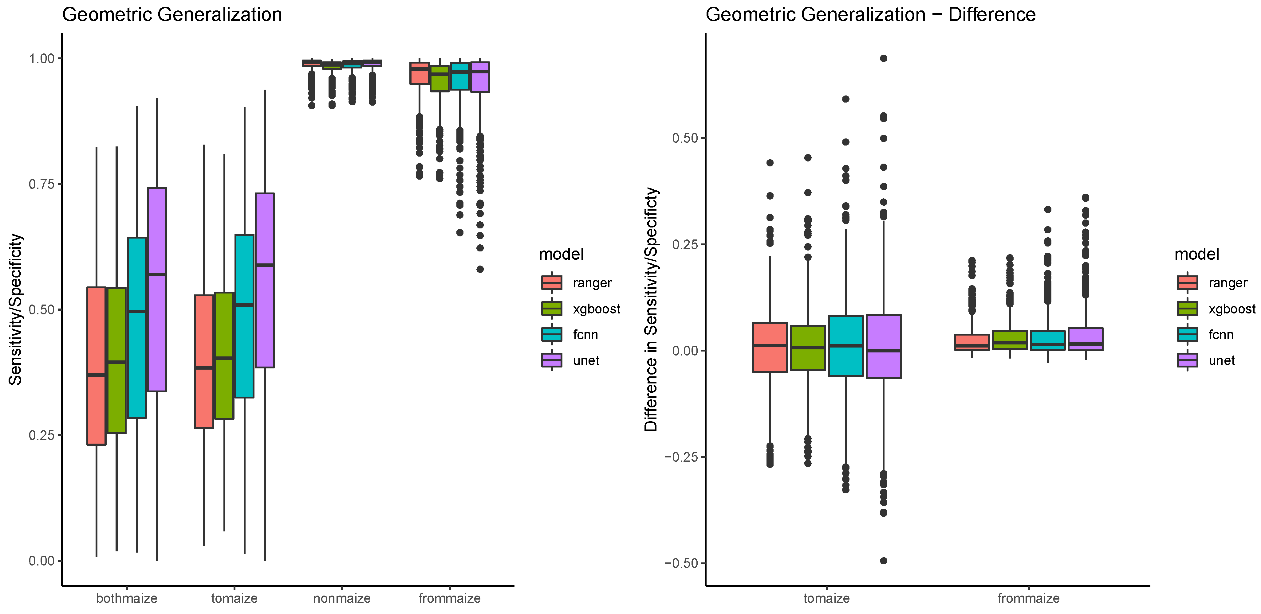
Figure 10 shows that the patterns established in the spatiotemporal generalization also appear in sensitivity performances in maize fields, with the pixel based classifiers being relatively similar, FCNN being much better, and UNET outperforming all of them. At the same time, the value ranges and medians of the performances are very similar for the scopes bothmaize and tomaize. The value ranges of the scopes nonmaize and frommaize are relatively low, but nonmaize shows a much smaller variability, and a much more consistent specificity (see also Table 8). From the geometric validation scopes, nonmaize is special in a way that it is the only scope that contains pixels that are not agricultural. The fraction of these pixels is rather high (around 87% in comparison to 3/5/5% for bothmaize/tomaize/frommaize), and they are at the same time much easier to discriminate. Looking at differences between the algorithms, the specificity values show very little difference, mostly because most values are consistently high. The right side of Figure 10 summarizes the performance metrics by calculating the differences in performance for maize pixels (to maize) and nonmaize pixels (from maize). This difference is around 0 in all cases, with again higher variance in the sensitivities compared to the specificities.
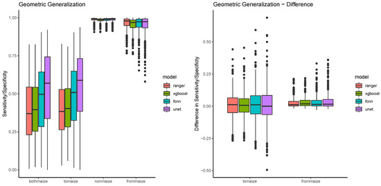
Figure 10.
The figure shows a boxplot for the performance difference between scopes colored by model.

Table 8.
Overview of Spatiotemporal Generalization Scopes.
The statistical analysis (see Table 9) verifies that there is no significant difference between the bothmaize and tomaize scope. This means, that none of the four classifiers of maize fields is biased by the status of the field in the training year. If a field is maize in the training year, its not more or less likely to be detected in the validation year than a field that is not maize in the training year. On the other hand, the analysis shows significant differences between the nonmaize and frommaize scope. This is again due to the fact that nonmaize is special because of a much larger variety of pixels. The scope signifiance is however relatively consistent for all four models.

Table 9.
Summary of Mann–Whitney U tests—geoscopes.
4. Discussion
4.1. Input Data
The focus of this study was to assess advantages of convolution based models in model generalization. To find and optimize a novel combination of deep learning model and multitemporal image data was outside of the scope of this study. Thusly, some simplifications have been made which provide ample opportunity to improve the absolute performances of the models, while at the same time preserving the relative differences between the validation scopes. The Sentinel-1 imagery was processed out the box and monthly averages were calculated. Improvements to data quality can be largely categorized in three groups, noise reduction, adding information and reducing redundancy. Thermal noise removal is already implemented in the Sentinel-1 Toolbox, but bias introduced by different incidence angles could be corrected with empirical coefficients. Information could simply be added, either from the same sensor but with a different cross-polarization mode, or from other sensors with high revisit times like Sentinel-2. Furthermore and within the SAR domain, data preprocessing algorithms like polarimetric decomposition could be used to gain more information about the exact nature of the scattering. Furthermore, finally, redundancy could be reduced with data transformation algorithms like the principal component analysis or even implemented in the deep learning framework itself with autoencoders.
One major caveat is that the drop in sensitivity/recall rates in all the validation scopes was very high for most models. However, two counterpoints suggest that this is a modeling problem and not an input data problem. First, the variability with a given model is high, which indicates a strong random effect of tile selection, for both validation and training tiles. Furthermore, high variability means that there is still a lot of potential to increase model sensitivities by increasing the size of training datasets, which is easily possible by several orders of magnitude. Secondly, the variability between models is very high, which in a similar way suggest that there is potential to delineate maize fields, which could be developed with further algorithm Improvements. As a consequence it can be concluded that SAR imagery provides a good basis for temporally and spatially transferable crop classification models.
4.2. Validation Scopes
Validating within the training scope is the most common step of each modeling process, and for deep learning algorithms even required in each iteration as part of the loss function. High performance in the training scope is necessary for each model, but not a sufficient criterion for a useful model in most research contexts. All models in this study were able to achieve reasonably high performances in the training scope, but the spatiotemporal scopes were able to show a much more complete picture. Here, the convolution based algorithms performed better by a very significant margin.
Changing the location or year of a sample is a simplification for changing the many factors that result in a different phenology with the same crop type. These factors can be anything, from different altitudes and microclimate in neighboring regions, different precipitation and drought patterns in two years, to different management practices of two farmers in fields right next to each other. Ideally, we would have complete spatial information about all of them, and we would do a stratified sampling based on altitude, water availability and crop management. While altitude and precipitation strata could be implemented, crop management variables are nearly impossible to get for larger datasets and multiple years. Furthermore, there are many more variables that needed to be accounted for in a stratified sampling. Some of these factors are more likely to be different in different years, while some of them are more likely to be different in different locations. Consequently, changing both allows for a more complete assessment of model performance, without the requirement of other spatial datasets necessary for a stratified sampling, a concept that can be easily applied to other crop classification studies.
The geometric scopes however, are most likely not very useful in other contexts. They were only included to analyse a very specific aspect of convolution based classifiers, and were not able to lead to any further conclusions. Potential overfitting and memory problems could be also analysed with spatial validation scopes, but geometric scopes were more precise in that regard.
4.3. Model Training and Evaluation
Since optimizing the absolute performance of the models was not the focus of the study, the pixel based models in this study were trained with default hyperparameters wherever possible, and it is expected that the impact on their performance is very low. The same cannot be said about the convolution based models, where model performance can be optimized by many different parameters, activation functions, choosing the right optimizer and adjusting the network architecture. Wherever possible default parameters were used, but there is without a doubt a lot of potential to find better models than the ones used in this study. This does not affect the findings, but could in the future be used to build on the validation framework established in this study.
Despite this limitation, we were able to show, that models are much more performant if applied to different regions than compared to different years. In SAR remote sensing, there are less reasons to assume this would be the case, compared to optical remote sensing where the image acquisition is very time critical and sporadic because of atmospheric constraints that apply much less to radar data. Instead we have consistent monthly means that cover the entire year and are largely invariant to atmospheric conditions. However, the phenology development curve is still potentially very different in different years because of precipitation and sunlight. Additionally, there might be SAR specific factors that cause short term fluctuations of the backscatter coefficients. Surface wetness, for example, can cause short term spikes in VH backscatter of vegetation coverage [49]. Because of these uncertainties, it is unclear if this particular finding can be transferred to other crop classification applications. It is however, evidence that spatial validation (i.e., randomized samples from one year) gives an incomplete picture of model transferability.
In addition we provide evidence that including field geometry (i.e., with convolutional neural networks) is beneficial to model generalization. Pixel based models, while being consistently more performant in the training subset, showed clearly less sensitivity to maize pixels than the convolution based models, while at the same time being unable to offer more precision as a tradeoff. Geometric overfitting has been shown to not be a problem in any of the models. Though it cannot be ruled out that geometry based memory effects could happen in certain models, there is still enough evidence that convolution based models generalize much better, and it is hard to imagine future crop classification research without it.
5. Conclusions
- SAR imagery provides a good basis for temporally and spatially transferable crop classification models
Despite the simplifications made in the preprocessing of the datasets, and despite the fact that it is also affected by topography and soil wetness, the information represented by the SAR imagery was shown to be sufficient to detect between 95% (ranger) and 85% (UNET) of maize fields in the training scope. The main benefits is independence from atmospheric conditions and consistently available image products as a result. The main drawback is insensitivity to leaf pigments, and therefore major limitiations in other aspects of vegetation monitoring.
- Within a region, temporal generalization is harder than spatial generalization.
Most studies in the past have focused on spatial validation by splitting their training datasets. With freely available datasets and a growing body of highly capable classifiers, temporal generalization is a designated goal for a growing body of LULC classification research. We were able to highlight the importance of temporal validation, by showing that there was a significant drop in model quality if a model was validated with data from a different year, compared to data from a different region. F1 scores dropped to values between 0.49 (xgboost) and 0.61 (UNET) in the temporal validation scope, compared to values between 0.67 (xgboost) an 0.77 (UNET).
- Validation scopes can be helpful in assessing model quality
Analyzing these models showed that a comparatively high modeling performance was achieved within the training scope, even though the amount of training samples was relatively low. Switching scopes gave a much more complete picture. By analyzing the drop in performance observed when validating with samples from these different scopes, some algorithms were shown to be significantly more robust, even though their performance in the training scope lower. Therefore, the concept of validation scopes has been proven to be a helpful tool in assessing the quality of a model.
- Including field geometry is helpful and geometric overfitting is not a problem
The main goal of this study was to compare classical machine learning classifiers to state of the art deep learning algorithms. By using a robust harmonized dataset for these years, as well as a randomized, scope based sampling approach, we were able to show that convolution based algorithms are clearly superior to pixel based algorithms. Albeit none of the tested algorithms in this study was able to produce a well generalizable classifier, it was shown that kernel based convlutions showed much more promise, and have potential to be a stable entity in all future crop classification research.
Author Contributions
Conceptualization, M.G.; methodology, M.G.; software, M.G.; validation, M.G.; writing—original draft preparation, M.G.; writing—review and editing, M.G. and T.U.; visualization, M.G.; supervision, T.U.; All authors have read and agreed to the published version of the manuscript.
Funding
This research received no external funding.
Acknowledgments
Thorsten Ruf for general ideas and background info, Daniel Bersch from the Statistical Office of the Federal State Rhineland-Palatinate for providing the agricultural records. Planet Labs Germany and the German Aerospace Center for providing RapidEye satellite images.
Conflicts of Interest
The authors declare no conflict of interest.
Abbreviations
The following abbreviations are used in this manuscript:
| CNN | Convolutional Neural Network |
| RF | Random Forest |
| masl | meters above sea level |
| FCNN | Fully Convolutional Neural Network |
| SAR | Synthetic Aperture Radar |
| GSD | Ground Sampling Distance |
| GRD | Ground Range Detected |
| CM | Confusion Matrix |
References
- Khatami, R.; Mountrakis, G.; Stehman, S.V. A meta-analysis of remote sensing research on supervised pixel-based land-cover image classi fi cation processes: General guidelines for practitioners and future research. Remote Sens. Environ. 2016, 177, 89–100. [Google Scholar] [CrossRef]
- Song, X.-P.; Huang, W.; Hansen, M.C. An evaluation of Landsat, Sentinel-2, Sentinel-1 and MODIS data for crop type mapping. Sci. Remote Sens. 2021, 102560. [Google Scholar] [CrossRef]
- Yuan, X.; Shi, J.; Gu, L. A review of deep learning methods for semantic segmentation of remote sensing imagery. Exp. Syst. Appl. 2021, 169, 114417. [Google Scholar] [CrossRef]
- Wang, S.; Chen, W.; Xie, S.M.; Azzari, G.; Lobell, D.B. Weakly supervised deep learning for segmentation of remote sensing imagery. Remote Sens. 2020, 12, 207. [Google Scholar] [CrossRef]
- Lavreniuk, M.; Kussul, N.; Novikov, A. Deep learning crop classification approach based on sparse coding of time series of satellite data. In Proceedings of the International Geoscience and Remote Sensing Symposium (IGARSS), Valencia, Spain, 22–27 July 2018; pp. 4812–4815. [Google Scholar] [CrossRef]
- Zhang, D.; Pan, Y.; Zhang, J.; Hu, T.; Zhao, J.; Li, N.; Chen, Q. A generalized approach based on convolutional neural networks for large area cropland mapping at very high resolution. Remote Sens. Environ. 2020, 247, 111912. [Google Scholar] [CrossRef]
- Rustowicz, R.; Cheong, R.; Wang, L.; Ermon, S.; Burke, M.; Lobell, D. Semantic Segmentation of Crop Type in Africa: A Novel Dataset and Analysis of Deep Learning Methods. In Proceedings of the CVPR Workshops, Long Beach, CA, USA, 16–20 June 2019; Volume 1, pp. 75–82. [Google Scholar]
- Harfenmeister, K.; Itzerott, S.; Weltzien, C.; Spengler, D. Agricultural Monitoring Using Polarimetric Decomposition Parameters of Sentinel-1 Data. Remote Sens. 2021, 13, 575. [Google Scholar] [CrossRef]
- Parida, B.R.; Mandal, S.P. Polarimetric decomposition methods for LULC mapping using ALOS L-band PolSAR data in Western parts of Mizoram, Northeast India. SN Appl. Sci. 2020, 2. [Google Scholar] [CrossRef]
- Sonobe, R. Parcel-based crop classification using multi-temporal TerraSAR-X dual polarimetric data. Remote Sens. 2019, 11, 1148. [Google Scholar] [CrossRef]
- Kussul, N.; Lavreniuk, M.; Skakun, S.; Shelestov, A. Deep Learning Classification of Land Cover and Crop Types Using Remote Sensing Data. IEEE Geosci. Remote Sens. Lett. 2017, 14, 778–782. [Google Scholar] [CrossRef]
- Wei, S.; Zhang, H.; Wang, C.; Xu, L.; Wu, F.; Zhang, B. Large-scale rice mapping of Thailand using sentinel-1 multi-temporal SAR data. In Proceedings of the 2019 SAR in Big Data Era, BIGSARDATA 2019, Beijing, China, 5–6 August 2019. [Google Scholar] [CrossRef]
- Xu, J.; Zhu, Y.; Zhong, R.; Lin, Z.; Xu, J.; Jiang, H.; Huang, J.; Li, H.; Lin, T. DeepCropMapping: A multi-temporal deep learning approach with improved spatial generalizability for dynamic corn and soybean mapping. Remote Sens. Environ. 2020, 247, 111946. [Google Scholar] [CrossRef]
- Kumar, P.; Gupta, D.K.; Mishra, V.N.; Prasad, R. Comparison of support vector machine, artificial neural network, and spectral angle mapper algorithms for crop classification using LISS IV data. Int. J. Remote Sens. 2015, 36, 1604–1617. [Google Scholar] [CrossRef]
- Skakun, S.; Kussul, N.; Shelestov, A.Y.; Lavreniuk, M.; Kussul, O. Efficiency Assessment of Multitemporal C-Band Radarsat-2 Intensity and Landsat-8 Surface Reflectance Satellite Imagery for Crop Classification in Ukraine. IEEE J. Sel. Top. Appl. Earth Obs. Remote Sens. 2016, 9, 3712–3719. [Google Scholar] [CrossRef]
- Castro, J.D.B.; Feitoza, R.Q.; Rosa, L.C.L.; Diaz, P.M.A.; Sanches, I.D.A. A Comparative Analysis of Deep Learning Techniques for Sub-Tropical Crop Types Recognition from Multitemporal Optical/SAR Image Sequences. In Proceedings of the 30th Conference on Graphics, Patterns and Images, SIBGRAPI 2017, Niterói, Brazil, 17–20 October 2017; pp. 382–389. [Google Scholar] [CrossRef]
- Cai, Y.; Guan, K.; Peng, J.; Wang, S.; Seifert, C.; Wardlow, B.; Li, Z. A high-performance and in-season classification system of field-level crop types using time-series Landsat data and a machine learning approach. Remote Sens. Environ. 2018, 210, 35–47. [Google Scholar] [CrossRef]
- Momm, H.G.; ElKadiri, R.; Porter, W. Crop-type classification for long-term modeling: An integrated remote sensing and machine learning approach. Remote Sens. 2020, 12, 449. [Google Scholar] [CrossRef]
- Ajadi, O.A.; Barr, J.; Liang, S.z.; Ferreira, R.; Kumpatla, S.P. Large-scale crop type and crop area mapping across Brazil using synthetic aperture radar and optical imagery. Int. J. Appl. Earth Obs. Geoinf. 2021, 97, 102294. [Google Scholar] [CrossRef]
- Zhu, X.X.; Tuia, D.; Mou, L.; Xia, G.S.; Zhang, L.; Xu, F.; Fraundorfer, F. Deep learning in remote sensing: A review. IEEE Geosci. Remote Sens. Mag. 2017. [Google Scholar] [CrossRef]
- Ma, L.; Liu, Y.; Zhang, X.; Ye, Y.; Yin, G.; Johnson, B.A. Deep learning in remote sensing applications: A meta-analysis and review. ISPRS J. Photogramm. Remote Sens. 2019, 152, 166–177. [Google Scholar] [CrossRef]
- Orynbaikyzy, A.; Gessner, U.; Conrad, C. Crop type classification using a combination of optical and radar remote sensing data: A review. Int. J. Remote Sens. 2019, 40, 6553–6595. [Google Scholar] [CrossRef]
- Olofsson, P.; Foody, G.M.; Herold, M.; Stehman, S.V.; Woodcock, C.E.; Wulder, M.A. Good practices for estimating area and assessing accuracy of land change. Remote Sens. Environ. 2014, 148, 42–57. [Google Scholar] [CrossRef]
- Pax-Lenney, M.; Woodcock, C.E.; Macomber, S.A.; Gopal, S.; Song, C. Forest mapping with a generalized classifier and Landsat TM data. Remote Sens. Environ. 2001, 77, 241–250. [Google Scholar] [CrossRef]
- Wolpert, D.H.; Macready, W.G. No Free Lunch Theorems for Optimization. IEEE Trans. Evol. Comput. 1997, 1, 67–82. [Google Scholar] [CrossRef]
- Su, T.; Zhang, S. Local and global evaluation for remote sensing image segmentation. ISPRS J. Photogramm. Remote Sens. 2017, 130, 256–276. [Google Scholar] [CrossRef]
- Ruf, T.; Gilcher, M.; Emmerling, C.; Udelhoven, T. Implications of Bioenergy Cropping for Soil: Remote Sensing Identification of Silage Maize Cultivation and Risk Assessment Concerning Soil Erosion and Compaction. Land 2021, 10, 128. [Google Scholar] [CrossRef]
- Gilcher, M.; Ruf, T.; Emmerling, C.; Udelhoven, T. Remote sensing based binary classification of maize. Dealing with residual autocorrelation in sparse sample situations. Remote Sens. 2019, 11, 2172. [Google Scholar] [CrossRef]
- Statistical Office Rhineland-Palatinate. Statistisches Jahrbuch Rheinland-Pfalz 2017. 2017. Available online: www.statistik.rlp.de/fileadmin/dokumente/jahrbuch/Jahrbuch2017.pdf (accessed on 19 February 2021).
- Breiman, L. Random forests. Mach. Learn. 2001, 45, 5–32. [Google Scholar] [CrossRef]
- Wright, M.N.; Ziegler, A. Ranger: A Fast Implementation of Random Forests for High Dimensional Data in C++ and R. J. Stat. Softw. 2017, 77, 1–17. [Google Scholar] [CrossRef]
- Chen, X.; Yin, D.; Chen, J.; Cao, X. Effect of training strategy for positive and unlabelled learning classification: Test on Landsat imagery. Remote Sens. Lett. 2016, 7, 1063–1072. [Google Scholar] [CrossRef]
- Saini, R.; Ghosh, S.K. Crop classification in a heterogeneous agricultural environment using ensemble classifiers and single-date Sentinel-2A imagery. Geocarto Int. 2019, 1–19. [Google Scholar] [CrossRef]
- Memon, N.; Patel, S.B.; Patel, D.P. Comparative Analysis of Artificial Neural Network and XGBoost Algorithm for PolSAR Image Classification; Springer: Cham, Switzerland, 2019; Volume 1941, pp. 452–460. [Google Scholar] [CrossRef]
- Chen, T.; Guestrin, C. Xgboost: A scalable tree boosting system. In Proceedings of the 22nd ACM SIGKDD International Conference on Knowledge Discovery and Data Mining, ACM, San Francisco, CA, USA, 13–17 August 2016. [Google Scholar]
- Saini, R.; Ghosh, S.K. Ensemble classifiers in remote sensing: A review. In Proceedings of the IEEE International Conference on Computing, Communication and Automation (ICCCA 2017), Greater, Noida, 5–6 May 2017; pp. 1148–1152. [Google Scholar] [CrossRef]
- Briem, G.J.; Benediktsson, J.A.; Sveinsson, J.R. Multiple classifiers applied to multisource remote sensing data. IEEE Trans. Geosci. Remote Sens. 2002, 40, 2291–2299. [Google Scholar] [CrossRef]
- Ribeiro, M.H.D.M.; dos Santos Coelho, L. Ensemble approach based on bagging, boosting and stacking for short-term prediction in agribusiness time series. Appl. Soft Comput. J. 2020, 86, 105837. [Google Scholar] [CrossRef]
- Lecun, Y.; Bottou, L.; Bengio, Y.; Haffner, P. Gradient-based learning applied to document recognition. Proc. IEEE 1998, 86, 2278–2324. [Google Scholar] [CrossRef]
- Allaire, J.J.; Chollet, F. Keras: R Interface to ’Keras’. 2020. Available online: https://cran.r-project.org/web/packages/keras/index.html (accessed on 19 February 2021).
- Falbel, D.; Zak, K. U-Net: Convolutional Networks for Biomedical Image Segmentation. 2020. Available online: https://github.com/r-tensorflow/unet (accessed on 19 February 2021).
- Federal Ministry of Justice and Consumer Protection. InVeKoSV. Available online: https://www.gesetze-im-internet.de/invekosv_2015/index.html (accessed on 19 February 2021).
- Veloso, A.; Mermoz, S.; Bouvet, A.; Le Toan, T.; Planells, M.; Dejoux, J.F.; Ceschia, E. Understanding the temporal behavior of crops using Sentinel-1 and Sentinel-2-like data for agricultural applications. Remote Sens. Environ. 2017, 199, 415–426. [Google Scholar] [CrossRef]
- Aulard-Macler, M. Sentinel-1 Product Definition. 2012. Available online: https://sentinels.copernicus.eu/documents/247904/1877131/Sentinel-1-Product-Definition.pdf/6049ee42-6dc7-4e76-9886-f7a72f5631f3?t=1461673251000 (accessed on 19 February 2021).
- Prudente, V.H.R.; Oldoni, L.V.; Vieira, D.C.; Cattani, C.E.V.; Del’Arco Sanches, I. Relationship between SAR/Sentinel-1 polarimetric and interferometric data with biophysical parameters of agricultural crops. Int. Arch. Photogramm. Remote Sens. Spat. Inf. Sci. ISPRS Arch. 2019, 42, 599–607. [Google Scholar] [CrossRef]
- Gorelick, N.; Hancher, M.; Dixon, M.; Ilyushchenko, S.; Thau, D.; Moore, R. Google Earth Engine: Planetary-scale geospatial analysis for everyone. Remote Sens. Environ. 2017. [Google Scholar] [CrossRef]
- Canbek, G.; Temizel, T.T.; Sagiroglu, S.; Baykal, N. Binary classification performance measures/metrics: A comprehensive visualized roadmap to gain new insights. In Proceedings of the 2nd International Conference on Computer Science and Engineering (UBMK 2017), Antalya, Turkey, 5–8 October 2017; pp. 821–826. [Google Scholar] [CrossRef]
- Pontius, R.G.; Millones, M. Death to Kappa: Birth of quantity disagreement and allocation disagreement for accuracy assessment. Int. J. Remote Sens. 2011, 32, 4407–4429. [Google Scholar] [CrossRef]
- Molijn, R.A.; Iannini, L.; Dekker, P.L.; Magalhães, P.S.G.; Hanssen, R.F. Vegetation Characterization through the Use of Precipitation-Affected SAR Signals. Remote Sens. 2018, 77, 1–17. [Google Scholar] [CrossRef]
Publisher’s Note: MDPI stays neutral with regard to jurisdictional claims in published maps and institutional affiliations. |
© 2021 by the authors. Licensee MDPI, Basel, Switzerland. This article is an open access article distributed under the terms and conditions of the Creative Commons Attribution (CC BY) license (http://creativecommons.org/licenses/by/4.0/).


