
Application of Sentinel-1 and-2 Images in Measuring the Deformation of Kuh-e-Namak (Dashti) Namakier, Iran

 ,
,
Abstract
:1. Introduction
2. Background
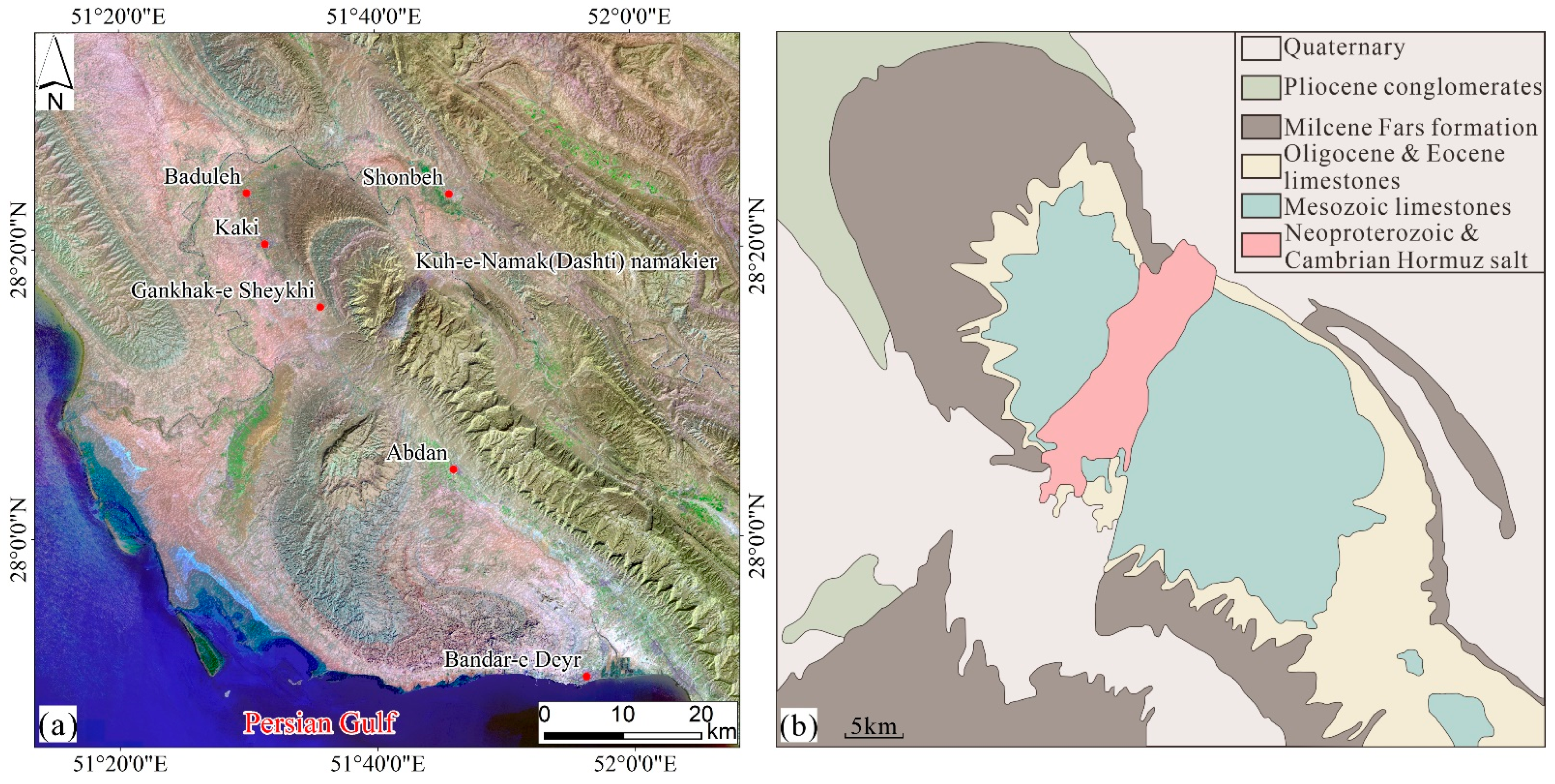
2.1. Geologic Setting
2.2. Salt Diapirs Deformation
3. Materials and Methods
3.1. Data
3.1.1. Optical Data
3.1.2. SAR Data
3.1.3. Meteorological Data
3.2. Methods
3.2.1. COSI-Corr
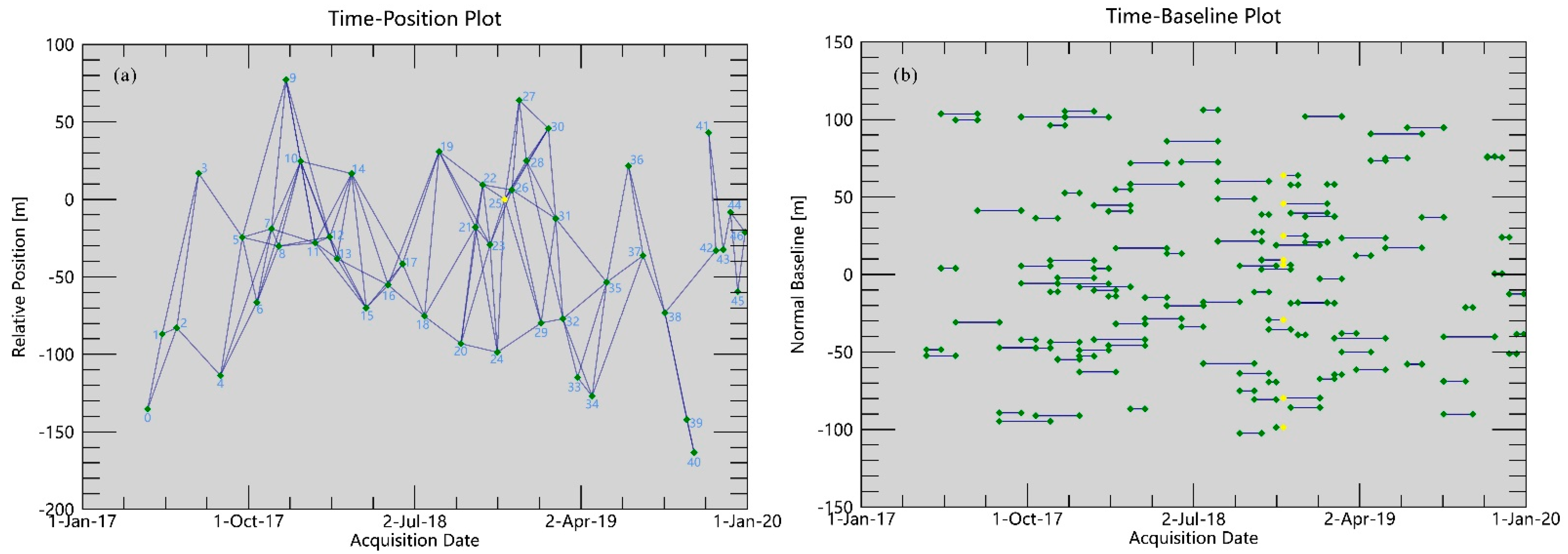
3.2.2. SBAS-InSAR
4. Results
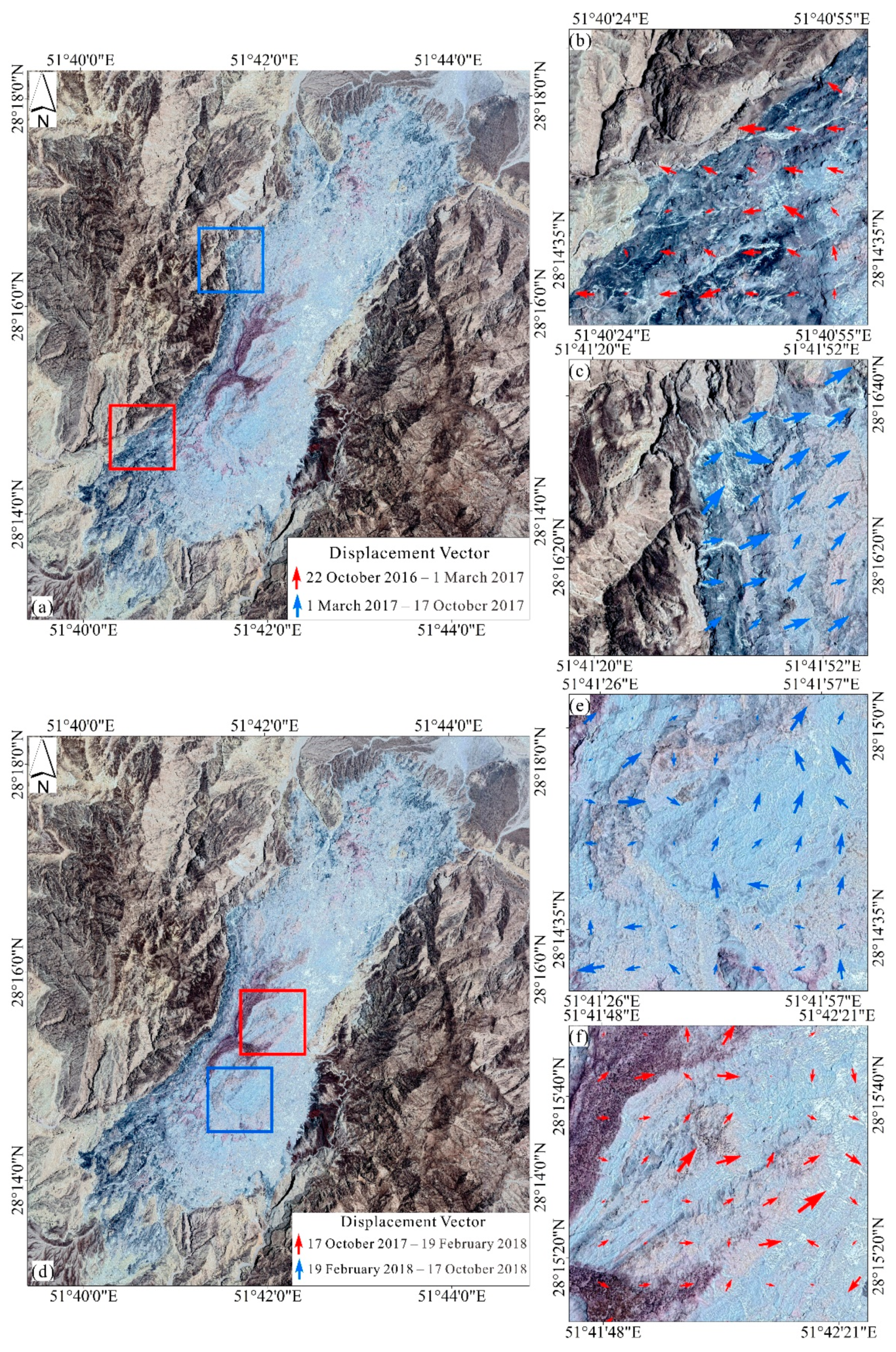
4.1. Deformation Measurements of COSI-Corr
4.2. Deformation Measurements of SBAS-InSAR
4.3. Kinematics of Kuh-e-Namak (Dashti) Namakier
5. Discussion
5.1. Relationship between Salt Kinematics and Weather Conditions
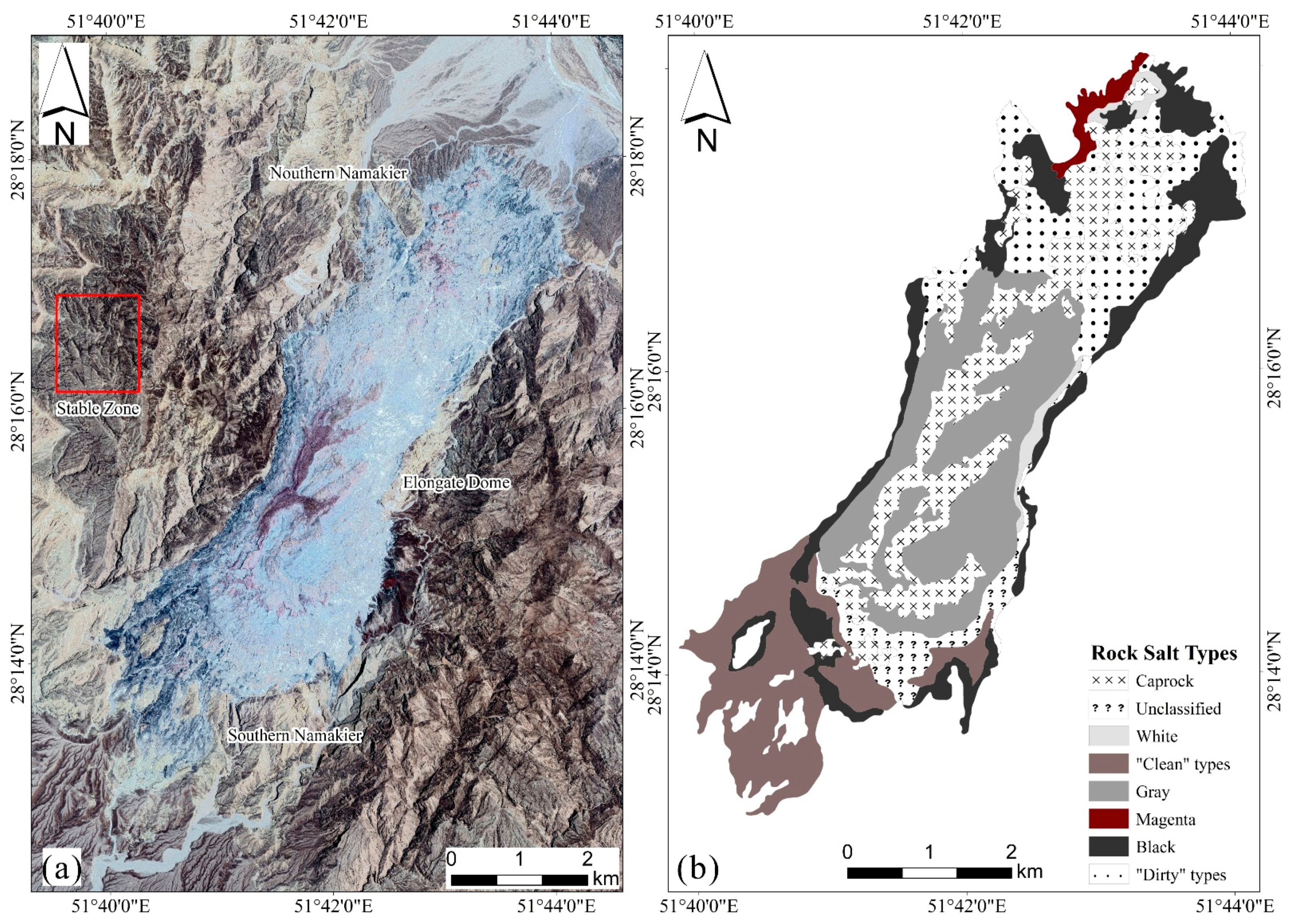
5.2. Relationship between Salt Kinematics and Rock Salt Types
5.3. Comparison of COSI-Corr and SBAS-InSAR Methods
6. Conclusions
Author Contributions
Funding
Institutional Review Board Statement
Informed Consent Statement
Data Availability Statement
Acknowledgments
Conflicts of Interest
References
- Seni, S.; Geology, B.O.E.; Jackson, M.; Bramson, R.; Burks, R.; Conti, R.; Ghazi, S.; Lovell, S.; Richter, B.; Smith, J.; et al. Sedimentary Record of Cretaceous and Tertiary Salt Movement, East. Texas Basin: Times, Rates, and Volumes of Salt Flow and Their Implications for Nuclear Waste Isolation and Petroleum Exploration; The University of Texas, Bureau of Economic Geology: Austin, TX, USA, 1984. [Google Scholar]
- Jenyon, M.K. Salt Tectonics; Elsevier Applied Science Publishers: London, UK, 1986; ISBN 1851660151. [Google Scholar]
- Thoms, R.L.; Gehle, R.M. A Brief History of Salt Cavern Use; A brief History of Salt Cavern Use (keynote paper). In Proceedings of the 8th World Salt Symposium, The Hague, The Netherlands, 7–11 May 2020; Elsevier: Amsterdam, The Netherlands, 2000. [Google Scholar]
- Talbot, C.J.; Alavi, M. The past of a future syntaxis across the Zagros. Geol. Soc. Lond. Spec. Publ. 1996, 100, 89–109. [Google Scholar] [CrossRef]
- Alsouki, M.; Riahi, M.A.; Yassaghi, A. Seismic imaging of sub-circular salt-related structures: Evidence for passive diapirism in the Straits of Hormuz, Persian Gulf. Pet. Geosci. 2011, 17, 101–107. [Google Scholar] [CrossRef]
- Talbot, C.; Aftabi, P. Geology and models of salt extrusion at Qum Kuh, central Iran. J. Geol. Soc. 2004, 161, 321–334. [Google Scholar] [CrossRef]
- Hudec, M.R.; Jackson, M.P.A. Advance of allochthonous salt sheets in passive margins and orogens. AAPG Bull. 2006, 90, 1535–1564. [Google Scholar] [CrossRef]
- Jackson, M.; Cornelius, R.R.; Craig, C.H.; Talbot, C.; Gansser, A.; Stöcklin, J. Salt diapirs of the Great Kavir, Central Iran. In GSA Memoirs; Geological Society of America: Boulder, CO, USA, 1990; Volume 177, pp. 1–150. [Google Scholar]
- Talbot, C. Fold trains in a glacier of salt in southern Iran. J. Struct. Geol. 1979, 1, 5–18. [Google Scholar] [CrossRef]
- Talbot, C.J.; Rogers, E.A. Seasonal movements in a salt glacier in Iran. Science 1980, 208, 395–397. [Google Scholar] [CrossRef] [PubMed]
- Talbot, C.J.; Jarvis, R.J. Dynamics, budget and age of an active salt extrusion. Geol. Föreningen Stockh. Förhandlingar 1983, 105, 377–378. [Google Scholar] [CrossRef]
- Závada, P.; Desbois, G.; Urai, J.L.; Schullman, K.; Rahmati, M.; Lexa, O.; Wollenberg, U.; Schulmann, K. Impact of solid second phases on deformation mechanisms of naturally deformed salt rocks (Kuh-e-Namak, Dashti, Iran) and rheological stratification of the Hormuz salt formation. J. Struct. Geol. 2015, 74, 117–144. [Google Scholar] [CrossRef]
- Talbot, C.J. Salt extrusion at Kuh-e-Jahani, Iran, from June 1994 to November 1997. Geol. Soc. Lond. Spec. Publ. 2000, 174, 93–110. [Google Scholar] [CrossRef]
- Baikpour, S.; Zulauf, G.; Dehghani, M.; Bahroudi, A. InSAR maps and time series observations of surface displacements of rock salt extruded near Garmsar, northern Iran. J. Geol. Soc. 2010, 167, 171–181. [Google Scholar] [CrossRef]
- Aftabi, P.; Roustaie, M.; Alsop, G.; Talbot, C.J. InSAR mapping and modelling of an active Iranian salt extrusion. J. Geol. Soc. 2010, 167, 155–170. [Google Scholar] [CrossRef]
- Zebker, H.A.; Goldstein, R.M. Topographic mapping from interferometric synthetic aperture radar observations. J. Geophys. Res. Solid Earth 1986, 91, 4993–4999. [Google Scholar] [CrossRef]
- Gabriel, A.K.; Goldstein, R.M.; Zebker, H.A. Mapping small elevation changes over large areas: Differential radar interferometry. J. Geophys. Res. Space Phys. 1989, 94, 9183–9191. [Google Scholar] [CrossRef]
- Ferretti, A.; Prati, C.; Rocca, F. Nonlinear subsidence rate estimation using permanent scatterers in differential SAR interferometry. IEEE Trans. Geosci. Remote Sens. 2000, 38, 2202–2212. [Google Scholar] [CrossRef] [Green Version]
- Ferretti, A.; Prati, C.; Rocca, F. Permanent scatterers in SAR interferometry. IEEE Trans. Geosci. Remote Sens. 2001, 39, 8–20. [Google Scholar] [CrossRef]
- Berardino, P.; Fornaro, G.; Lanari, R.; Sansosti, E. A new algorithm for surface deformation monitoring based on small baseline differential SAR interferograms. IEEE Trans. Geosci. Remote Sens. 2002, 40, 2375–2383. [Google Scholar] [CrossRef] [Green Version]
- Lanari, R.; Mora, O.; Manunta, M.; Mallorquí, J.J.; Berardino, P.; Sansosti, E. A small-baseline approach for investigating de-formations on full-resolution differential SAR interferograms. IEEE Trans. Geosci. Remote Sens. 2004, 42, 1377–1386. [Google Scholar] [CrossRef]
- Barnhart, W.D.; Lohman, R.B. Regional trends in active diapirism revealed by mountain range-scale InSAR time series. Geophys. Res. Lett. 2012, 39. [Google Scholar] [CrossRef]
- Abdolmaleki, N.; Motagh, M.; Bahroudi, A.; Sharifi, M.A.; Haghighi, M.H. Using Envisat InSAR time-series to investigate the surface kinematics of an active salt extrusion near Qum, Iran. J. Geodyn. 2014, 81, 56–66. [Google Scholar] [CrossRef]
- Colón, C.; Webb, A.A.G.; Lasserre, C.; Doin, M.-P.; Renard, F.; Lohman, R.; Li, J.; Baudoin, P.F. The variety of subaerial active salt deformations in the Kuqa fold-thrust belt (China) constrained by InSAR. Earth Planet. Sci. Lett. 2016, 450, 83–95. [Google Scholar] [CrossRef] [Green Version]
- Roosta, H.; Jalalifar, H.; Nasab, S.K.; Ranjbar, M. Surface deformation over the buried Nasr Abad salt diapir, Central Iran using interferometric synthetic aperture radar data. Int. J. Remote Sens. 2019, 40, 8322–8341. [Google Scholar] [CrossRef]
- Leprince, S.; Barbot, S.; Ayoub, F.; Avouac, J.-P. Automatic and precise orthorectification, coregistration, and subpixel correlation of satellite images, application to ground deformation measurements. IEEE Trans. Geosci. Remote Sens. 2007, 45, 1529–1558. [Google Scholar] [CrossRef] [Green Version]
- Heid, T.; Kääb, A. Evaluation of existing image matching methods for deriving glacier surface displacements globally from optical satellite imagery. Remote Sens. Environ. 2012, 118, 339–355. [Google Scholar] [CrossRef]
- Singh, K.K.; Singh, D.K.; Negi, H.S.; Kulkarni, A.V.; Gusain, H.S.; Ganju, A.; Raj, K.B.G. Temporal change and flow velocity estimation of Patseo Glacier, Western Himalaya, India. Curr. Sci. 2018, 114, 776–784. [Google Scholar] [CrossRef]
- Stumpf, A.; Malet, J.-P.; Allemand, P.; Ulrich, P. Surface reconstruction and landslide displacement measurements with Pléiades satellite images. ISPRS J. Photogramm. Remote Sens. 2014, 95, 1–12. [Google Scholar] [CrossRef]
- Turner, D.; Lucieer, A.; De Jong, S.M. Time series analysis of landslide dynamics using an unmanned aerial vehicle (UAV). Remote Sens. 2015, 7, 1736–1757. [Google Scholar] [CrossRef] [Green Version]
- Vermeesch, P.; Drake, N. Remotely sensed dune celerity and sand flux measurements of the world’s fastest barchans (Bodélé, Chad). Geophys. Res. Lett. 2008, 35, L24404. [Google Scholar] [CrossRef] [Green Version]
- Baird, T.; Bristow, C.S.; Vermeesch, P. Measuring sand dune migration rates with COSI-Corr and Landsat: Opportunities and challenges. Remote Sens. 2019, 11, 2423. [Google Scholar] [CrossRef] [Green Version]
- Barisin, I.; Leprince, S.; Parsons, B.; Wright, T. Surface displacements in the September 2005 Afar rifting event from satellite image matching: Asymmetric uplift and faulting. Geophys. Res. Lett. 2009, 36, 420–439. [Google Scholar] [CrossRef] [Green Version]
- Milliner, C.W.D.; Dolan, J.F.; Hollingsworth, J.; Leprince, S.; Ayoub, F.; Sammis, C.G. Quantifying near-field and off-fault deformation patterns of the 1992 Mw 7.3 Landers earthquake. Geochem. Geophys. Geosystems 2015, 16, 1577–1598. [Google Scholar] [CrossRef] [Green Version]
- Edgell, H.S. Salt tectonism in the Persian Gulf Basin. Geol. Soc. Lond. Spec. Publ. 1996, 100, 129–151. [Google Scholar] [CrossRef]
- Kent, P.E. The emergent Hormuz salt plugs of Southern Iran. J. Pet. Geol. 1979, 2, 117–144. [Google Scholar] [CrossRef]
- Mohr, M.; Warren, J.K.; Kukla, P.A.; Urai, J.L.; Irmen, A. Subsurface seismic record of salt glaciers in an extensional intracontinental setting (Late Triassic of northwestern Germany). Geology 2007, 35, 963. [Google Scholar] [CrossRef]
- Talbot, C.J.; Pohjola, V. Subaerial salt extrusions in Iran as analogues of ice sheets, streams and glaciers. Earth-Sci. Rev. 2009, 97, 155–183. [Google Scholar] [CrossRef]
- Talbot, C.J. Extrusions of Hormuz salt in Iran. Geol. Soc. Lond. Spec. Publ. 1998, 143, 315–334. [Google Scholar] [CrossRef]
- Ahrens, T.J. Rock Physics & Phase Relations: A Handbook of Physical Constants; AGU Reference Shelf 3; American Geophysical Union: Washington, DC, USA, 1995; ISBN 0875908535. [Google Scholar]
- Gascon, F.; Bouzinac, C.; Thépaut, O.; Jung, M.; Francesconi, B.; Louis, J.; Lonjou, V.; Lafrance, B.; Massera, S.; Gaudel-Vacaresse, A.; et al. Copernicus sentinel-2A calibration and products validation status. Remote Sens. 2017, 9, 584. [Google Scholar] [CrossRef] [Green Version]
- Scherler, D.; Leprince, S.; Strecker, M. Glacier-surface velocities in alpine terrain from optical satellite imagery—Accuracy improvement and quality assessment. Remote Sens. Environ. 2008, 112, 3806–3819. [Google Scholar] [CrossRef]
- Ali, E.; Xu, W.; Ding, X. Improved optical image matching time series inversion approach for monitoring dune migration in North Sinai Sand Sea: Algorithm procedure, application, and validation. ISPRS J. Photogramm. Remote Sens. 2020, 164, 106–124. [Google Scholar] [CrossRef]
- Yang, W.; Wang, Y.; Wang, Y.; Ma, C.; Ma, Y. Retrospective deformation of the Baige landslide using optical remote sensing images. Landslides 2019, 17, 659–668. [Google Scholar] [CrossRef]
- Zhou, L.; Guo, J.; Hu, J.; Li, J.; Xu, Y.; Pan, Y.; Shi, M. Wuhan surface subsidence analysis in 2015–2016 based on sentinel-1a data by SBAS-inSAR. Remote Sens. 2017, 9, 982. [Google Scholar] [CrossRef] [Green Version]
- Hooper, A. A multi-temporal InSAR method incorporating both persistent scatterer and small baseline approaches. Geophys. Res. Lett. 2008, 35. [Google Scholar] [CrossRef] [Green Version]
- Goldstein, R.M.; Werner, C.L. Radar interferogram filtering for geophysical applications. Geophys. Res. Lett. 1998, 25, 4035–4038. [Google Scholar] [CrossRef] [Green Version]
- Costantini, M. A novel phase unwrapping method based on network programming. IEEE Trans. Geosci. Remote Sens. 1998, 36, 813–821. [Google Scholar] [CrossRef]
- Gaber, A.; Darwish, N.; Koch, M. Minimizing the residual topography effect on interferograms to improve DInSAR results: Estimating land subsidence in Port-Said City, Egypt. Remote Sens. 2017, 9, 752. [Google Scholar] [CrossRef] [Green Version]
- Pepe, A.; Berardino, P.; Bonano, M.; Euillades, L.D.; Lanari, R.; Sansosti, E. SBAS-based satellite orbit correction for the generation of DInSAR time-series: Application to RADARSAT-1 Data. IEEE Trans. Geosci. Remote Sens. 2011, 49, 5150–5165. [Google Scholar] [CrossRef]
- Kuo, Y.; Yang, T.; Huang, G.-W. The use of grey relational analysis in solving multiple attribute decision-making problems. Comput. Ind. Eng. 2008, 55, 80–93. [Google Scholar] [CrossRef]


| Sensor | Acquisition Dates (YYMMDD) | Orbit Number | Cloud Cover (Percentage) | Sun Zenith Angle (Degree) | Sun Azimuth Angle (Degree) |
|---|---|---|---|---|---|
| S2A_MSIL1C | 22 October 2016 | 106 | 0.007 | 41.947 | 159.039 |
| S2A_MSIL1C | 31 December 2016 | 106 | 0.000 | 54.580 | 158.671 |
| S2A_MSIL1C | 1 March 2017 | 106 | 0.153 | 41.277 | 147.256 |
| S2A_MSIL1C | 17 October 2017 | 106 | 0.311 | 40.242 | 157.793 |
| S2B_MSIL1C | 31 December 2017 | 106 | 4.257 | 54.594 | 158.692 |
| S2B_MSIL1C | 19 February 2018 | 106 | 0.357 | 44.797 | 149.363 |
| S2B_MSIL1C | 17 October 2018 | 106 | 1.278 | 40.166 | 157.714 |
| S2B_MSIL1C | 24 February 2019 | 106 | 0.049 | 43.189 | 148.427 |
| S2B_MSIL1C | 22 October 2019 | 106 | 0.012 | 41.703 | 158.914 |
| S2A_MSIL1C | 26 December 2019 | 106 | 0.370 | 54.656 | 159.550 |
| Data | Parameters | Description |
|---|---|---|
| Sentinel-1A | Type | SLC (Single Look Complex) |
| Image Mode | IW (Interferometric Wide) | |
| Band | C | |
| Track number | 28 | |
| Polarization | VV (Vertical Polarization) | |
| Range Resolution (m) | 5 | |
| Azimuth Resolution (m) | 20 | |
| SRTM | Resolution (m) | 30 |
| Pre-Image (YYYYMMDD) | Post-Image (YYYYMMDD) | Sun Zenith Angle Differences (Degrees) | East/West Displacement (Meters) | North/South DISPLACEMENT (Meters) | SNR | |||
|---|---|---|---|---|---|---|---|---|
| Mean | Standard Deviation | Mean | Standard Deviation | Mean | Standard Deviation | |||
| 22 October 2016 | 1 March 2017 | 0.670 | −1.417 | 0.393 | 1.411 | 0.350 | 0.9959 | 0.0015 |
| 1 March 2017 | 17 October 2017 | 1.035 | 1.471 | 0.369 | 1.191 | 0.336 | 0.9957 | 0.0015 |
| 17 October 2017 | 19 February 2018 | 4.555 | −2.301 | 0.468 | −2.874 | 0.373 | 0.9948 | 0.0017 |
| 19 February 2018 | 17 October 2018 | 4.631 | −3.814 | 0.434 | 0.389 | 0.301 | 0.9950 | 0.0018 |
| 17 October 2018 | 24 February 2019 | 3.023 | 3.602 | 0.421 | −1.404 | 0.323 | 0.9947 | 0.0021 |
| 24 February 2019 | 22 October 2019 | 1.486 | −1.687 | 0.456 | 0.268 | 0.265 | 0.9955 | 0.0016 |
| 31 December 2016 | 31 December 2017 | 0.014 | −0.149 | 0.256 | −0.580 | 0.174 | 0.9977 | 0.0008 |
| 31 December 2017 | 26 December 2019 | 0.076 | −2.279 | 0.187 | 2.486 | 0.135 | 0.9978 | 0.0007 |
| Correlation Pair (YYYYMMDD) | Accumulated Precipitation (mm) | Average Temperature (°C) | Displacement (m) | Velocity (m/d) |
|---|---|---|---|---|
| 22 October 2016–1 March 2017 | 377.190 | 21.34 | 21.03 | 0.162 |
| 1 March 2017–17 October 2017 | 55.626 | 31.94 | 19.71 | 0.086 |
| 17 October 2017–19 February 2018 | 113.538 | 22.13 | 14.49 | 0.116 |
| 19 February 2018–17 October 2018 | 51.308 | 31.26 | 19.40 | 0.081 |
| 17 October 2018–24 February 2019 | 159.004 | 21.69 | 20.00 | 0.154 |
| 24 February 2019–22 October 2019 | 66.294 | 30.91 | 18.29 | 0.076 |
| 31 December 2016–31 December 2017 | 471.678 | 28.04 | 19.89 | 0.054 |
| 31 December 2016–26 December 2019 | 887.730 | 27.97 | 19.38 | 0.018 |
| Correlation Pair (YYYYMMDD) | Maximum Displacement (m) | |||||
|---|---|---|---|---|---|---|
| Black | Magenta | White | Gary | “Clean” | “Dirty” | |
| 22 October 2016–1 March 2017 | 21.03 | 4.00 | 3.44 | 3.46 | 3.62 | 19.78 |
| 1 March 2017–17 October 2017 | 11.00 | 4.77 | 3.23 | 19.71 | 3.84 | 19.19 |
| 17 October 2017–19 February 2018 | 14.49 | 3.52 | 4.81 | 4.20 | 2.86 | 5.99 |
| 19 February 2018–17 October 2018 | 17.80 | 5.09 | 4.14 | 4.32 | 7.34 | 5.62 |
| 17 October 2018–24 February 2019 | 17.88 | 4.91 | 3.48 | 20.01 | 6.92 | 5.58 |
| 24 February 2019 –22 October 2019 | 18.29 | 4.48 | 2.54 | 4.10 | 2.97 | 5.01 |
| 31 December 2016–31 December 2017 | 3.34 | 2.11 | 2.26 | 4.36 | 3.95 | 19.89 |
| 31 December 2016–26 December 2019 | 19.38 | 3.31 | 17.99 | 4.31 | 4.07 | 19.10 |
| Number of Points | Location | Average Grey Relational Degree between Average Temperature and Displacement | Average Grey Relational Degree between Accumulated Precipitation and Displacement |
|---|---|---|---|
| 2000 | Flank | 0.6026 | 0.6932 |
| 2000 | Dome | 0.6023 | 0.7030 |
| Rock Salt Types | Average Grey Relational Degree | |
|---|---|---|
| Precipitation | Temperature | |
| Black | 0.6756 | 0.5935 |
| Magenta | 0.6789 | 0.5652 |
| White | 0.6732 | 0.5725 |
| Gray | 0.7153 | 0.6078 |
| “Clean” | 0.6794 | 0.5831 |
| “Dirty” | 0.6957 | 0.5976 |
Publisher’s Note: MDPI stays neutral with regard to jurisdictional claims in published maps and institutional affiliations. |
© 2021 by the authors. Licensee MDPI, Basel, Switzerland. This article is an open access article distributed under the terms and conditions of the Creative Commons Attribution (CC BY) license (http://creativecommons.org/licenses/by/4.0/).
Share and Cite
Zhang, S.; Jiang, Q.; Shi, C.; Xu, X.; Gong, Y.; Xi, J.; Liu, W.; Liu, B. Application of Sentinel-1 and-2 Images in Measuring the Deformation of Kuh-e-Namak (Dashti) Namakier, Iran. Remote Sens. 2021, 13, 785. https://doi.org/10.3390/rs13040785
Zhang S, Jiang Q, Shi C, Xu X, Gong Y, Xi J, Liu W, Liu B. Application of Sentinel-1 and-2 Images in Measuring the Deformation of Kuh-e-Namak (Dashti) Namakier, Iran. Remote Sensing. 2021; 13(4):785. https://doi.org/10.3390/rs13040785
Chicago/Turabian StyleZhang, Sen, Qigang Jiang, Chao Shi, Xitong Xu, Yundi Gong, Jing Xi, Wenxuan Liu, and Bin Liu. 2021. "Application of Sentinel-1 and-2 Images in Measuring the Deformation of Kuh-e-Namak (Dashti) Namakier, Iran" Remote Sensing 13, no. 4: 785. https://doi.org/10.3390/rs13040785