
Remote Sensing of Atmospheric Hydrogen Fluoride (HF) over Hefei, China with Ground-Based High-Resolution Fourier Transform Infrared (FTIR) Spectrometry

 ,
,
Abstract
:
1. Introduction
2. Materials and Methods
2.1. Site Description and FTIR Instrumentation
2.2. Retrieval Strategy for NIR Spectra Suite
2.3. Retrieval Strategy for MIR Spectra Suite
2.4. Regression Model for Seasonality and Interannual Trend
2.5. Strategy for Comparing the NIR and MIR Retrievals
2.6. Data Filter Criteria
3. Results
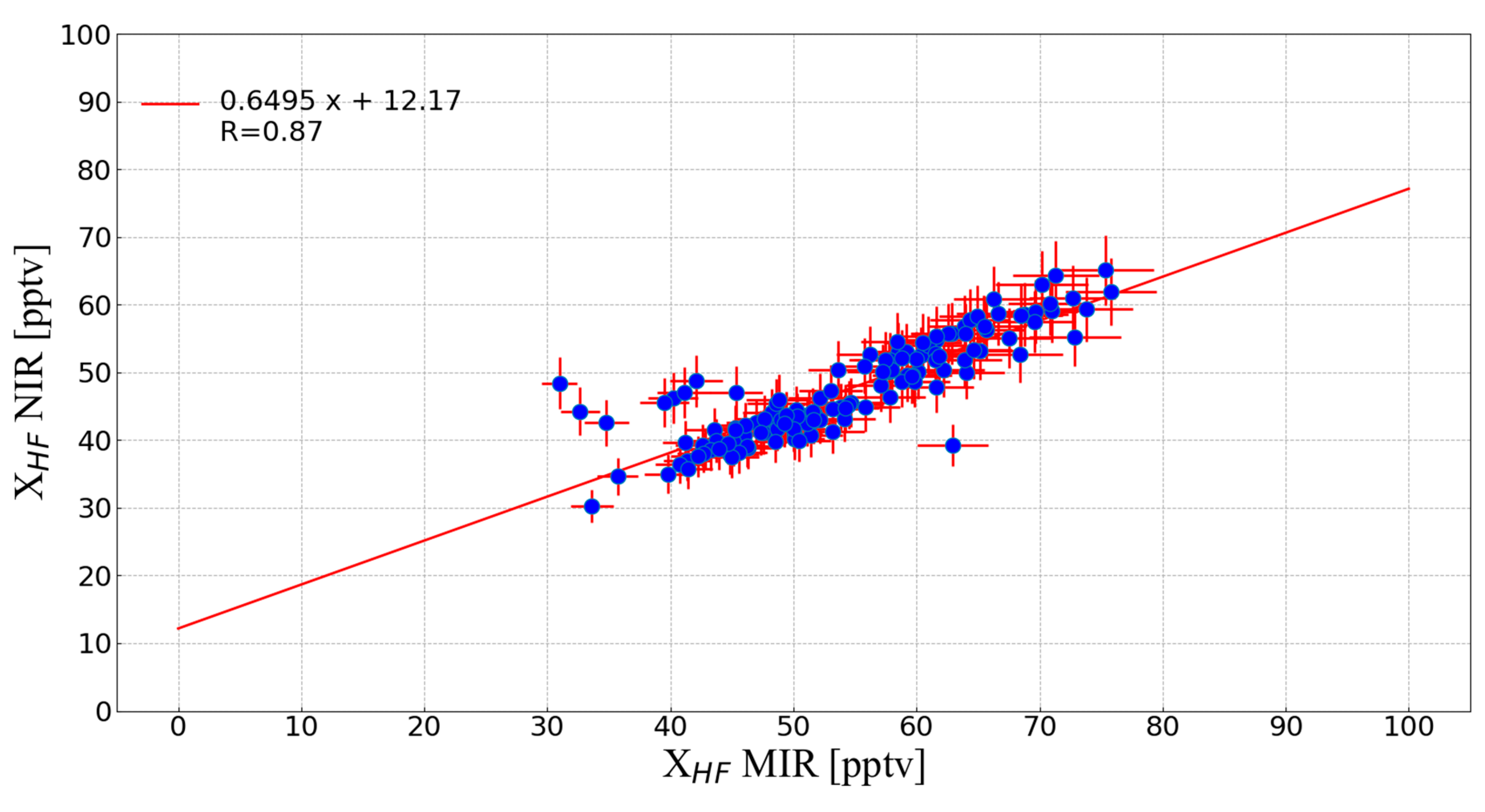
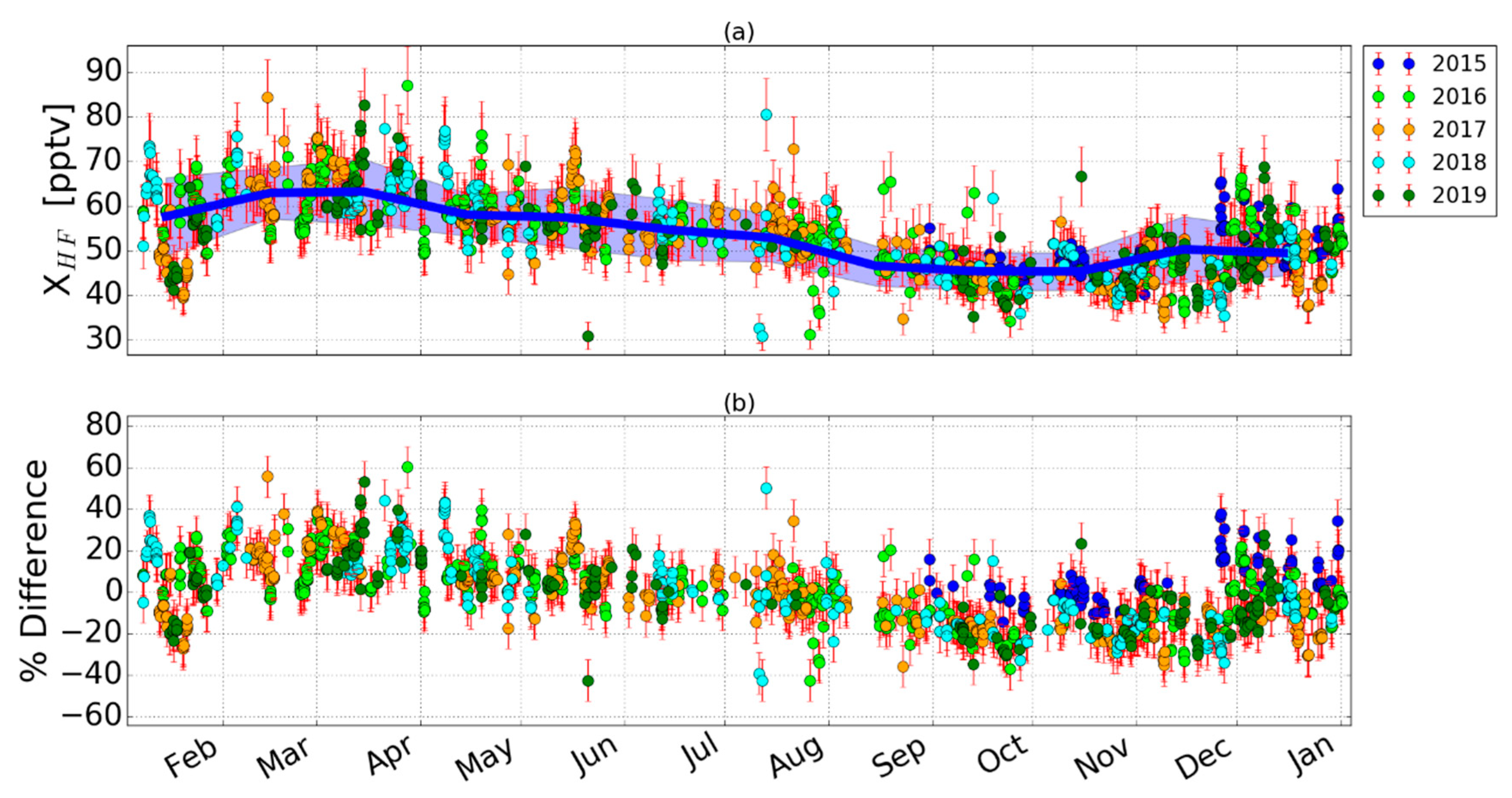
3.1. Comparison between NIR and MIR Retrievals
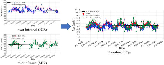
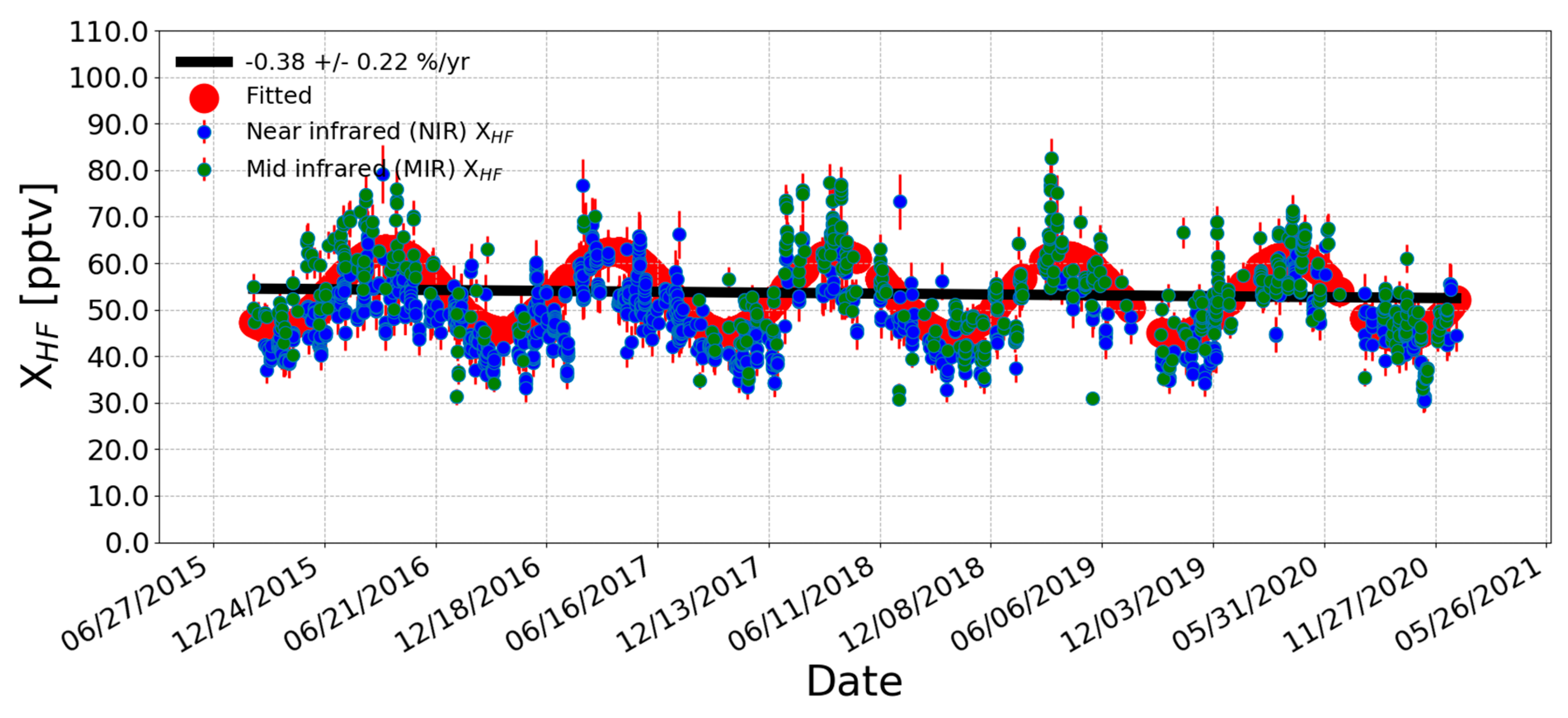
3.2. Seasonal and Interannual Variabilities
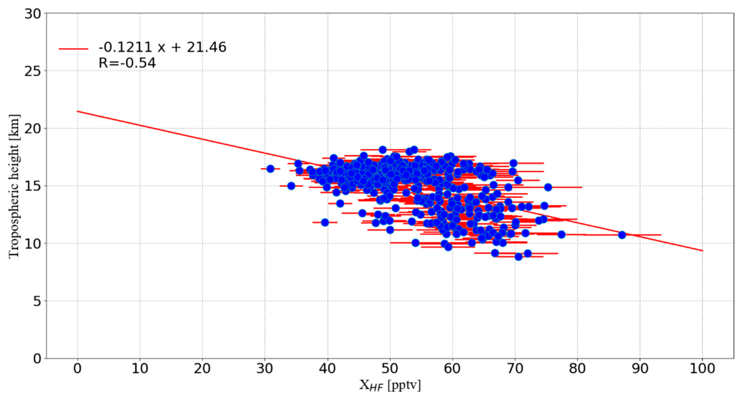
4. Discussion
5. Conclusions
Author Contributions
Funding
Data Availability Statement
Acknowledgments
Conflicts of Interest
References
- Mahieu, E.; Duchatelet, P.; Demoulin, P.; Walker, K.A.; Dupuy, E.; Froidevaux, L.; Randall, C.; Catoire, V.; Strong, K.; Boone, C.D.; et al. Validation of ACE-FTS v2.2 measurements of HCl, HF, CCl3F and CCl2F2 using space-, balloon- and ground-based instrument observations. Atmos. Chem. Phys. 2008, 8, 6199–6221. [Google Scholar] [CrossRef] [Green Version]
- Steffen, J.; Bernath, P.F.; Boone, C.D. Trends in halogen-containing molecules measured by the Atmospheric Chemistry Experiment (ACE) satellite. J. Quant. Spectrosc. Radiat. Transf. 2019, 238, 106619. [Google Scholar] [CrossRef]
- Tegtmeier, S.; Hegglin, M.I.; Anderson, J.; Funke, B.; Walker, K.A. The SPARC Data Initiative: Comparisons of CFC-11, CFC-12, HF and SF6 climatologies from international satellite limb sounders. Earth Syst. Sci. Data 2016, 8, 61–78. [Google Scholar] [CrossRef] [Green Version]
- Brown, A.T.; Chipperfield, M.P.; Richards, N.A.D.; Boone, C.; Bernath, P.F. Global stratospheric fluorine inventory for 2004-2009 from Atmospheric Chemistry Experiment Fourier Transform Spectrometer (ACE-FTS) measurements and SLIMCAT model simulations. Atmos. Chem. Phys. 2014, 14, 267–282. [Google Scholar] [CrossRef] [Green Version]
- Tressaud, A. Fluorine and the Environment: Atmospheric Chemistry, Emissions & Lithosphere; Advances in Fluorine Science; Elsevier Science: Amsterdam, The Netherlands, 2006. [Google Scholar]
- Duchatelet, P.; Demoulin, P.; Hase, F.; Ruhnke, R.; Feng, W.; Chipperfield, M.P.; Bernath, P.F.; Boone, C.D.; Walker, K.A.; Mahieu, E. Hydrogen fluoride total and partial column time series above the Jungfraujoch from long-term FTIR measurements: Impact of the line-shape model, characterization of the error budget and seasonal cycle, and comparison with satellite and model data. J. Geophys. Res. Atmos. 2010, 115. [Google Scholar] [CrossRef] [Green Version]
- Harrison, J.J.; Chipperfield, M.P.; Boone, C.D.; Dhomse, S.S.; Russell, J. Satellite observations of stratospheric hydrogen fluoride and comparisons with SLIMCAT calculations. Atmos. Chem. Phys. 2015, 15, 34361–34405. [Google Scholar]
- Rinsland, C.P.; Boone, C.; Nassar, R.; Walker, K.; Bernath, P.; Mahieu, E.; Zander, R.; McConnell, J.C.; Chiou, L. Trends of HF, HCl, CCl2F2, CCl3F, CHClF2 (HCFC-22), and SF6 in the lower stratosphere from Atmospheric Chemistry Experiment (ACE) and Atmospheric Trace Molecule Spectroscopy (ATMOS) measurements near 30°N latitude. Geophys. Res. Lett. 2005, 32. [Google Scholar] [CrossRef] [Green Version]
- Mikuteit, S. Trendbestimmung Stratosphärischer Spurengase Mit Hilfe Bodengebundener FTIR-Messungen. Ph.D. Thesis, Forschungszentrum Karlsruhe, Karlsruhe, Germany, 2008. [Google Scholar]
- Kohlhepp, R.; Barthlott, S.; Blumenstock, T.; Hase, F.; Kaiser, I.; Raffalski, U.; Ruhnke, R. Trends of HCl, ClONO2, and HF column abundances from ground-based FTIR measurements in Kiruna (Sweden) in comparison with KASIMA model calculations. Atmos. Chem. Phys. 2011, 11, 4669–4677. [Google Scholar] [CrossRef] [Green Version]
- Messerschmidt, J.; Macatangay, R.; Notholt, J.; Petri, C.; Warneke, T.; Weinzierl, C. Side by side measurements of CO2 by ground-based Fourier transform spectrometry (FTS). Tellus B 2010, 62, 749–758. [Google Scholar] [CrossRef] [Green Version]
- Washenfelder, R.A.; Toon, G.C.; Blavier, J.F.; Yang, Z.; Allen, N.T.; Wennberg, P.O.; Vay, S.A.; Matross, D.M.; Daube, B.C. Carbon dioxide column abundances at the Wisconsin Tall Tower site. J. Geophys. Res. Atmos. 2006, 111, D22305. [Google Scholar] [CrossRef] [Green Version]
- Wunch, D.; Toon, G.C.; Blavier, J.F.L.; Washenfelder, R.A.; Notholt, J.; Connor, B.J.; Griffith, D.W.T.; Sherlock, V.; Wennberg, P.O. The Total Carbon Column Observing Network. Philos. Trans. R. Soc. A 2011, 369, 2087–2112. [Google Scholar] [CrossRef] [PubMed] [Green Version]
- Wunch, D.; Toon, G.C.; Wennberg, P.O.; Wofsy, S.C.; Stephens, B.B.; Fischer, M.L.; Uchino, O.; Abshire, J.B.; Bernath, P.; Biraud, S.C.; et al. Calibration of the Total Carbon Column Observing Network using aircraft profile data. Atmos. Meas. Tech. 2010, 3, 1351–1362. [Google Scholar] [CrossRef] [Green Version]
- Angelbratt, J.; Mellqvist, J.; Simpson, D.; Jonson, J.E.; Blumenstock, T.; Borsdorff, T.; Duchatelet, P.; Forster, F.; Hase, F.; Mahieu, E.; et al. Carbon monoxide (CO) and ethane (C2H6) trends from ground-based solar FTIR measurements at six European stations, comparison and sensitivity analysis with the EMEP model. Atmos. Chem. Phys. 2011, 11, 9253–9269. [Google Scholar] [CrossRef] [Green Version]
- Zhou, M.; Langerock, B.; Vigouroux, C.; Sha, M.K.; Hermans, C.; Metzger, J.M.; Chen, H.; Ramonet, M.; Kivi, R.; Heikkinen, P.; et al. TCCON and NDACC XCO measurements: Difference, discussion and application. Atmos. Meas. Tech. 2019, 12, 5979–5995. [Google Scholar] [CrossRef] [Green Version]
- Zhou, M.; Langerock, B.; Wells, K.C.; Millet, D.B.; Vigouroux, C.; Sha, M.K.; Hermans, C.; Metzger, J.M.; Kivi, R.; Heikkinen, P.; et al. An intercomparison of total column-averaged nitrous oxide between ground-based FTIR TCCON and NDACC measurements at seven sites and comparisons with the GEOS-Chem model. Atmos. Meas. Tech. 2019, 12, 1393–1408. [Google Scholar] [CrossRef] [Green Version]
- Sun, Y.W.; Liu, C.; Palm, M.; Vigouroux, C.; Notholt, J.; Hui, Q.H.; Jones, N.; Wang, W.; Su, W.J.; Zhang, W.Q.; et al. Ozone seasonal evolution and photochemical production regime in the polluted troposphere in eastern China derived from high-resolution Fourier transform spectrometry (FTS) observations. Atmos. Chem. Phys. 2018, 18, 14569–14583. [Google Scholar] [CrossRef] [Green Version]
- Sun, Y.; Yin, H.; Liu, C.; Zhang, L.; Cheng, Y.; Palm, M.; Notholt, J.; Lu, X.; Vigouroux, C.; Zheng, B.; et al. Mapping the drivers of formaldehyde (HCHO) variability from 2015–2019 over eastern China: Insights from FTIR observation and GEOS-Chem model simulation. Atmos. Chem. Phys. Discuss. 2020, 2020, 1–24. [Google Scholar] [CrossRef]
- Sun, Y.W.; Liu, C.; Zhang, L.; Palm, M.; Notholt, J.; Hao, Y.; Vigouroux, C.; Lutsch, E.; Wang, W.; Shan, C.G.; et al. Fourier transform infrared time series of tropospheric HCN in eastern China: Seasonality, interannual variability, and source attribution. Atmos. Chem. Phys. 2020, 20, 5437–5456. [Google Scholar] [CrossRef]
- Tian, Y.; Sun, Y.W.; Liu, C.; Wang, W.; Shan, C.G.; Xu, X.W.; Hu, Q.H. Characterisation of methane variability and trends from near-infrared solar spectra over Hefei, China. Atmos. Environ. 2018, 173, 198–209. [Google Scholar] [CrossRef]
- Wang, W.; Tian, Y.; Liu, C.; Sun, Y.W.; Liu, W.Q.; Xie, P.H.; Liu, J.G.; Xu, J.; Morino, I.; Velazco, V.A.; et al. Investigating the performance of a greenhouse gas observatory in Hefei, China. Atmos. Meas. Tech. 2017, 10, 2627–2643. [Google Scholar] [CrossRef] [Green Version]
- Yin, H.; Sun, Y.W.; Liu, C.; Lu, X.; Smale, D.; Blumenstock, T.; Nagahama, T.; Wang, W.; Tian, Y.; Hu, Q.H.; et al. Ground-based FTIR observation of hydrogen chloride (HCl) over Hefei, China, and comparisons with GEOS-Chem model data and other ground-based FTIR stations data. Opt. Express 2020, 28, 8041–8055. [Google Scholar] [CrossRef] [PubMed]
- Yin, H.; Sun, Y.W.; Liu, C.; Zhang, L.; Lu, X.; Wang, W.; Shan, C.G.; Hu, Q.H.; Tian, Y.; Zhang, C.X.; et al. FTIR time series of stratospheric NO2 over Hefei, China, and comparisons with OMI and GEOS-Chem model data. Opt. Express 2019, 27, A1225–A1240. [Google Scholar] [CrossRef] [PubMed]
- Shan, C.G.; Wang, W.; Liu, C.; Sun, Y.W.; Hu, Q.H.; Xu, X.W.; Tian, Y.; Zhang, H.F.; Morino, I.; Griffit, D.W.T.; et al. Regional CO emission estimated from ground-based remote sensing at Hefei site, China. Atmos. Res. 2019, 222, 25–35. [Google Scholar] [CrossRef] [Green Version]
- Sun, Y.W.; Palm, M.; Liu, C.; Hase, F.; Griffith, D.; Weinzierl, C.; Petri, C.; Wang, W.; Notholt, J. The influence of instrumental line shape degradation on NDACC gas retrievals: Total column and profile. Atmos. Meas. Tech. 2018, 11, 2879–2896. [Google Scholar] [CrossRef] [Green Version]
- Wunch, D.; Toon, G.C.; Sherlock, V.; Deutscher, N.M.; Liu, X.; Feist, D.G.; Wennberg, P.O. The Total Carbon Column Observing Network’s GGG2014 Data Version. CaltechDATA 2015. [Google Scholar] [CrossRef]
- Kalnay, E.; Kanamitsu, M.; Kistler, R.; Collins, W.; Deaven, D.; Gandin, L.; Iredell, M.; Saha, S.; White, G.; Woollen, J.; et al. The NCEP/NCAR 40-year reanalysis project. Am. Meteorol. Soc. 1996, 77, 437–471. [Google Scholar] [CrossRef] [Green Version]
- Hill, C.; Gordon, I.E.; Rothman, L.S.; Tennyson, J. A new relational database structure and online interface for the HITRAN database. J. Quant. Spectrosc. Radiat. Transf. 2013, 130, 51–61. [Google Scholar] [CrossRef]
- Rothman, L.S.; Gordon, I.E.; Barbe, A.; Benner, D.C.; Bernath, P.F.; Birk, M.; Boudon, V.; Brown, L.R.; Campargue, A.; Champion, J.P.; et al. The HITRAN 2008 molecular spectroscopic database. J. Quant. Spectrosc. Radiat. Transf. 2009, 110, 533–572. [Google Scholar] [CrossRef] [Green Version]
- Hase, F. Improved instrumental line shape monitoring for the ground-based, high-resolution FTIR spectrometers of the Network for the Detection of Atmospheric Composition Change. Atmos. Meas. Tech. 2012, 5, 603–610. [Google Scholar] [CrossRef] [Green Version]
- Hase, F.; Blumenstock, T.; Paton-Walsh, C. Analysis of the instrumental line shape of high-resolution Fourier transform IR spectrometers with gas cell measurements and new retrieval software. Appl. Opt. 1999, 38, 3417–3422. [Google Scholar] [CrossRef]
- Rodgers, C. Inverse Methods for Atmospheric Sounding—Theory and Practice; World Scientific: Singapore, 2000; Volume 2. [Google Scholar] [CrossRef]
- Rodgers, C.D.; Connor, B.J. Intercomparison of remote sounding instruments. J. Geophys. Res. Atmos. 2003, 108. [Google Scholar] [CrossRef] [Green Version]
- Gardiner, T.; Forbes, A.; de Maziere, M.; Vigouroux, C.; Mahieu, E.; Demoulin, P.; Velazco, V.; Notholt, J.; Blumenstock, T.; Hase, F.; et al. Trend analysis of greenhouse gases over Europe measured by a network of ground-based remote FTIR instruments. Atmos. Chem. Phys. 2008, 8, 6719–6727. [Google Scholar] [CrossRef] [Green Version]
- Santer, B.D.; Thorne, P.W.; Haimberger, L.; Taylor, K.E.; Wigley, T.M.L.; Lanzante, J.R.; Solomon, S.; Free, M.; Gleckler, P.J.; Jones, P.D.; et al. Consistency of modelled and observed temperature trends in the tropical troposphere. Int. J. Clim. 2008, 28, 1703–1722. [Google Scholar] [CrossRef]
- Kohlhepp, R.; Ruhnke, R.; Chipperfield, M.P.; De Maziere, M.; Notholt, J.; Barthlott, S.; Batchelor, R.L.; Blatherwick, R.D.; Blumenstock, T.; Coffey, M.T.; et al. Observed and simulated time evolution of HCl, ClONO2, and HF total column abundances. Atmos. Chem. Phys. 2012, 12, 3527–3556. [Google Scholar] [CrossRef] [Green Version]
- Vigouroux, C.; De Mazière, M.; Demoulin, P.; Servais, C.; Hase, F.; Blumenstock, T.; Kramer, I.; Schneider, M.; Mellqvist, J.; Strandberg, A.; et al. Evaluation of tropospheric and stratospheric ozone trends over Western Europe from ground-based FTIR network observations. Atmos. Chem. Phys. 2008, 8, 6865–6886. [Google Scholar] [CrossRef] [Green Version]


| Gases | HF | O2 |
|---|---|---|
| Retrieval code | GGG2014 | GGG2014 |
| Spectroscopy | HITRAN2008 | HITRAN2008 |
| Pressure, Temperature profiles | NCEP | NCEP |
| A priori profiles for all gases | GGG2014 code | GGG2014 code |
| MW for profile retrievals (cm−1) | 4038.79–4039.11 | 7765–8005 |
| Window Width (cm−1) | 0.32 | 240 |
| Retrieved interfering gases | H2O | CO2, H2O, HF |
| Gases | HF | |
|---|---|---|
| Retrieval code | SFIT4 v 0.9.4.4 | |
| Spectroscopy | HITRAN2008 | |
| P, T profiles | NCEP | |
| A priori profiles for all gases except H2O | WACCM v6 | |
| MW for profile retrievals (cm−1) | 4109.4-4110.20 | |
| Window Width (cm−1) | 0.8 | |
| Retrieved interfering gases | CH4, HDO and H2O | |
| De-weighting SNR | None | |
| Regularization | Sa | WACCM Std |
| Sε | Real SNR | |
| ILS | LINEFIT145 | |
| Gases | Kb | HF |
|---|---|---|
| Temperature uncertainty | SD of NCEP | 0.41% |
| Retrieval parameters uncertainty | * | <0.01% |
| Interfering species uncertainty | * | <0.01% |
| Measurement error | * | 0.29% |
| Smoothing uncertainty | * | 0.15% |
| Total random error | / | 0.52% |
| Background curvature uncertainty | 0.1% | 0.03% |
| Optical path difference uncertainty | 0.1% | <0.01% |
| Field of view uncertainty | 0.1% | <0.01% |
| Solar line strength uncertainty | 0.1% | <0.01% |
| Solar line shift uncertainty | 0.1% | <0.01% |
| Phase uncertainty | 0.1% | <0.01% |
| Line temperature broadening uncertainty | 5% | 0.01% |
| Line pressure broadening uncertainty | 5% | 1.22% |
| Line intensity uncertainty | 5% | 5.00% |
| Total systematic error | / | 5.15% |
| Total error | / | 5.18% |
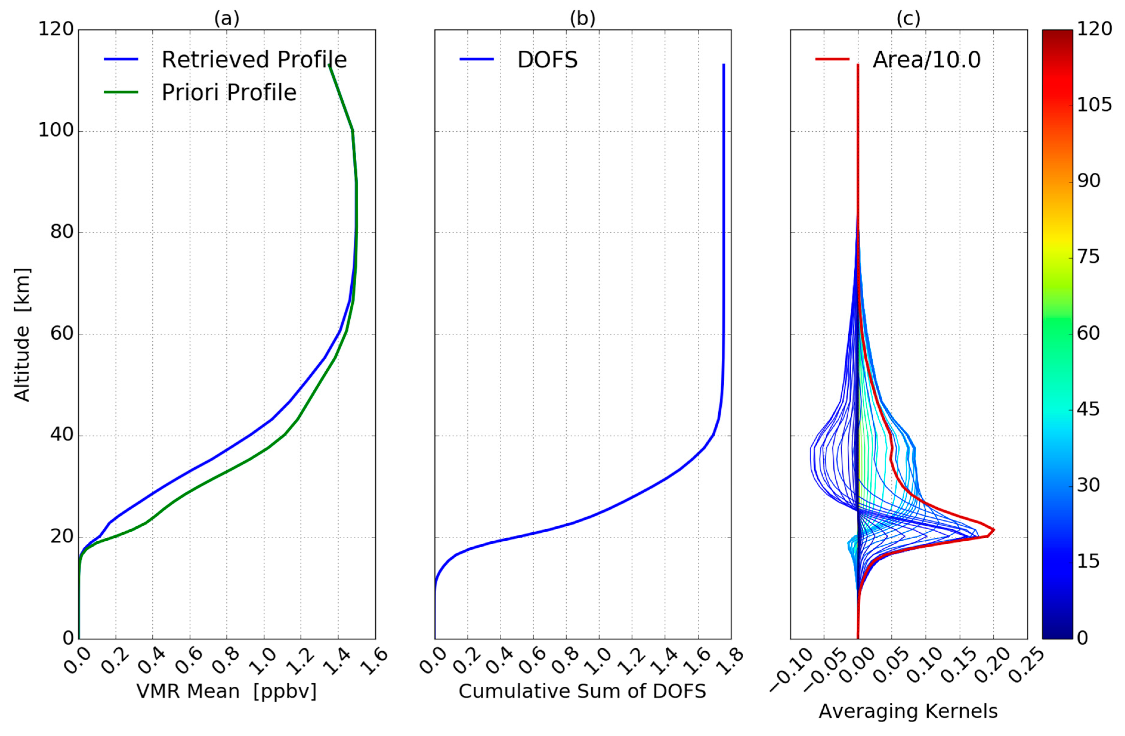
| DOFS (-) | / | 1.76 |
Publisher’s Note: MDPI stays neutral with regard to jurisdictional claims in published maps and institutional affiliations. |
© 2021 by the authors. Licensee MDPI, Basel, Switzerland. This article is an open access article distributed under the terms and conditions of the Creative Commons Attribution (CC BY) license (http://creativecommons.org/licenses/by/4.0/).
Share and Cite
Yin, H.; Sun, Y.; Liu, C.; Wang, W.; Shan, C.; Zha, L. Remote Sensing of Atmospheric Hydrogen Fluoride (HF) over Hefei, China with Ground-Based High-Resolution Fourier Transform Infrared (FTIR) Spectrometry. Remote Sens. 2021, 13, 791. https://doi.org/10.3390/rs13040791
Yin H, Sun Y, Liu C, Wang W, Shan C, Zha L. Remote Sensing of Atmospheric Hydrogen Fluoride (HF) over Hefei, China with Ground-Based High-Resolution Fourier Transform Infrared (FTIR) Spectrometry. Remote Sensing. 2021; 13(4):791. https://doi.org/10.3390/rs13040791
Chicago/Turabian StyleYin, Hao, Youwen Sun, Cheng Liu, Wei Wang, Changgong Shan, and Lingling Zha. 2021. "Remote Sensing of Atmospheric Hydrogen Fluoride (HF) over Hefei, China with Ground-Based High-Resolution Fourier Transform Infrared (FTIR) Spectrometry" Remote Sensing 13, no. 4: 791. https://doi.org/10.3390/rs13040791