Abstract
Successfully applied in the carbon research area, sun-induced chlorophyll fluorescence (SIF) has raised the interest of researchers from the water research domain. However, current works focused on the empirical relationship between SIF and plant transpiration (T), while the mechanistic linkage between them has not been fully explored. Two mechanism methods were developed to estimate T via SIF, namely the water-use efficiency (WUE) method and conductance method based on the carbon–water coupling framework. The T estimated by these two methods was compared with T partitioned from eddy covariance instrument measured evapotranspiration at four different sites. Both methods showed good performance at the hourly (R2 = 0.57 for the WUE method and 0.67 for the conductance method) and daily scales (R2 = 0.67 for the WUE method and 0.78 for the conductance method). The developed mechanism methods provide theoretical support and have a great potential basis for deriving ecosystem T by satellite SIF observations.
1. Introduction
Evapotranspiration (ET) is not only a pipeline of the water cycle in the air, but also an important influence factor of energy balance as a carrier of latent heat. Total ET is mainly composed of plant transpiration (T) and soil evaporation (E). Previous works indicated that T occupies a dominant position in ET [1,2]. In some ecosystems, T could account for 95% of the total ET [3]. T, the water flux from plants, is also closely coupled with the carbon assimilation through stomata [4]. Therefore, an accurate understanding of the spatiotemporal variations of T is crucial for understanding the mass and energy interactions between land surface and atmosphere. However, it is still a challenge deriving T, especially at a large scale [3].
In this century, remote sensed sun-induced chlorophyll fluorescence (SIF) renewed the gross primary production (GPP) estimation from ground to space [5,6]. Considering the connection between GPP and T, SIF may also serve as a pertinent constrain estimate for T [7,8]. Recently, empirical analysis based on ground and remote sensing SIF observations showed that SIF was strongly related to T. Lu et al. [9] reconstructed the full-band SIF and exploited the capacity of individual SIF bands and their combinations for deriving T with empirical linear regression and Gaussian process regression model at Harvard Forest. Pagán et al. [10] used radiation corrected satellite SIF observations to diagnose transpiration efficiency understood as the ratio between T and potential evaporation based on empirical analysis. Maes et al. [11] investigated the empirical link between SIF and T using satellite SIF and the Soil Canopy Observation of Photosynthesis and Energy fluxes (SCOPE) model.
However, the studies above-mentioned only related T with SIF empirically. There are two challenges of modeling T by SIF. First, SIF is the weak light signal, about 0~4 mW/m2/nm/sr, from the excited chlorophyll a molecules after absorption of photosynthetically active radiation, while the energy related to T is about hundreds of watts per square meter. Second, the information about the electron transport (J) from photosystem II to photosystem I contained in SIF makes the signal a powerful tool to predict GPP [12,13], but T is part of the water cycle. Therefore, SIF and T are not linked directly, and the essential of understanding the SIF–T relationship lies in the coupling between the carbon and water cycles.
The trade-off between photosynthesis and water vapor loss is arguably the most central constraint on plant function [14]. Water-use efficiency (WUE) and stomatal conductance (gs, or canopy conductance, gc) are two key metrics of carbon–water coupling. WUE is defined as the amount of assimilated carbon relative to water use [15]. Recently, Maes et al. [11] reported WUE has the most important impact on the SIF–T relation. Plants take in carbon dioxide and breathe out water through stomata simultaneously. Stomata play a key role in the carbon–water coupling, even in the whole earth system [16]. By analyzing the empirical link of SIF and stomatal conductance, Shan et al. [17] discovered that the empirically linear linkage between gs and SIF data from three sites with different land covers (forest, cropland, and grassland), and T calculated by SIF-based gs agreed well with ET observations.
Even though previous studies have empirically estimated T based on SIF observations. It is unclear how to model T by SIF mechanistically. In this study, two carbon–water coupling indicators (WUE and gs) were introduced to clarify the physical relevance between SIF and T. Two mechanistic SIF–T methods were therefore built and tested based on hourly and daily ground observations at four sites including two C4 and two C3 sites. The results will improve our understanding of the link between SIF and T.
2. Materials and Methods
2.1. Materials
SIF and corresponding observations (e.g., meteorological variables, flux observations, and vegetation indices) were acquired at four sites including two maize field sites (Daman, China, DM; Huailai, China, HL), a subalpine conifer forest (Niwot Ridge, USA, NR), and one temperate deciduous forest site (Harvard Forest, USA, HF). The characteristics of these sites are summarized in Table 1. The SIF measurements of the DM and HL sites (760 nm) were measured by a tower-based automatic measurement system named “SIFSpec” and retrieved using the 3FLD method [18]. The SIF data (745 to 758 nm) were observed from a scanning spectrometer (PhotoSpec) at the NR site [19]. The SIF data of the HF site were retrieved from FluoSpec deployed about 5 m above the canopy on top of a tower and extracted by spectral fitting methods at 760 nm [20].

Table 1.
Summary of the sites used to build the models.
Meteorological variables including net radiation (Rn), relative humidity (Rh), and so on were collected. Energy flux and carbon flux were extracted from eddy covariance (EC) instruments at four sites. Leaf area index (LAI) of all four sites was acquired from the MCD15A3H dataset with 4-day and 500 m temporal-spatial resolution [21] and interpolated on Google Earth Engine [22]. Flux observations during wet conditions (one hour before rainfall to six hours after rainfall) were excluded to minimize the influence of canopy interception and avoid the poor performance of eddy covariance under high relative humidity [17,23] (See supplementary Table S1 for details of input and intermediate variables).
The underlying water-use efficiency (uWUE) was used to partition ET observations into E and T [24]. The estimated T from the uWUE method (denoted as TZhou) was used to evaluate T estimated from SIF. The uWUE method was developed based on data from 14 flux tower sites including the HF site, and has been successfully applied to three sites in the Heihe River Basin [25] including the DM site. In particular, T/ET estimated by the uWUE method agreed with the isotope method well during the peak growing season at the DM site [26]. The reference TZhou may have some uncertainty during drought conditions as Zhou’s method assumes plants keep an optimal response (square root) to vapor pressure deficit (VPD) [27]. Additionally, in some ecosystems, soil evaporation cannot be ignored even during the peak growing season.
2.2. Water-Use Efficiency (WUE) Method
SIF and GPP can both be represented in the form of light use efficiency (LUE) models [36]:
where APAR stands for the photosynthetically active radiation absorbed by photosynthetic pigments; is the fluorescence quantum yield; and is the probability of SIF photons escaping from the canopy. Combining Equation (1) with Equation (2), a linear model between SIF and GPP can be expressed as:
Based on previous works [37,38], the factor can be set as a constant for a specific plant type, and GPP can be calculated by SIF directly. For the C3 and C4 plants, WUE was relatively stable. Under this assumption, T can be calculated by SIF using simple linear regression (SLR):
where k1 and k2 are two parameters denoting and WUE, respectively. Equation (5) is the theory base of the empirical linear relationship between SIF and T.
However, k2 is also affected by environmental factors [39], especially the dryness of air. Previous work indicated that WUE became more stable by incorporating the effects of VPD from diurnal to annual time scales [40,41]. Moreover, Jonard et al. [8] pointed out that the atmospheric demand for water helps to explain a lot of variability in the SIF–T relationship at the ecosystem scale. Here, we proposed a WUE method as:
k3 is a parameter concluding information on water-use efficiency. k4 quantifies the non-linear effect of VPD on k3. In this work, VPD is calculated from the air temperature and relative humidity of the air.
2.3. Conductance Method
Though the linear SIF–GPP relationship (Equation (3)) looks simple, the parameter k1 is not a constant in the real environment [42]. Previous work has also reported on the hyperbolic relationship between SIF and GPP [43,44]. The link between SIF and GPP is due to the close relationship between SIF and J as above-mentioned and J can be derived by SIF in [12]:
where a is an empirical factor supposed to be a constant for a specific ecosystem; qL is the fraction of open Photosystem II reaction centers, indicating the “traffic jam” in the electron transport pathway from Photosystem II to Photosystem I. Note that, Equation (7) is designed for broadband SIF from Photosystem II. Single NIR band SIF was used here instead by assuming a linear relationship between single-band SIF and full band SIF. qL ranges from 0 to 1 and decreases with increased photosynthetically active radiation [12,45]. Here, qL is derived by , where is a parameter denoting the sensitivity of qL to the illumination.
Benefiting from the carbon-pump mechanism, the GPP of C4 plants is linearly related to J. For C4 plants, GPPgs can be derived by [12]:
gs of C4 plants is derived by inserting Equation (8) into the Ball–Berry model (Equation (9)) [46], which is consistent with the SCOPE model, then we have the conductance model of C4 plants (Equation (10)):
where m is an empirical slope parameter, which is often treated as a constant for a specific ecosystem [47]. Ca is the ambient carbon dioxide concentration and g0 is the minimum conductance, which is set as 0.
Lack of an efficient mechanism gathering CO2 from the air, C3 plants rely more on stomata to absorb CO2 for the Calvin cycle. The relationship between SIF and GPP is also affected by the dark reactions for C3 plants, which can be expressed by [12]:
Ci is the intercellular CO2 concentration. is the CO2 compensation point in the absence of mitochondrial respiration, which can be set as a constant for a specific plant type or calculated by air temperature [48]. Ci is eliminated by combining Equation (12) with Fick’s law, , then we have:
gs and GPPgs can be solved under the constraining of the optimality theory of stomatal behavior [48,49,50]. According to this theory, plants tend to adapt stomata to minimize the cost of water while maximizing carbon assimilation:
represents the marginal water use efficiency. P is the air pressure. If we incorporate Equations (12)–(14), gs can be expressed as the function of SIF, qL, , , VPD, and Ca:
Finally, with SIF-based gs, the T of C3 plants can be calculated by the two-layer Penman–Monteith method [51]:
Ac is the available energy of the canopy layer, which can be derived by the simple Beer’s law (Equation (17)). Δ is the rate of change of vapor pressure with temperature, γ is the psychrometric constant, Cp is the specific heat of air, is the density of air, and ga is the aerodynamic conductance. SZA is the sun zenith angle, which is calculated by location and time [52] (See Supplementary Codes). Due to data restrictions, for the near-infrared band SIF is set as a constant in our study.
2.4. Model Calibration
Parameters of both the WUE method and the conductance method need to be calibrated (see Supplementary Table S2). In this work, GPP and ET observed from EC measurements were used here to constrain the methods. As above-mentioned, ET is composed of plant T and E:
E was calculated by soil available energy and soil moisture [53] (see Supplementary Table S1). Considering the nonlinearity and complicity of the methods, the shuffled complex evolution (SCE-UA) algorithm [54] was employed to fit the parameters by maximizing the cost function Jcost:
where NSE is the Nash–Sutcliffe efficiency coefficient. The subscript “obs” and “model” mean the observed and model-derived. The flowchart of the model calibration is shown in Figure 1. All estimations and statistical analyses were performed with Python 3.8.3 [55,56,57]. The description and calculation of all variables above-mentioned are listed in Table S1.
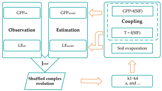
Figure 1.
Flowchart of model calibration.
3. Results
Scatter diagrams of modeled T ((a,d) TSLR estimated by the SLR method, (b,e) TWUE estimated by the WUE method, and (c, f) Tgs estimated by the conductance method) versus TZhou estimated by the uWUE method are shown in Figure 2. Both the WUE method and conductance method showed good performance at hourly (upper row) and daily (lower row) scales. In general, the conductance method outperformed the other two methods with higher coefficients of determination (R2) (0.67 for the hourly scale and 0.78 for the daily scale) and lower root-mean-square error (RMSE) (58.13 W/m2 for the hourly scale and 39.56 W/m2 for the daily scale). The SLR method and WUE method tended to overestimate T at the high-value area, while most points of the conductance method fell near the 1:1 line. All three methods showed better performance at the daily scale than the hourly scale, which could be attributed to the uncertainty of input data decreased with time aggregation. The difference in the performance of the SLR and WUE methods narrowed at the daily scale.
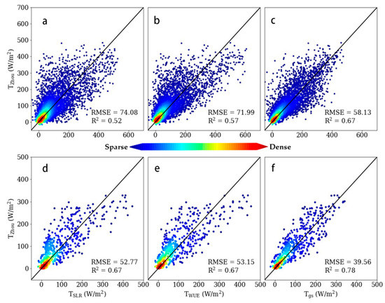
Figure 2.
Scatterplot of hourly (first row) and daily (second row) T estimates from the three approaches (linear method, water-use efficiency (WUE) method, and conductance method) versus Tzhou (estimated by underlying WUE method) with the 1:1 line (black line), along with coefficients of determination (R2) and root-mean-square error (RMSE, W/m2). Subfigures (a,d) refer to the linear method, (b,e) to the WUE method, and (c,f) to the conductance method.
As shown in Figure 3, we also compared the latent heat estimated by three different methods ((a,d) LESLR estimated by the SLR method, (b,e) LEWUE estimated by the WUE method, and (c,f) LEgs estimated by the conductance method) with latent heat observed from eddy covariance. Three methods had R2 = 0.56, 0.61, and 0.65 (RMSE = 91.36, 88.06, and 80.87 W/m2) at the hourly scale (upper row), and R2 = 0.52, 0.66, and 0.67 (RMSE = 75.17, 65.52, and 61.07 W/m2) at the daily scale (lower row), respectively. Likewise, two developed methods showed better performance than the SLR method at the hourly scale, and the leading advantage widened at the daily scale. There was also an overestimation at the high-value area for the SLR and WUE methods. Details of the performance at four sites are shown in supplementary Table S3.
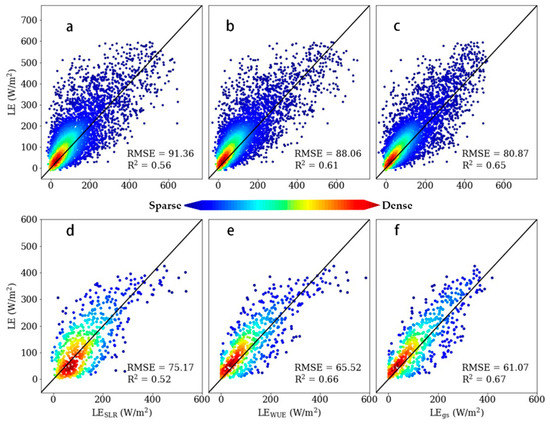
Figure 3.
Scatterplot of hourly (first row) and daily (second row) LE estimates from the three approaches (linear method, WUE method, and conductance method) versus LE (observed from eddy covariance) with the 1:1 line (black line), along with coefficients of determination (R2) and root-mean-square error (RMSE, W/m2). Subfigures (a,d) refer to the linear method, (b,e) to the WUE method, and (c,f) to the conductance method.
4. Discussion
4.1. Sensitivity Analysis of the Water-Use Efficiency (WUE) and Conductance Methods
To explore what influences the relationship between SIF and T, we analyzed the sensitivity of variables in the WUE and conductance methods. The scatterplots between SIF and TWUE for the four study sites are shown in Figure 4 (a, b, c, and d for hourly scale; e, f, g, and h for daily scale). T is the product of SIF and VPD in the WUE method, which means that SIF and VPD interact with each other closely and the effect of the SIF is modified by the VPD. The parameters k4 at the four sites were 0.33, 0.46, 1.00, and 0.11, respectively, at the hourly scale; and 0.10, 0.68, 1.00, and 0.25 at the daily scale. With the increase in VPD, the slopes of SIF–T became steeper and the points became denser, while under low VPD condition, the points were relatively sparse, which indicates that the relationship between SIF and T is more linear under high VPD. In particular, the relationship between SIF and T was strongly influenced by VPD at the NR site with evergreen needle leaf plants, but at the HF site, the SIF–T relationship was less sensitive to the VPD.
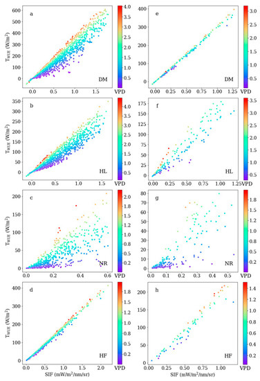
Figure 4.
Scatterplot between sun-induced chlorophyll fluorescence (SIF) and TWUE for the four study sites. Subfigures (a–d) for hourly scale; (e–h) for daily scale.
Atmospheric dryness also plays an important role in modeling the stomatal behavior by SIF. For C4 plants, relative humidity is used to describe the response of stomatal conductance to air dryness in the empirical Ball–Berry model. For C3 plants, we investigated the sensitivities of different variables in the gs model by RBD-FAST (Random Balance Designs-Fourier Amplitude Sensitivity Test) [58]. The results showed that was sensitive to VPD, λ, SIF, and qL (supplementary Figure S1). VPD exhibited the highest relative sensitivity of 0.34, which was much higher than SIF with a value of 0.17. The marginal water-use efficiency λ also played an important role with a sensitivity value equaling 0.32. The fraction of open Photosynthesis II reaction centers qL is as important as SIF (relative sensitivity of 0.17), which is due to the fact that the electron transport rate J is the product of SIF and qL (Equation (8)). Furthermore, the gs model is not sensitive to and Ca.
4.2. Uncertainty of the Developed Methods
Credible theoretical frameworks and external environmental variables were introduced to the developed methods to meet the challenges of modeling T by SIF. The WUE method links SIF and T from the carbon–water economy perspective, in which WUE is treated as a function of VPD. The conductance method clarifies how the information about J contained in SIF can be used to estimate gs, and the Penman–Monteith based on energy balance further combines the gs with other meteorological variables. The conductance method has a clearer physical meaning, which better describes the linkage between SIF and T. However, assumptions of optimal carbon–water coupling relationship, the uncertainty of input data, and the experimental design may also undermine the performance of the developed methods.
Compared with the simple linear regression method, though the influence of VPD on WUE is included in the WUE method, soil moisture, hydraulic conductance, and other environmental variables could also influence the WUE independently [15,59,60]. It would be helpful to incorporate the effects of these factors on WUE. For the conductance method, plants under stress or competition cannot keep the optimal stomatal conductance behavior [61,62]. The carbon–water economy is also influenced by traits of plants and environmental variables [63]. A more physiologically based water–carbon coupling framework will improve the models from the bottom up.
Uncertainty of the input data might also introduce uncertainty to the results. First, VPD of air above the canopy was used to assess the aridity stress by assuming the canopy and the atmosphere were fully coupled. Ecosystems with a dense closed-canopy tend to decouple from the air [64,65]. As both the WUE method and the conductance method show great sensitivity to VPD, using VPD at the leaf scale could help to improve the performance of the SIF–T relationship. Second, SIF data from four sites were measured by different instruments and derived by different methods as above-mentioned. Moreover, the field of view (FOV) and heights of the observation systems vary among different sites. The emergence of remotely sensed SIF will fill the gap in the difference in the observation data. The data during the period of cooling of Niwot Ridge were used in our research. However, during winter, water transport of the trees was blocked due to frozen bole [19]. Most stomata were closed and there was almost no transpiration and, to our knowledge, the carbon–water coupling relationship under physiological stress remains unclear. Moreover, the site was covered by snow during the winter, but the sublimation and melting process were not included in the evaporation model due to a lack in parameters about the snowpack, which might undermine the results of the NR site. Last but not least, the canopy-scale SIF was directly used to model T due to data restriction. Nevertheless, recent works indicated that the relationship between SIF and GPP is strongly affected by the structure of the canopy [66,67]. We suggest that downscaling SIF from the canopy scale to the photosystem scale may improve the performance of the developed methods.
Due to the absence of direct measurements of T during the study period, three models were calibrated by ET observed from EC. Net radiation is separated into energy intercepted by canopy and soil available energy by one dimensional Beer’s law. The simple structure of Beer’s law could introduce great uncertainty to energy partition, especially for heterogeneity canopy and plants with highly anisotropic leaves in the azimuthal direction [68], for example, maize at the early growing season at DM and HL sites. Canopy available energy was also used to estimate T in the two-layer Penman–Monteith model in the conductance method. Therefore, the conductance method is more sensitive to the partition of energy; in other words, it suffers more uncertainty from Beer’s law.
Data from only four sites were used to evaluate the performance of the developed methods. It is inadequate to show the real potential of the two methods. With more and more in situ observations from different ecosystems, understanding of the underlying mechanism between SIF and T will be deepened. Recently, SIF products with higher temporal-spatial resolution from different satellites, different bands [69,70], and derivative products based on machine learning [71,72,73,74] have become available. T can be estimated at larger scales with the WUE method and conductance method by combining remote-sensing SIF data with remote-sensing-based ET/T models like TSEB [75,76] and PML [77] or assimilating SIF into land surface models in future studies.
5. Conclusions
In this study, two mechanism methods, the WUE and stomatal conductance methods, were developed to estimate T via SIF observations. The two developed methods were tested at hourly and daily scales over four sites including two C3 sites and two C4 sites. Both methods showed good performance with higher R2 and lower RMSE, especially for the conductance method. Moreover, our results indicate that the SIF–T relationship strongly depends on air dryness. These two carbon–water coupling methods can be combined with state-of-the-art remote sensing models or land process models. With the emergence of high temporal-spatial resolution SIF data, SIF will not be only a powerful proxy for carbon flux, but also for water flux.
Supplementary Materials
The following are available online at https://www.mdpi.com/2072-4292/13/4/804/s1, Table S1: Input and intermediate variables, Table S2: Parameters needed to be calibrated, Table S3: Coefficient of determination and root mean square error of different SIF–T methods at different sites, Figure S1: Sensitivity analysis of variables in the stomatal conductance method of C3 plants. References [12,26,36,37,38,41,47,48,49,51,52,53,65] are cited in the Supplementary Materials.
Author Contributions
Conceptualization, T.X.; Formal analysis, H.F.; Investigation, L.L. and S.Z.; Methodology, J.Z., X.H., and Z.X.; Software, H.F.; Funding acquisition, S.L.; Validation, Z.Z. and L.C.; Visualization, T.X.; Writing, original draft preparation, H.F.; Writing, review and editing, L.L., S.Z., J.Z., X.H., T.X., S.L., Z.X., Z.Z., L.C., K.M., and H.F.; All authors have read and agreed to the published version of the manuscript.
Funding
This research was supported by the National Key Research and Development Program of China (2016YFC0500101) and the Strategic Priority Research Program of the Chinese Academy of Sciences (grant no. XDA20100101).
Institutional Review Board Statement
Not applicable.
Informed Consent Statement
Not applicable.
Data Availability Statement
The ground-measured sun-induced fluorescence data of the Daman and Huailai sites are available on Chinaspec (https://chinaspec.nju.edu.cn/). For the Niwot Ridge site, the SIF data were downloaded from CaltechDATA (https://data.caltech.edu/records/1231). Meteorological data and flux data were obtained from the National Tibetan Plateau Data Center (https://data.tpdc.ac.cn), Ameriflux (https://ameriflux.lbl.gov), and Harvard Forest Data Archive (https://harvardforest1.fas.harvard.edu). Leaf area index data of the four sites were extracted from Google Earth Engine (https://code.earthengine.google.com). Codes for this work are available on GitHub (https://github.com/Hydrometeorological-Remote-Sensing).
Acknowledgments
We would like to thank J. William Munger’s contributions in processing data from the EMS tower of Harvard Forest.
Conflicts of Interest
The authors declare no conflict of interest.
References
- Good, S.P.; Noone, D.; Bowen, G. Hydrologic connectivity constrains partitioning of global terrestrial water fluxes. Science 2015, 349, 175–177. [Google Scholar] [CrossRef] [PubMed]
- Jasechko, S.; Sharp, Z.D.; Gibson, J.J.; Birks, S.J.; Yi, Y.; Fawcett, P.J. Terrestrial water fluxes dominated by transpiration. Nat. Cell Biol. 2013, 496, 347–350. [Google Scholar] [CrossRef]
- Stoy, P.C.; El-Madany, T.S.; Fisher, J.B.; Gentine, P.; Gerken, T.; Good, S.P.; Klosterhalfen, A.; Liu, S.; Miralles, D.G.; Perez-Priego, O.; et al. Reviews and syntheses: Turning the challenges of partitioning ecosystem evaporation and transpiration into opportunities. Biogeosciences 2019, 16, 3747–3775. [Google Scholar] [CrossRef]
- Kool, D.; Agam, N.; Lazarovitch, N.; Heitman, J.; Sauer, T.; Ben-Gal, A. A review of approaches for evapotranspiration partitioning. Agric. For. Meteorol. 2014, 184, 56–70. [Google Scholar] [CrossRef]
- Ryu, Y.; Berry, J.A.; Baldocchi, D.D. What is global photosynthesis? History, uncertainties and opportunities. Remote Sens. Environ. 2019, 223, 95–114. [Google Scholar] [CrossRef]
- Schimel, D.; Schneider, F.D.; Participants, J.C. Flux towers in the sky: Global ecology from space. New Phytol. 2019, 224, 570–584. [Google Scholar] [CrossRef] [PubMed]
- Alemohammad, S.H.; Fang, B.; Konings, A.G.; Aires, F.; Green, J.K.; Kolassa, J.; Miralles, D.G.; Prigent, C.; Gentine, P. Water, energy, and carbon with Artificial Neural Networks (WECANN): A statistically based estimate of global surface turbulent fluxes and gross primary productivity using solar-induced fluorescence. Biogeosciences 2017, 14, 4101–4124. [Google Scholar] [CrossRef] [PubMed]
- Jonard, F.; De Cannière, S.; Brüggemann, N.; Gentine, P.; Gianotti, D.S.; Lobet, G.; Miralles, D.; Montzka, C.; Pagán, B.; Rascher, U.; et al. Value of sun-induced chlorophyll fluorescence for quantifying hydrological states and fluxes: Current status and challenges. Agric. For. Meteorol. 2020, 291, 108088. [Google Scholar] [CrossRef]
- Lu, X.; Liu, Z.; An, S.; Miralles, D.G.; Maes, W.; Liu, Y.; Tang, J. Potential of solar-induced chlorophyll fluorescence to estimate transpiration in a temperate forest. Agric. For. Meteorol. 2018, 252, 75–87. [Google Scholar] [CrossRef]
- Pagán, B.R.; Maes, W.H.; Gentine, P.; Martens, B.; Miralles, D.G. Exploring the potential of satellite solar-induced fluorescence to constrain global transpiration estimates. Remote Sens. 2019, 11, 413. [Google Scholar] [CrossRef]
- Maes, W.H.; Pagán, B.R.; Martens, B.; Gentine, P.; Guanter, L.; Steppe, K.; Verhoest, N.E.; Dorigo, W.; Li, X.; Xiao, J.; et al. Sun-induced fluorescence closely linked to ecosystem transpiration as evidenced by satellite data and radiative transfer models. Remote Sens. Environ. 2020, 249, 112030. [Google Scholar] [CrossRef]
- Gu, L.; Han, J.; Wood, J.D.; Chang, C.Y.; Sun, Y. Sun-induced CHL fluorescence and its importance for biophysical modeling of photosynthesis based on light reactions. New Phytol. 2019, 223, 1179–1191. [Google Scholar] [CrossRef]
- Zhang, Y.; Guanter, L.; Berry, J.A.; Joiner, J.; Van der Tol, C.; Huete, A.; Gitelson, A.; Voigt, M.; Köhler, P. Estimation of vegetation photosynthetic capacity from space-based measurements of chlorophyll fluorescence for terrestrial biosphere models. Glob. Chang. Biol. 2014, 20, 3727–3742. [Google Scholar] [CrossRef] [PubMed]
- Wolz, K.J.; Wertin, T.M.; Abordo, M.; Wang, D.; Leakey, A.D.B. Diversity in stomatal function is integral to modelling plant carbon and water fluxes. Nat. Ecol. Evol. 2017, 1, 1292–1298. [Google Scholar] [CrossRef]
- Leakey, A.D.; Ferguson, J.N.; Pignon, C.P.; Wu, A.; Jin, Z.; Hammer, G.L.; Lobell, D.B. Water use efficiency as a constraint and target for improving the resilience and productivity of C3and C4Crops. Annu. Rev. Plant Biol. 2019, 70, 781–808. [Google Scholar] [CrossRef] [PubMed]
- Berry, J.A.; Beerling, D.J.; Franks, P.J. Stomata: Key players in the earth system, past and present. Curr. Opin. Plant Biol. 2010, 13, 232–239. [Google Scholar] [CrossRef]
- Shan, N.; Ju, W.; Migliavacca, M.; Martini, D.; Guanter, L.; Chen, J.; Goulas, Y.; Zhang, Y. Modeling canopy conductance and transpiration from solar-induced chlorophyll fluorescence. Agric. For. Meteorol. 2019, 268, 189–201. [Google Scholar] [CrossRef]
- Liu, X.; Liu, L.; Hu, J.; Guo, J.; Du, S. Improving the potential of red SIF for estimating GPP by downscaling from the canopy level to the photosystem level. Agric. For. Meteorol. 2020, 281, 107846. [Google Scholar] [CrossRef]
- Magney, T.S.; Bowling, D.R.; Logan, B.A.; Grossmann, K.; Stutz, J.; Blanken, P.D.; Burns, S.P.; Cheng, R.; Garcia, M.A.; Kç hler, P.; et al. Mechanistic evidence for tracking the seasonality of photosynthesis with solar-induced fluorescence. Proc. Natl. Acad. Sci. USA 2019, 116, 11640–11645. [Google Scholar] [CrossRef]
- Yang, X.; Tang, J.; Mustard, J.F.; Lee, J.-E.; Rossini, M.; Joiner, J.; Munger, J.W.; Kornfeld, A.; Richardson, A.D. Solar-induced chlorophyll fluorescence that correlates with canopy photosynthesis on diurnal and seasonal scales in a temperate deciduous forest. Geophys. Res. Lett. 2015, 42, 2977–2987. [Google Scholar] [CrossRef]
- Myneni, R.; Knyazikhin, Y.; Park, T. MCD15A3H MODIS/Terra+ Aqua Leaf Area Index/FPAR 4-day L4 Global 500m SIN Grid V006. NASA EOSDIS Land Processes DAAC. 2015. Available online: https://lpdaac.usgs.gov/products/mcd15a3hv006/ (accessed on 19 February 2021).
- Gorelick, N.; Hancher, M.; Dixon, M.; Ilyushchenko, S.; Thau, D.; Moore, R. Google earth engine: Planetary-scale geospatial analysis for everyone. Remote Sens. Environ. 2017, 202, 18–27. [Google Scholar] [CrossRef]
- Medlyn, B.E.; Duursma, R.A.; Eamus, D.; Ellsworth, D.S.; Prentice, I.C.; Barton, C.V.M.; Crous, K.Y.; De Angelis, P.; Freeman, M.; Wingate, L. Reconciling the optimal and empirical approaches to modelling stomatal conductance. Glob. Chang. Biol. 2011, 17, 2134–2144. [Google Scholar] [CrossRef]
- Zhou, S.; Yu, B.; Zhang, Y.; Huang, Y.; Wang, G. Partitioning evapotranspiration based on the concept of underlying water use efficiency. Water Resour. Res. 2016, 52, 1160–1175. [Google Scholar] [CrossRef]
- Zhou, S.; Yu, B.; Zhang, Y.; Huang, Y.; Wang, G. Water use efficiency and evapotranspiration partitioning for three typical ecosystems in the Heihe River Basin, northwestern China. Agric. For. Meteorol. 2018, 2018, 261–273. [Google Scholar] [CrossRef]
- Bai, Y.; Li, X.; Zhou, S.; Yang, X.; Yu, K.; Wang, M.; Liu, S.; Wang, P.; Wu, X.; Wang, X.; et al. Quantifying plant transpiration and canopy conductance using eddy flux data: An underlying water use efficiency method. Agric. For. Meteorol. 2019, 271, 375–384. [Google Scholar] [CrossRef]
- Massmann, A.; Gentine, P.; Lin, C. When does vapor pressure deficit drive or reduce evapotranspiration? J. Adv. Model. Earth Syst. 2019, 11, 3305–3320. [Google Scholar] [CrossRef]
- Liu, S.; Li, X.; Xu, Z.; Che, T.; Xiao, Q.; Ma, M.; Liu, Q.; Jin, R.; Guo, J.; Wang, L.; et al. The heihe integrated observatory network: A basin-scale land surface processes observatory in China. Vadose Zone J. 2018, 17, 180072. [Google Scholar] [CrossRef]
- Liu, S.M.; Xu, Z.W.; Wang, W.Z.; Jia, Z.Z.; Zhu, M.J.; Bai, J.; Wang, J.M. A comparison of eddy-covariance and large aperture scintillometer measurements with respect to the energy balance closure problem. Hydrol. Earth Syst. Sci. 2011, 15, 1291–1306. [Google Scholar] [CrossRef]
- Liu, X.; Guo, J.; Hu, J.; Liu, L. Atmospheric Correction for tower-based solar-induced chlorophyll fluorescence observations at O2-A band. Remote Sens. 2019, 11, 355. [Google Scholar] [CrossRef]
- Guo, A.; Liu, S.; Zhu, Z.; Xu, Z.; Xiao, Q.; Ju, Q.; Zhang, Y.; Yang, X. Impact of lake/reservoir expansion and shrinkage on energy and water vapor fluxes in the surrounding area. J. Geophys. Res. Atmos. 2020, 125. [Google Scholar] [CrossRef]
- Liu, S.; Xu, Z.; Zhu, Z.; Jia, Z.; Zhu, M. Measurements of evapotranspiration from eddy-covariance systems and large aperture scintillometers in the Hai River Basin, China. J. Hydrol. 2013, 487, 24–38. [Google Scholar] [CrossRef]
- Burns, S.P.; Blanken, P.D.; Turnipseed, A.A.; Hu, J.; Monson, R.K. The influence of warm-season precipitation on the diel cycle of the surface energy balance and carbon dioxide at a Colorado subalpine forest site. Biogeosciences 2015, 12, 7349–7377. [Google Scholar] [CrossRef]
- Monson, R.K.; Turnipseed, A.A.; Sparks, J.P.; Harley, P.C.; Scott Denton, L.E.; Sparks, K.; Huxman, T.E. Carbon sequestration in a high elevation, subalpine forest. Glob. Chang. Biol. 2002, 8, 459–478. [Google Scholar] [CrossRef]
- Munger, W.; Wofsy, S. Canopy-Atmosphere Exchange of Carbon, Water and Energy at Harvard Forest Ems Tower Since 1991; HF004; Harvard Forest Data Archive: Petersham, MA, USA, 2020. [Google Scholar]
- Guanter, L.; Zhang, Y.; Jung, M.; Joiner, J.; Voigt, M.; Berry, J.A.; Frankenberg, C.; Huete, A.R.; Zarco-Tejada, P.; Lee, J.-E.; et al. Global and time-resolved monitoring of crop photosynthesis with chlorophyll fluorescence. Proc. Natl. Acad. Sci. USA 2014, 111, E1327–E1333. [Google Scholar] [CrossRef]
- Liu, L.; Guan, L.; Liu, X. Directly estimating diurnal changes in GPP for C3 and C4 crops using far-red sun-induced chlorophyll fluorescence. Agric. For. Meteorol. 2017, 232, 1–9. [Google Scholar] [CrossRef]
- Sun, Y.; Frankenberg, C.; Jung, M.; Joiner, J.; Guanter, L.; Köhler, P.; Magney, T. Overview of Solar-Induced chlorophyll Fluorescence (SIF) from the Orbiting Carbon Observatory-2: Retrieval, cross-mission comparison, and global monitoring for GPP. Remote Sens. Environ. 2018, 209, 808–823. [Google Scholar] [CrossRef]
- Huang, M.; Piao, S.; Zeng, Z.; Peng, S.; Ciais, P.; Cheng, L.; Mao, J.; Poulter, B.; Shi, X.; Yao, Y.; et al. Seasonal responses of terrestrial ecosystem water-use efficiency to climate change. Glob. Chang. Biol. 2016, 22, 2165–2177. [Google Scholar] [CrossRef] [PubMed]
- Beer, C.; Ciais, P.; Reichstein, M.; Baldocchi, D.; Law, B.E.; Papale, D.; Soussana, J.-F.; Ammann, C.; Buchmann, N.; Frank, D.; et al. Temporal and among-site variability of inherent water use efficiency at the ecosystem level. Glob. Biogeochem. Cycles 2009, 23. [Google Scholar] [CrossRef]
- Zhou, S.; Yu, B.; Huang, Y.; Wang, G. The effect of vapor pressure deficit on water use efficiency at the subdaily time scale. Geophys. Res. Lett. 2014, 41, 5005–5013. [Google Scholar] [CrossRef]
- Magney, T.S.; Barnes, M.L.; Yang, X. On the covariation of chlorophyll fluorescence and photosynthesis across scales. Geophys. Res. Lett. 2020, 47. [Google Scholar] [CrossRef]
- Damm, A.; Guanter, L.; Paul-Limoges, E.; Van Der Tol, C.; Hueni, A.; Buchmann, N.; Eugster, W.; Ammann, C.; Schaepman, M.E. Far-red sun-induced chlorophyll fluorescence shows ecosystem-specific relationships to gross primary production: An assessment based on observational and modeling approaches. Remote Sens. Environ. 2015, 166, 91–105. [Google Scholar] [CrossRef]
- Zhang, Z.; Zhang, Y.; Porcar-Castell, A.; Joiner, J.; Guanter, L.; Yang, X.; Migliavacca, M.; Ju, W.; Sun, Z.; Chen, S.; et al. Reduction of structural impacts and distinction of photosynthetic pathways in a global estimation of GPP from space-borne solar-induced chlorophyll fluorescence. Remote Sens. Environ. 2020, 240, 111722. [Google Scholar] [CrossRef]
- Baker, N.R. Chlorophyll fluorescence: A probe of photosynthesis in vivo. Annu. Rev. Plant Biol. 2008, 59, 89–113. [Google Scholar] [CrossRef]
- Ball, J.T.; Woodrow, I.E.; Berry, J.A. A. A model predicting stomatal conductance and its contribution to the control of photosynthesis under different environmental conditions. In Progress in Photosynthesis Research; Springer International Publishing: Geneva, Switzerland, 1987; pp. 221–224. [Google Scholar]
- Miner, G.L.; Bauerle, W.L.; Baldocchi, D.D. Estimating the sensitivity of stomatal conductance to photosynthesis: A review. Plant Cell Environ. 2017, 40, 1214–1238. [Google Scholar] [CrossRef]
- Katul, G.; Manzoni, S.; Palmroth, S.; Oren, R. A stomatal optimization theory to describe the effects of atmospheric CO2 on leaf photosynthesis and transpiration. Ann. Bot. 2009, 105, 431–442. [Google Scholar] [CrossRef]
- Cowan, I.R.; Farquhar, G.D. Stomatal function in relation to leaf metabolism and environment. Symp. Soc. Exp. Biol. 1977, 31, 471–505. [Google Scholar]
- Way, D.A.; Katul, G.G.; Manzoni, S.; Vico, G. Increasing water use efficiency along the C3 to C4 evolutionary pathway: A stomatal optimization perspective. J. Exp. Bot. 2014, 65, 3683–3693. [Google Scholar] [CrossRef]
- Leuning, R.; Zhang, Y.Q.; Rajaud, A.; Cleugh, H.; Tu, K. A simple surface conductance model to estimate regional evaporation using MODIS leaf area index and the Penman-Monteith equation. Water Resour. Res. 2008, 44. [Google Scholar] [CrossRef]
- Nieto, H.; Guzinski, R.; Graae, P.; Jonas. ClaireBrenner hectornieto/pyTSEB v2.0, Zenodo. 2019. Available online: https://zenodo.org/record/48461#.YDYX42hKhPY (accessed on 19 February 2021). [CrossRef]
- Wang, H.; Ma, M. Estimation of transpiration and evaporation of different ecosystems in an inland river basin using remote sensing data and the Penman-Monteith equation. Acta Ecol. Sin. 2014, 34, 5617–5626. [Google Scholar]
- Duan, Q.; Sorooshian, S.; Gupta, V.K. Optimal use of the SCE-UA global optimization method for calibrating watershed models. J. Hydrol. 1994, 158, 265–284. [Google Scholar] [CrossRef]
- Harris, C.R.; Millman, K.J.; Van Der Walt, S.J.; Gommers, R.; Virtanen, P.; Cournapeau, D.; Wieser, E.; Taylor, J.; Berg, S.; Smith, N.J.; et al. Array programming with NumPy. Nature 2020, 585, 357–362. [Google Scholar] [CrossRef] [PubMed]
- Houska, T.; Kraft, P.; Chamorro-Chavez, A.; Breuer, L. SPOTting model parameters using a ready-made python package. PLoS ONE 2015, 10, e0145180. [Google Scholar] [CrossRef]
- Herman, J.; Usher, W. SALib: An open-source Python library for Sensitivity Analysis. J. Open Source Softw. 2017, 2, 97. [Google Scholar] [CrossRef]
- Tarantola, S.; Gatelli, D.; Mara, T.A. Random balance designs for the estimation of first order global sensitivity indices. Reliab. Eng. Syst. Saf. 2006, 91, 717–727. [Google Scholar] [CrossRef]
- Lin, Y.-S.; Medlyn, B.E.; Duursma, R.A.; Prentice, I.C.; Wang, H.; Baig, S.; Eamus, D.; De Dios, V.R.; Mitchell, P.J.; Ellsworth, D.S.; et al. Optimal stomatal behaviour around the world. Nat. Clim. Chang. 2015, 5, 459–464. [Google Scholar] [CrossRef]
- Liu, Y.; Kumar, M.; Katul, G.G.; Feng, X.; Konings, A.G. Plant hydraulics accentuates the effect of atmospheric moisture stress on transpiration. Nat. Clim. Chang. 2020, 10, 691–695. [Google Scholar] [CrossRef]
- Bloom, A.J.; Chapin, F.S., III; Mooney, H.A. Resource limitation in plants—An economic analogy. Annu. Rev. Ecol. Syst. 1985, 16, 363–392. [Google Scholar] [CrossRef]
- Wolf, A.; Anderegg, W.R.L.; Pacala, S.W. Optimal stomatal behavior with competition for water and risk of hydraulic impairment. Proc. Natl. Acad. Sci. USA 2016, 113, E7222–E7230. [Google Scholar] [CrossRef]
- Buckley, T.N.; Sack, L.; Farquhar, G.D. Optimal plant water economy. Plant Cell Environ. 2017, 40, 881–896. [Google Scholar] [CrossRef]
- De Kauwe, M.G.; Medlyn, B.E.; Knauer, J.; Williams, C.A. Ideas and perspectives: How coupled is the vegetation to the boundary layer? Biogeosciences 2017, 14, 4435–4453. [Google Scholar] [CrossRef]
- Lin, C.; Gentine, P.; Huang, Y.; Guan, K.; Kimm, H.; Zhou, S. Diel ecosystem conductance response to vapor pressure deficit is suboptimal and independent of soil moisture. Agric. For. Meteorol. 2018, 250, 24–34. [Google Scholar] [CrossRef]
- Liu, X.; Guanter, L.; Liu, L.; Damm, A.; Malenovský, Z.; Rascher, U.; Peng, D.; Du, S.; Gastellu-Etchegorry, J.-P. Downscaling of solar-induced chlorophyll fluorescence from canopy level to photosystem level using a random forest model. Remote Sens. Environ. 2019, 231, 110772. [Google Scholar] [CrossRef]
- Zeng, Y.; Badgley, G.; Dechant, B.; Ryu, Y.; Chen, M.; Berry, J. A practical approach for estimating the escape ratio of near-infrared solar-induced chlorophyll fluorescence. Remote Sens. Environ. 2019, 232, 111209. [Google Scholar] [CrossRef]
- Ponce De León, M.A.; Bailey, B.N. Evaluating the use of Beer’s law for estimating light interception in canopy architectures with varying heterogeneity and anisotropy. Ecol. Model. 2019, 406, 133–143. [Google Scholar] [CrossRef]
- Du, S.; Liu, L.; Liu, X.; Zhang, X.; Zhang, X.; Bi, Y.; Zhang, L. Retrieval of global terrestrial solar-induced chlorophyll fluorescence from TanSat satellite. Sci. Bull. 2018, 63, 1502–1512. [Google Scholar] [CrossRef]
- Köehler, P.; Frankenberg, C.; Magney, T.S.; Guanter, L.; Joiner, J.; Landgraf, J. Global retrievals of solar-induced chlorophyll fluorescence with Tropomi: First results and intersensor comparison to OCO-2. Geophys. Res. Lett. 2018, 45. [Google Scholar] [CrossRef]
- Li, X.; Xiao, J. A Global, 0.05-degree product of solar-induced chlorophyll fluorescence derived from OCO-2, MODIS, and reanalysis data. Remote Sens. 2019, 11, 517. [Google Scholar] [CrossRef]
- Ma, Y.; Liu, L.; Chen, R.; Du, S.; Liu, X. Generation of a Global spatially continuous tansat solar-induced chlorophyll fluorescence product by considering the impact of the solar radiation intensity. Remote Sens. 2020, 12, 2167. [Google Scholar] [CrossRef]
- Yu, L.; Wen, J.; Chang, C.Y.; Frankenberg, C.; Sun, Y. High-resolution global contiguous SIF of OCO-2. Geophys. Res. Lett. 2019, 46, 1449–1458. [Google Scholar] [CrossRef]
- Zhang, Y.; Joiner, J.; Alemohammad, S.H.; Zhou, S.; Gentine, P. A global spatially contiguous solar-induced fluorescence (CSIF) dataset using neural networks. Biogeosciences 2018, 15, 5779–5800. [Google Scholar] [CrossRef]
- Norman, J.M.; Kustas, W.P.; Humes, K.S. Source approach for estimating soil and vegetation energy fluxes in observations of directional radiometric surface temperature. Agric. For. Meteorol. 1995, 77, 263–293. [Google Scholar] [CrossRef]
- Song, L.; Kustas, W.P.; Liu, S.; Colaizzi, P.D.; Nieto, H.; Xu, Z.; Ma, Y.; Li, M.; Xu, T.; Agam, N.; et al. Applications of a thermal-based two-source energy balance model using Priestley-Taylor approach for surface temperature partitioning under advective conditions. J. Hydrol. 2016, 540, 574–587. [Google Scholar] [CrossRef]
- Zhang, Y.; Kong, D.; Gan, R.; Chiew, F.H.; McVicar, T.R.; Zhang, Q.; Yang, Y. Coupled estimation of 500 m and 8-day resolution global evapotranspiration and gross primary production in 2002–2017. Remote Sens. Environ. 2019, 222, 165–182. [Google Scholar] [CrossRef]


Publisher’s Note: MDPI stays neutral with regard to jurisdictional claims in published maps and institutional affiliations. |
© 2021 by the authors. Licensee MDPI, Basel, Switzerland. This article is an open access article distributed under the terms and conditions of the Creative Commons Attribution (CC BY) license (http://creativecommons.org/licenses/by/4.0/).