Article

Multi-Feature Fusion for Weak Target Detection on Sea-Surface Based on FAR Controllable Deep Forest Model

1
Department of Spaceborne Microwave Remote Sensing System, Aerospace Information Research Institute, Chinese Academy of Sciences, Beijing 100190, China
2
School of Electronics, Electrical and Communication Engineering, University of Chinese Academy of Sciences, Beijing 100049, China
*
Author to whom correspondence should be addressed.
Remote Sens. 2021, 13(4), 812; https://doi.org/10.3390/rs13040812
Submission received: 3 February 2021 / Revised: 16 February 2021 / Accepted: 18 February 2021 / Published: 23 February 2021

Abstract

:
Target detection on the sea-surface has always been a high-profile problem, and the detection of weak targets is one of the most difficult problems and the key issue under this problem. Traditional techniques, such as imaging, cannot effectively detect these types of targets, so researchers choose to start by mining the characteristics of the received echoes and other aspects for target detection. This paper proposes a false alarm rate (FAR) controllable deep forest model based on six-dimensional feature space for efficient and accurate detection of weak targets on the sea-surface. This is the first attempt at the deep forest model in this field. The validity of the model was verified on IPIX data, and the detection probability was compared with other proposed methods. Under the same FAR condition, the average detection accuracy rate of the proposed method could reach over 99.19%, which is 9.96% better than the results of the current most advanced method (K-NN FAR-controlled Detector). Experimental results show that multi-feature fusion and the use of a suitable detection framework have a positive effect on the detection of weak targets on the sea-surface.

Graphical Abstract

1. Introduction

Radar is an important tool for humans to explore the complex ocean. It plays an important role that cannot be ignored in ranging, detection, and surveillance and is of great significance in both military and civilian use. For example, navigation radar is often used to determine the position of other ships or floating objects on the sea-surface to ensure the safety of ships and avoid obstacles on the sea, etc [1]. Therefore, target detection is one of the important tasks of radar, and the detection technology of low observable targets in a complex environment has become a key constraint factor affecting radar performance [2,3]. Due to the low speed or small targets floating on the sea surface, such as buoys, iceberg debris, boats, floating objects, etc., which have the characteristics of small radar cross-section and low glancing angle, they have become the focus and difficulty in the target detection work of sea surface surveillance radar and ocean radar [4,5]. Although cooperative targets, such as large ships, are now equipped with an automatic identification system (AIS), which reduces the collision risk of cooperative ships, there is no guarantee that small ships and non-cooperative targets are equipped with AIS systems. Therefore, improving the detection capabilities of sea-surface surveillance radars and navigational radars on sea targets, especially low observable targets, is the key to ensuring the safe navigation of ships [6,7,8].
Since the continuous emergence of new types of targets and the iterative update of radar systems, radar detection technology on sea targets is a long-term topic and enduring. However, in view of the low observability of low-observable target itself and the need to quickly determine the existence of targets in the detection area, it is impossible to use common methods, such as imaging, for fast and effective target detection, so it is often necessary to use the characteristic difference between target echo signal and clutter echo signal to achieve efficient and accurate detection [9]. The characteristics of sea clutter are highly dependent on the sea state and the configuration of radar parameters. When the detection environment changes, the previously extracted features often lose robustness. Therefore, extracting robust features that adapt to changing environments from radar echoes is the key to target detection. In the early days, researchers focused on the amplitude or power characteristics of the echo. For instance, non-coherent statistical detection methods using the amplitude or power of radar echo and coherent processing detection algorithms based on echo complex data containing phase information and amplitude information.
A typical representative of non-coherent statistical detection methods is the constant false alarm rate (CFAR) proposed by Dugundji and John et al. This is a method that can automatically control the detector threshold. It enables the radar system to distinguish between the signal and noise output by the receiver while maintaining a constant false alarm probability whether the target signal exists [10,11,12]. On this basis, Steenson proposed a cell-average constant false alarm rate (CA-CFAR) detector. This is the optimal CFAR processor in a uniform background when the reference unit contains independent identically distributed (IID) observations controlled by exponential distribution [13,14]. In order to overcome the poor detection effect of CA-CFAR under the background of nonuniform noise, Hansen proposed the greatest of CFAR (GO-CFAR), using the greatest of the sums in the leading and lagging windows to estimate the noise power to adjust the clutter transition regional false alarm rate (FAR) [15]. However, GO-CFAR cannot distinguish targets that are closer. When an interfering target in the reference window has the same intensity as the main target, the detection probability of the detector will be significantly reduced [16]. Therefore, Trunk proposed the smallest of CFAR (SO-CFAR), which uses the minimum sum of the leading and lagging windows to estimate the noise power [17]. However, when the interfering target is in both leading and lagging windows, the detection performance of SO-CFAR will be greatly reduced, and SO-CFAR cannot keep the FAR a constant at the edge of clutter. The ordered statistic CFAR (OS-CFAR) detector proposed by Rohling alleviates these problems to a certain extent [16,18,19].
In essence, the core idea of the non-coherent detection method is the competition between the target energy and the surrounding clutter energy level, so it is simple to implement, and most of it is used in the early non-coherent system radar. With the advent of coherent radar, the received echo signal is a complex signal containing phase information and amplitude information so that people can coherently process the complex data. The typical one is the adaptive detection algorithm, which refers to a series of optimal or near-optimal coherent detectors developed based on a specific statistical model of sea clutter. In the case of small grazing angles, as the radar resolution increases, sea clutter can be modeled as a complex Gaussian distribution model. Based on this model, Kelly and Edward proposed the generalized likelihood ratio test [20], Fuhrmann and Daniel devised an adaptive matched filter (AMF) [21]. However, when the radar resolution is high, and the grazing angle is low, the Gaussian model is no longer applicable, and the sea clutter is modeled as a compound Gaussian model. Based on this model, Conte et al. proposed a normalized matched filter (NMF) detector [22], Richmond et al. proposed an adaptive normalized matched filter (ANMF) detector [23]. In view of the fact that the above methods are based on the spherical invariant random vector model and are suitable for short coherent accumulation time, they are often used for the detection of larger targets, such as surface ships and freighters, but when the target is small, or its speed is low, the target is often submerged in sea clutter, so the detection performance for low-observable targets on the sea surface is not very ideal.
In addition to coherent and incoherent statistical detection methods, there are also detection methods based on nonlinear modeling of sea clutter, such as sea surface fractal features detector. The fractal theory is a theory proposed by Mandelbrot in the 1970s to represent complex graphics and complex processes. Fractals can describe phenomena or substances with a certain degree of self-similarity at different scales from macro to micro in nature. The ocean surface is a complex dynamic rough surface of large-scale swells modulating small-scale capillary waves, which has certain fractal characteristics.
In 1993, T. Lo and others of McMaster University applied fractal theory to target detection under the background of sea clutter. By studying the measured data of sea clutter and according to the different fractal characteristics of the sea clutter and the target, a new target detection method was proposed, which breaks the limitation of the traditional energy-only detection method [24]. Subsequently, many scholars have deeply studied the difference of the fractal characteristics between sea clutter and the target echo and developed a series of related theoretical methods. In 2006, Hu Jing et al. introduced the multifractal theory based on structure–function. Through the analysis of 392 pieces of the sea clutter measured data, it was proposed that sea clutter data have multifractal characteristics in the time range of 0.01 s to several seconds, which can effectively detect low-observable targets on the sea surface [25]. Xu et al. used detrended fluctuation analysis (DFA) to extract the joint fractal characteristics of sea clutter, which provided valuable information for target detection [26]. Guan and Liu et al. derived the multifractal correlation spectrum from the multifractal theory and classified the target detection as a binary classification problem based on this feature. They used the support vector machine (SVM) for target detection. The experiment proved that this method has good weak target detection ability [27]. Fan and Luo used an autoregressive (AR) model to estimate the power spectrum of sea clutter, and studied its multifractal characteristics, proposed a local AR generalized Hurst exponent detection algorithm, and achieved good detection performance [28]. Besides this, He You and Guan Jian from the Naval Aviation University of China also introduced fractal theory into the frequency domain and fractional domain and proposed a method of typing detection based on the transform domain, providing new ideas for fractal detection [29,30].
When the state of the sea surface is unstable, the fractal dimension of the fractal feature will be unstable for a long time and in a large range. Therefore, the fractal theory has obvious limitations in detecting weak and small targets on the sea surface. Using only a fixed value as the detection threshold will lead to false alarms and missed alarms. Second, when the signal–clutter ratio (SCR) is at a low level, there is a little difference between sea clutter and target echo characteristics, so it is difficult to effectively detect weak targets on the sea-surface [4]. Modern radars often use linear frequency modulation (LFM) signals to generate signals with large time-bandwidth products. The time–frequency analysis method can better provide the joint information of the time domain and the frequency domain, so domestic and foreign scholars employed the time–frequency analysis to detect sea-surface targets.
Wang et al. analyzed the Doppler characteristics of sea clutter and proposed two target detectors; one was a Bayesian detector based on a joint Rayleigh distribution model, another one used entropy feature extracted from signal’s Doppler spectrum to build the detectors [31]. However, due to the changeable sea conditions, the Doppler spectrum of sea clutter often overlaps with that of small, low-speed targets. This single feature-based detector only uses limited return signal information, and its detection performance is easily affected by the change of the detection environment. Therefore, many researchers have proposed a feature fusion detection method that constructs a multidimensional feature space to obtain and utilizes more information from the return signal. First came Xu et al.’s two-dimensional convex hull detection algorithm based on sea clutter joint fractal features [26], followed by the Shui team’s three-dimensional feature detector based on the fast convex hull learning algorithm, they chose the three features of the relative average amplitude of received vector, relative Doppler peak height and relative entropy of Doppler amplitude spectrum to form the feature vector, and the measured data proved that this method could obtain better detection performance in second-level observation time [32].
However, in the case of low FAR and low SCR, the performance of these methods is restricted to varying degrees due to the resolution reduction of the time–frequency characteristics of the target echo. With the development of machine learning and deep learning, the robustness of detectors using deep learning as the advanced detection framework was further improved. Intelligent detection of low-observable targets on the sea surface combined with deep learning and time–frequency analysis has become a current research hotspot and research trend.
It is effective to select an appropriate deep learning method and use targeted features, such as effective information entropy in the case of low SCR, to obtain a detector with good detection performance and environmental robustness. The ability of such a constructed detector is demonstrated by the proposed method, SVM-based FAR controlled-detector [33], decision tree-based FAR controlled-detector [34], K-NN-based FAR controlled-detector [35]. Both the SVM-based and decision tree-based detectors use three features extracted from the echo signal to form a feature vector and are constructed by optimizing the detection framework with controllable FAR. The K-NN-based detector uses seven features extracted from the echo signal and used optimized K-NN as the detector. These detectors achieve exciting detection accuracy on the IPIX dataset, which is a significant improvement over the approach without the use of a deep learning framework. Inspired by these excellent methods, this article is dedicated to discovering more suitable feature spaces and model frameworks with better processing effects for small datasets.
(1) The choice of feature space. High-resolution sea clutter time-series contains abundant information on sea clutter and target. In this paper, six time–frequency features are selected from the proposed methods and extracted from the echo signal to form feature vectors, which are the relative mean amplitude (RMA) [32], the relative information entropy in the time domain (RIET) [34], the relative value of Doppler peak height (RPH) [32], the relative information entropy in Doppler domain (RIED) [32], the number of connected regions (NCR) [36] and the maximum size of connected regions (MSC) [36]. Moreover, optimized the selection method of RIET, NCR and MSC. They are the most representative features in the time domain, frequency domain, and time–frequency domain. They ensure the effectiveness of features under various conditions from multiple perspectives. The amplitude characteristics of the time domain and frequency domain can distinguish targets and clutter from the perspective of energy and spectrum differences. The information entropy features are not affected by changes in SCR, and features are still valid even under low SCR conditions. While the time–frequency domain feature uses the characteristic that the energy of the nonlinear frequency modulation signal can be completely concentrated on its instantaneous frequency curve to effectively distinguish the clutter from the target.
(2) The choice of detection framework. In the method proposed in this paper, gcForest [37] is selected as the base detection framework. The gcForest is an algorithm of deep forest. It is a novel ensemble model proposed by Zhou, a non-neural network (NN) style deep learning network. The algorithm is inspired by the construction of a deep neural network (DNN), extracts the idea of hierarchical data processing, and combines it with the cascading tree model. The model has the feature of automatically determining the number of training layers instead of a manual design before training so that the complexity of the model can be determined by relying on data. This allows gcForest to work well even on small-scale data and enables users to control training costs based on available computing resources. Moreover, it is high robustness to hyperparameter settings [37,38]. Furthermore, the tree classifier-based ensemble algorithm has more advantages than the NN class algorithm due to the natural class imbalance of the data. Based on the characteristics above, gcForest is very suitable to be used to deal with the current situation where there is fewer data available for training, and its parameter setting robustness also meets the requirements of robust detection. In addition, FAR is introduced as a threshold into the stop growth judgment condition of cascade level in gcForest. The stopping condition changes from a few rounds without significant improvement in training accuracy to a stop when the training result reaches the ideal FAR. If the expected conditions are not met, the model needs to continue training.
Based on this algorithm and combined with application scenarios, a FAR controllable gcForest is constructed. It is the first time that the deep forest model has been applied to the detection of weak targets on the sea surface. The introduction of multiple domain features weakens the detector’s sensitivity to changing environments. The addition of gcForest makes the detector fundamentally robust. The modification of gcForest improves the training speed to a certain extent, and the obtained model is more flexible and controllable. The detection accuracy of the method in this article and the proposed method are compared under the same FAR condition. The proposed method for comparison is shown below. A fractal-based detector [26] is a detector that uses the fractal and multifractal features of sea clutter to detect sea targets. Tri-feature-based detector [32], this detector extracts three features from the sea clutter and combines the fast convex hull learning algorithm to distinguish between the target and the clutter. TF-tri-feature-based detector [36], a detector that extracts three features from the time–frequency domain to construct the feature space and uses the convex hull algorithm to detect the target. Feature-compression-based detector [39], the detector extracts seven features from the echo to form a feature space, compresses the 7-D feature vector to 3-D, and uses an optimized, fast convex hull algorithm to detect the target cell. Moreover, the aforementioned detectors built using signal features and simple machine-learning methods, decision tree-based detector [34] and K-NN FAR-controlled detector [35]. The final comparison shows the method proposed in this paper achieves a higher detection probability based on achieving the same FAR.
The article structure is arranged as follows: Section 2 introduces the measured dataset used in the experiment, the features extracted from the data, and the structure of gcForest with controllable false alarms. Section 3 concisely gives the experimental results under different conditions. Section 4 discusses the network and the results obtained in the previous section in detail. Finally, the conclusion and some existing limitations are given in Section 5.

2. Materials and Methods

2.1. IPIX Dataset and Processing

The experiment uses IPIX measured data [40] for feature extraction. The IPIX radar is a portable numerical control coherent dual-polarization X-band radar used to detect the characteristics of sea clutter and the behavior of targets at different sea conditions. The research team of Professor Haykin of McMaster University collected the database of high-resolution radar measurements in November 1993. They used the radar called McMaster Intelligent Pixel Processing X-band (IPIX), which located at Osborne Head Gunnery Range, on the east coast of Canada, Dartmouth, Nova Scotia, facing the Atlantic Ocean, at the top of a cliff 100 feet above mean sea level, and had an open ocean view of about 130°. The collected data are typical small grazing angle radar data of a shore-based platform. The top view of the collection location and the radar picture are shown in Figure 1a,b [41]. The IPIX radar emits Horizontal polarization (H-polarization) and Vertical polarization (V-polarization) electromagnetic waves and receives radar echo data of four polarizations: two co-polarizations (HH polarization, VV polarization) and two cross polarizations (HV polarization, VH polarization). The parameters of IPIX are shown in Table 1.
There is a cooperative target in the irradiation area; it is a spherical Styrofoam block with a diameter of one meter, wrapped with wire mesh. The echo data consists of a time-series of length 2 17 and 14 distance units. As the radar illuminates the target at a low glancing angle, the target’s fluctuation and oscillation lead to the target’s energy diffusion, and the distance oversampling is adopted in the data collection, so the adjacent units around the target are affected by the target energy and are marked as affected units.
Since it contains cooperative targets and is equipped with an explicit description of the target existence unit and data records, such as wind speed and ocean waves at roughly the time of collection [42], many methods have used these data for experiments in recent years. The data used in this article are shown in Table 2. Due to the long time required, the description of the electromagnetic scattering characteristics of the cooperative target has not been found, so some documents on the study of the scattering characteristics of similar targets are supplemented for reference. The article [43] uses the reciprocity theorem to study the light scattering of spherical particles on the surface of a micro-rough nonuniform medium. The relationship between the surface roughness parameters and the position and size of the spherulites is also discussed in detail. The literature [44] uses Kirchhoff to approximate the backscattered field from the sea surface and analyzes the performance characteristics of the spherical target in the composite scattering field under different sizes and positions and different incident angles. The paper [45] uses Finite-difference time-domain (FDTD) to study the composite electromagnetic scattering characteristics of three-dimensional buoys and spherical targets above the sea surface. The changing law of scattering coefficient under the conditions of different incident angles, different sea surface wind speeds, drafts of pontoons and spheres is discussed in detail.
The SCR is the ratio of the signal power to the clutter power received by the radar. The target echo SCR can be estimated by the power of the range cell where the target is located. First, the average power p ¯ c of the sea clutter is estimated from the pure clutter unit in the echo. Assuming that the radar echo and sea clutter are independent, the average SCR can be estimated and solved using the following formulas:
A v e - S C R = 10 l g ( A ¯ p ¯ c ) ,
A ¯ = 1 N n = 1 N | x ( n ) | ,
where the x ( n ) represents the echo sequence of the unit where the target is located and N is the sequence length.
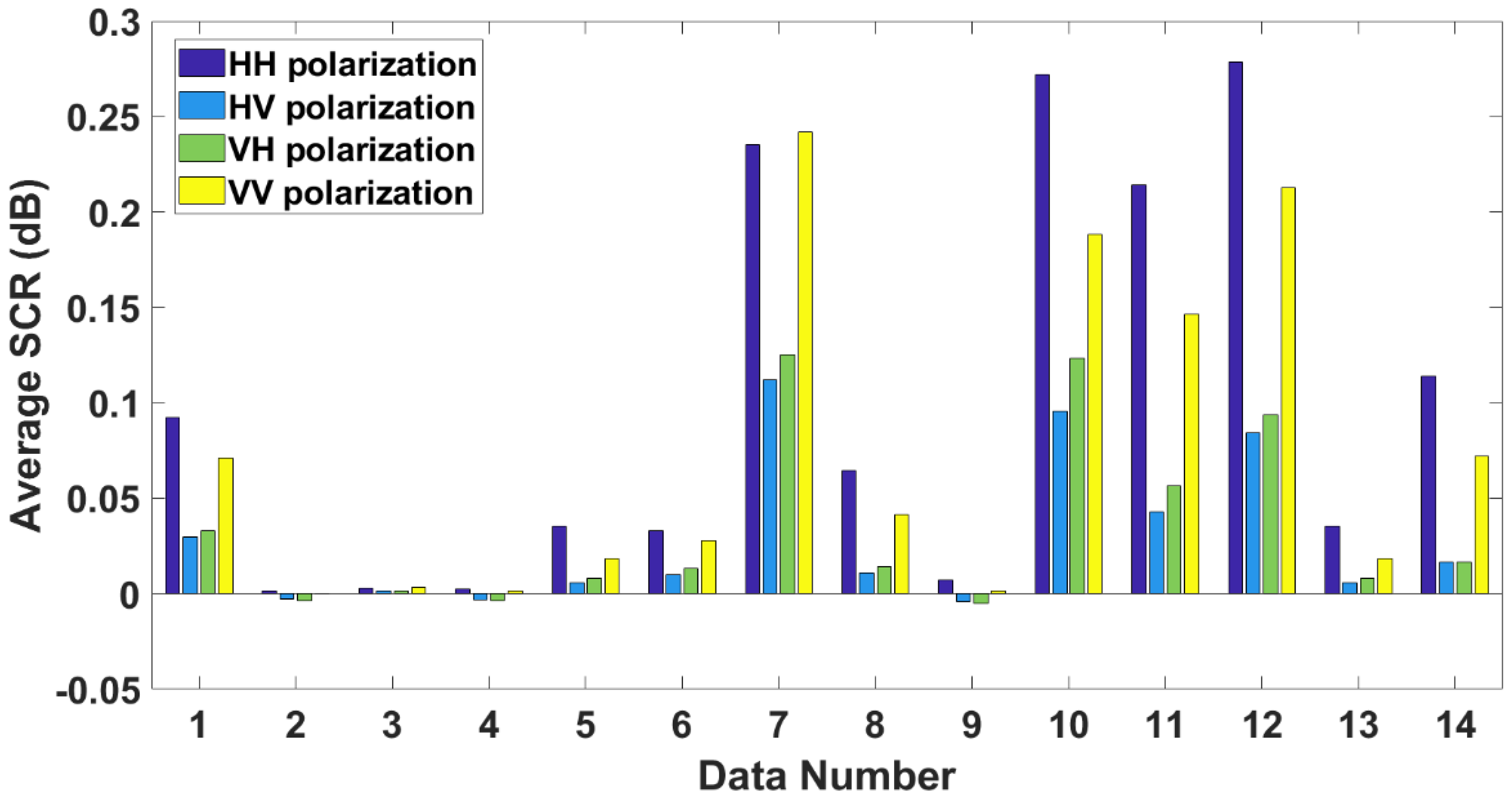
The fluctuation of the SCR is related to the difference in sea conditions, radar irradiation direction, target type, and polarization scattering characteristics. Lincoln Laboratory research shows that at low glancing angles, the sea clutter echo in the VV polarization mode is stronger than that in the HH polarization mode. The intensity ratio of the sea clutter between the VV polarization channel and the HH polarization channel increases with the increase of wavelength and decreases with the increase of sea conditions [46,47]. Figure 2 shows the target average SCR of the 14 sets of original data used in the experiment. It is not difficult to see that the difference between the Ave-SCR of the four polarizations is great. In most cases, the HH and VV have higher Ave-SCR than that of the other two cross-polarized Ave-SCRs, and due to the increase of sea conditions, the Ave-SCR of VV polarization and HH polarization is reduced, which is consistent with the previous research results.
As the target undulates and floats with the sea surface, when the glancing angles are low, there is a certain change in the target area radiated by the radar. The target is even blocked by the waves and cannot be reached by radar. Therefore, the actual SCR fluctuates and fluctuates to a certain extent near the average SCR.
The experiment in this paper selects the primary cell of targets and the clutter-only cell of the above 14 echo data as target signals and sea clutter signals, extracts six most representative features in the time–domain, frequency–domain and time–frequency domain to construct the feature vector. The validity of these features has been proven from multiple angles in published papers [32,33,34,35,36]. At the same time, it should be clear that no feature can guarantee its effectiveness under any circumstances. Therefore, this paper selected a variety of features to ensure the validity of the feature vectors under different conditions.

2.2. Features in Experiments

Since weak targets are easily affected by ocean waves, their motion characteristics are difficult to estimate. At this time, both the target signal and the sea clutter are non-stationary signals, and neither time-domain nor frequency-domain analysis alone can fully present the characteristics of both [48]. In addition, different features are sensitive to different levels of data, so detectors based on a single feature will not be suitable for every situation. In order to obtain better and more robust detection results, this paper extracts six representative features in time, frequency, and time–frequency domains based on the data collected by IPIX radar constructs a comprehensive and effective feature vector. First, select the amplitude feature in the time domain and frequency domain to provide a way to distinguish the target and clutter from the energy point of view. Second, the information entropy feature that is still valid under low SCR is selected to deal with the problem of extreme conditions. Finally, the signal and clutter exhibit completely different characteristics in the time–frequency domain, which can be used to assist in distinguishing them.
These six features are time-domain features: (1) relative mean amplitude (RMA), (2) relative information entropy in time-domain (RIET), (3) Doppler features (relative Doppler peak with high (RPH), (4)relative information entropy in Doppler-domain (RIED)), (5) time–frequency characteristics (the number of connected regions (NCR)) and (6) maximum size of the connected regions (MSC) extracted from the important time–frequency points (ITFP). The target detection problem is transformed into a binary classification problem by constructing a six-dimensional eigenvector composed of the above features.
Target detection in the background of sea clutter usually uses the following binary hypothesis test [49,50]:
{ H 0 : x ( n ) = c ( n ) H 1 : x ( n ) = s ( n ) + c ( n ) ,
where x ( n ) is the radar echo, s ( n ) is target echo, c ( n ) is sea clutter echo, n = 1 , 2 , , N is the number of radar transmitting pulses. In order to get more features, the echoes are divided into m segments with length d , the signal fragment is expressed as x sub = x ( w * ( m 1 ) + 1 : w * ( m 1 ) + d ) , w is an arbitrary integer so that there are some overlaps between sub-signals. The following feature analysis selects the HV polarization mode of the first data 19931107_135603_starea.

2.2.1. Relative Mean Amplitude

The relative magnitude of echo intensity is the main basis of traditional radar target detection. The relative mean amplitude (RMA) is the ratio of the average echo intensity of the main target cell to the average echo intensity of all pure clutter cells.
Suppose the length of echo time-series x is N , then the definition of the mean amplitude of echo is as follows,
A ¯ ( x ) = 1 N n = 1 N | x ( n ) | ,
A ¯ ( x ) is the mean value of the aim unit’s echo intensity, A ¯ ( x l ) is the mean value of the l - th clutter-only unit’s echo intensity, the calculation method of RMA is shown below
R M A ( x ) = A ¯ ( x ) 1 L l = 1 L A ¯ ( x l ) ,
for sea clutter with a non-stationary distance, averaging the clutter cell can make the RMA feature have a certain constant false alarm characteristic.
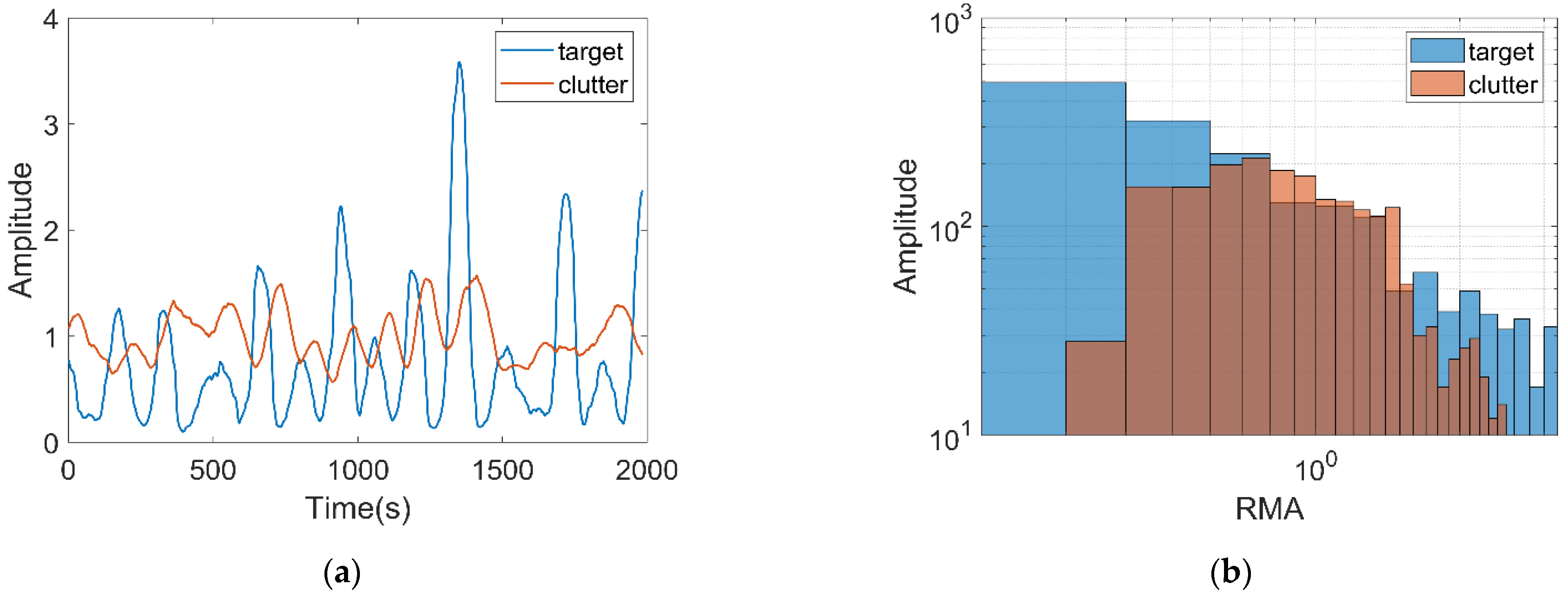
As can be seen from Figure 3a, it is impossible to distinguish the target and the clutter cell directly from the amplitude of the echo. Since the target fluctuates with the waves, its scattering characteristics vary greatly; the RMA of the target in Figure 3b is more dispersed than that of the clutter. Although there are some differences between the RMA distribution characteristics of clutter and targets, it is still impossible to detect the targets through a single RMA performance.

2.2.2. Relative Information Entropy in Time Domain

Information entropy can describe the uncertainty of random signals. In this paper, the concept of information entropy in information theory is introduced to describe the uncertainty of time-domain echo signals. Combined with the definition of information entropy, the information entropy of time-domain signal can be expressed as:
H s ( x ) = k = 1 K p ( n i ) l o g 2 p ( n i ) ,
and regulates 0 l o g 2 ( 0 ) = 0 . p ( n i ) is the probability that the signal falls in the amplitude interval of a range cell after dividing the amplitude into K equal parts:
p ( n i ) = n i N , i = 1 , 2 , , K ,
using L clutter cells as reference units, take the ratio of the information entropy between the target cell and the clutter-only cell, the relative information entropy in the time domain (RIET) is defined as:
R I T E ( x ) = H s ( x ) 1 L l = 1 L H s ( x l ) .
Figure 4a is RIET histogram; it is not difficult to find that due to the wave undulations, the cross-sectional radar area of the target also changes greatly, the echo signal has greater uncertainty; therefore, the RIET distribution of target echo is more divergent than that of the clutter-only cell. Figure 4b is a single-channel RIET of 11 echo cells (10 clutter-only cells and 1 target cell). It can be seen that the cell average RIET of target echo is larger than that of clutter-only echo. It is consistent with the theoretical analysis.

2.2.3. Relative Value of Doppler Peak Height

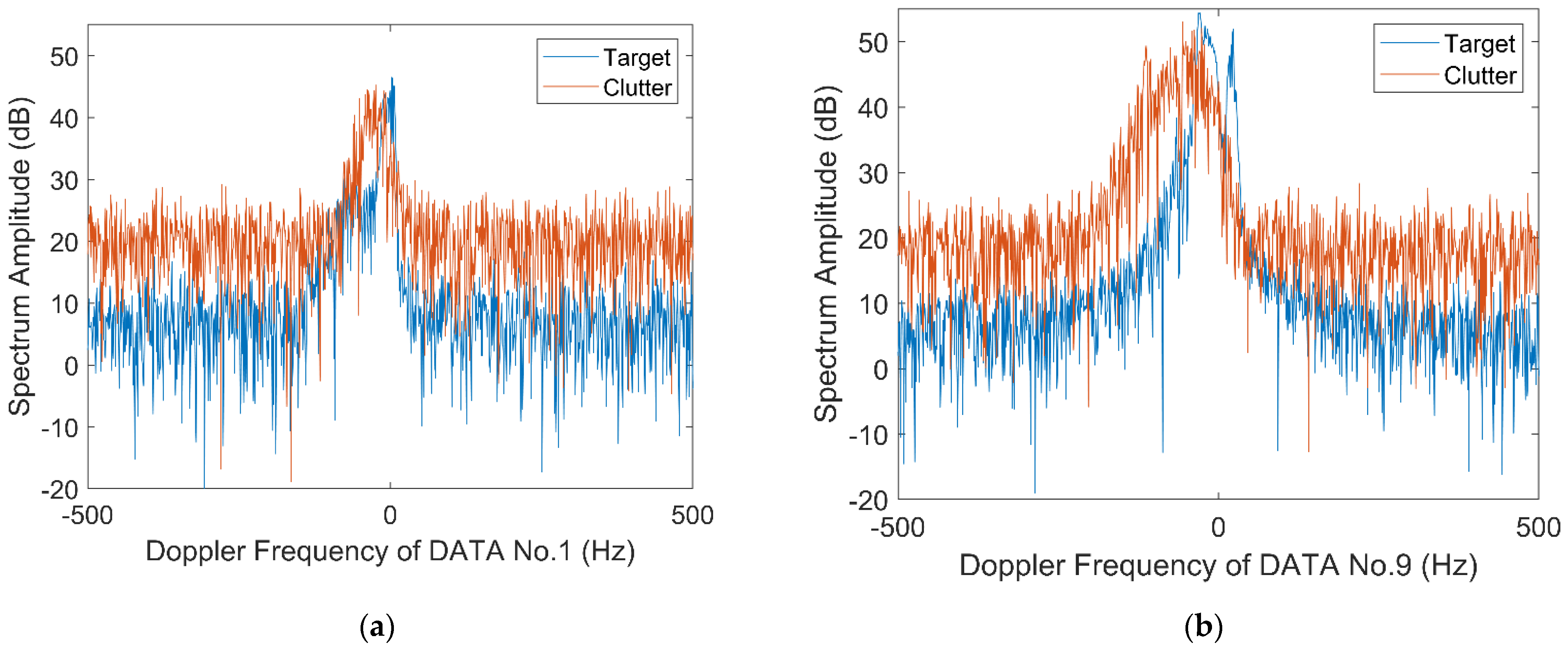
Due to the time-varying sea conditions, the sea surface under radar irradiation has different scattering structures, which leads to the wide Doppler bandwidth of sea clutter, while the Doppler peak of the weak target on the sea surface is easily submerged by the main clutter due to the small radial velocity. Figure 5 also confirms this problem. Therefore, it is difficult to separate the two by using absolute Doppler amplitude alone, so the influence of clutter Doppler bandwidth is eliminated by calculating the relative value of Doppler peak height (RPH) of target and clutter-only cell.
The calculation process of RPH is introduced below. First, find the Doppler peak height of the echo signal and its corresponding frequency point. T r = 0.001 is the pulse repetition frequency of IPIX radar,
P e a k ( x ) = max f d [ 1 / 2 T r , 1 / 2 T r ] ( X ( f d ) ) ,
f d m a x ( x ) = a r g   m a x f d [ 1 / 2 T r , 1 / 2 T r ] ( X ( f d ) ) ,
Next, the frequency domain reference cell σ is selected to calculate the one-dimension RPH, where δ 1 and δ 2 are the outer boundary and the inner boundary needed to calculate it, respectively. The role of these boundaries is to minimize the interference by excluding the bandwidth occupied by the target from the Doppler frequency domain, where the relative peak height is calculated. As shown in Formula (12), η ( x ) is the definition of RPH in a range cell, where N ( σ ) is the reference cell length,
σ = [ f d   m a x δ 1 , f d   m a x δ 2 ] [ f d   m a x + δ 2 , f d   m a x + δ 1 ] ,
η ( x ) = P e a k ( x ) 1 N ( σ ) f d σ X ( f d ) ,
According to experience, take δ 1 = 50 Hz, δ 2 = 5 Hz, using the cells to be estimated and L clutter reference cells, the RPH in the two-dimensional range, the Doppler plane is defined as follows:
R P H ( x ) = η ( x ) 1 L l = 1 L η ( x l ) ,
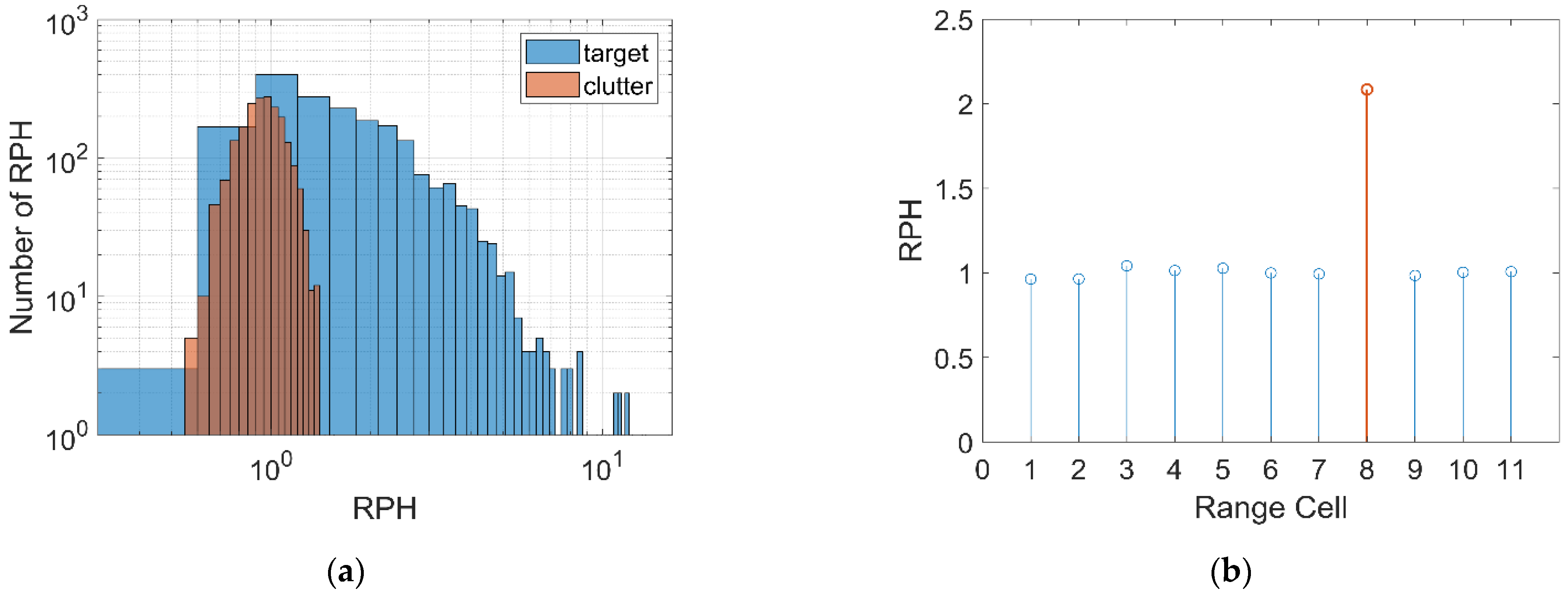
From the histogram of RPH in Figure 6a, it can be seen that the RPH value and distribution range of the target echo are bigger than that of the clutter-only echo. Figure 6b is the RPH of each echo cell; it is obvious that the average RPH of the target cell is much larger than that of each clutter-only cell, which also confirms the previous statement.

2.2.4. Relative Information Entropy in Doppler Domain

In Section 2.2.2, the time-domain amplitude characteristics of the echo signal are obtained by using information entropy. This part uses the information entropy to obtain the frequency-domain amplitude characteristics of the echo signal, and the presence of targets is detected by using the different energy distribution of the Doppler amplitude spectrum of the pure clutter cell and the target cell. With the foreshadowing, the relative information entropy of the Doppler domain (RIED) is defined as follows:
H s d ( x ) = f d X ^ ( f d ) l o g 2 X ^ ( f d ) ,
X ^ ( f d ) is the normalized Doppler amplitude spectrum
X ^ ( f d ) = X ( f d ) f d X ( f d ) ,
using L clutter cells as reference units, RIED is defined as
R I E D ( x ) = H s d ( x ) 1 L l = 1 L H s d ( x l ) ,
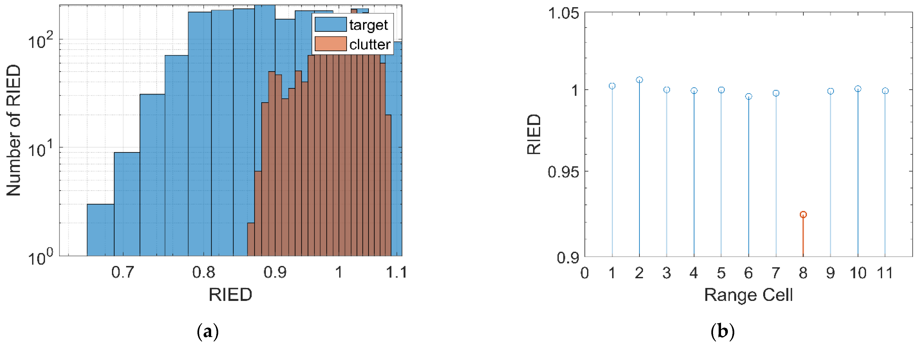
It can be seen from the histogram in Figure 7a that in the Doppler domain, the RIED distribution of clutter is more compact, but the overall value of the distribution is higher, while that of the target is more dispersed and most of the values are smaller than the clutter. Figure 7b is the single-channel RIED of 11 echo cells. The average RIED values of the clutter-only cells are relatively close, and they are greater than that of the target cell. The results show that the echo containing target appears completely different characteristics in the time-domain and Doppler-domain, and the Doppler spectrum of sea clutter is more chaotic.

2.2.5. The Number of Connected Regions and Maximum Size of Connected Regions

When analyzing the acquired signal, time–frequency analysis can obtain the signal’s time-varying frequency spectrum characteristics, which is a non-negligible feature and is called the micro-Doppler feature. For multicomponent signals in a high noise environment, scholars have proposed many methods to analyze time–frequency characteristics, such as using instantaneous frequency (IF) to obtain time–frequency information of the signals, using short-time Fourier transform, wavelet transforms, and so on to estimate the instantaneous frequency of the signals by using the linear time–frequency transform of short-time signals. Choi–Williams distribution (CWD) uses different kernel functions to suppress the cross term [51]. By designing a suitable kernel function, it can achieve greater attenuation of the cross term and satisfy time–frequency edge characteristics. The limited support loss in the time–frequency domain is better than other time–frequency analysis methods. Therefore, this paper calculates the normalized CWD to get the characteristics of its normalized time–frequency distribution: the number of connected regions and the maximum size of connected regions in the important time–frequency feature.
The CWD definition of the echo signal x ( t ) is as follows:
C W D x ( t , f ) = φ ( τ , ν ) A x ( τ , ν ) e x p ( j 2 π ( t ν f τ ) ) d τ d ν ,
φ ( τ , ν ) is the kernel function of time–frequency distribution of Cohen class, which is defined as Formula (19), A x ( τ , ν ) is the fuzzy function:
φ ( τ , ν ) = e τ 2 ν 2 σ ,
A x ( τ , ν ) = + x ( t + τ 2 ) x * ( t τ 2 ) e x p ( j 2 π t ν ) d t ,
When dealing with signals with large amplitude and frequency variation, the kernel function takes the larger σ ( σ > 1 ) ; otherwise, take the smaller σ ( σ 1 ) . When 0.1 σ 10 , Choi–Williams distribution can obtain a higher time–frequency resolution and can suppress more cross-terms [41]. In order to further eliminate the interference of the cross term, the time domain and frequency domain smoothing window is added in the CWD calculation. Therefore, the CWD of the complex time-series x = [ x ( 1 ) , x ( 2 ) , , x ( N ) ] T can be expressed as:
C W D x ( t , f | x ) = + g ( ν τ ) [ + h ( τ ) φ ( τ , ν ) A x ( τ , ν ) e x p ( j 2 π ( t ν f τ ) ) d τ ] d ν ,
Among them, g ( · ) and h ( · ) are time and frequency smoothing windows, respectively, the length of the time smoothing window g ( · ) is consistent with the max sampling interval of the target Doppler frequency, the selection of the frequency smoothing window h ( · ) is consistent with the signal division length of the chirp signal. The length of these two windows is related to the instantaneous frequency characteristics of the target and the sea condition. For IPIX radar data, the Doppler frequency of the cooperative target exhibits a pseudo-periodical behavior of about a few seconds. The target returns length to keep constant Doppler bias is about tens of milliseconds, and the length for target returns to keep constant Doppler rate of change is about a fraction of a second [37]. In addition, the Hamming window is good at reducing the nearest side lobe width; hence, in this paper, Hamming windows with time-domain length 125 and frequency domain length 255 are used. On the two-dimensional time–frequency plane, the CWD is normalized by using the mean function and standard deviation function of sea clutter to eliminate the non-stationarity of sea clutter time series in time and space.
N - C W D ˜ x ( t , f | x ) = C W D x ( t , f | x ) μ ^ ( t , f ) σ ^ ( t , f ) ,
where μ ^ ( t , f ) and σ ^ ( t , f ) are the mean and variance of clutter-only, respectively, and the calculation process is as follows:
μ ^ ( t , f ) = 1 L l = 1 L C W D x ( t , f | x ) ,
σ ^ ( t , f ) = 1 L 1 l = 1 L ( C W D x ( t , f | x l ) μ ^ ( t , f ) ) 2
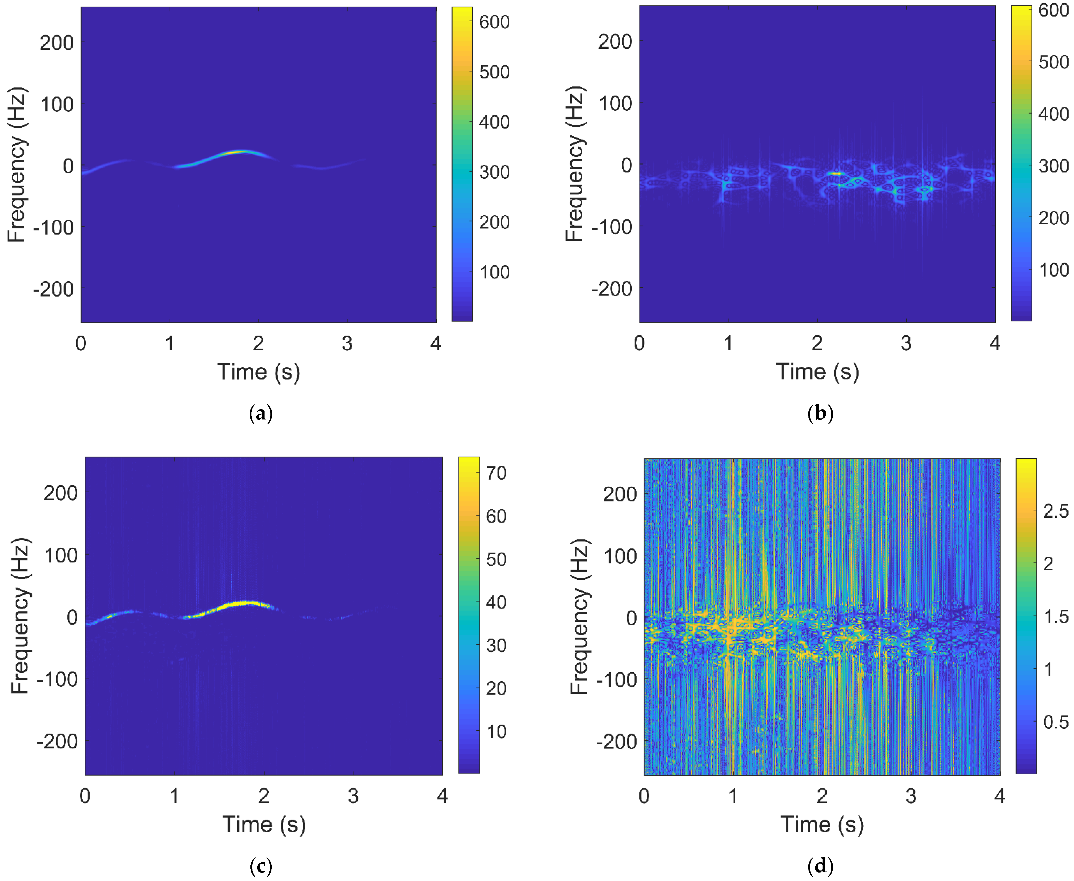
Figure 8a,b is the CWD of target echo and sea clutter. In the time–frequency plane, the energy of target echo is concentrated in a narrow band area, while the energy of clutter is concentrated in a band area. The brightness and width of the band area change with time and the frequency range is roughly from −100 Hz to 10 Hz. Figure 8c,d shows the Normalized-CWD (N-CWD) of the normalized target and sea clutter. After normalization, the echo energy of the target becomes more concentrated and becomes bright outside the clutter area, while the energy of sea clutter decreases significantly after normalization.
Next, time–frequency characteristics are extracted from N-CWD, and the maximum pixel values of the first K of the target echo and sea clutter in the time–frequency plane are marked as 1, and the remaining points are all set to zero to generate a binary image composed of the first K important time–frequency points (ITFP):
I T F P k = { 1 ( t , m a x k ( f ) )   i n   N - C W D ˜ x ( t , f | x ) 0 o t h e r s ,
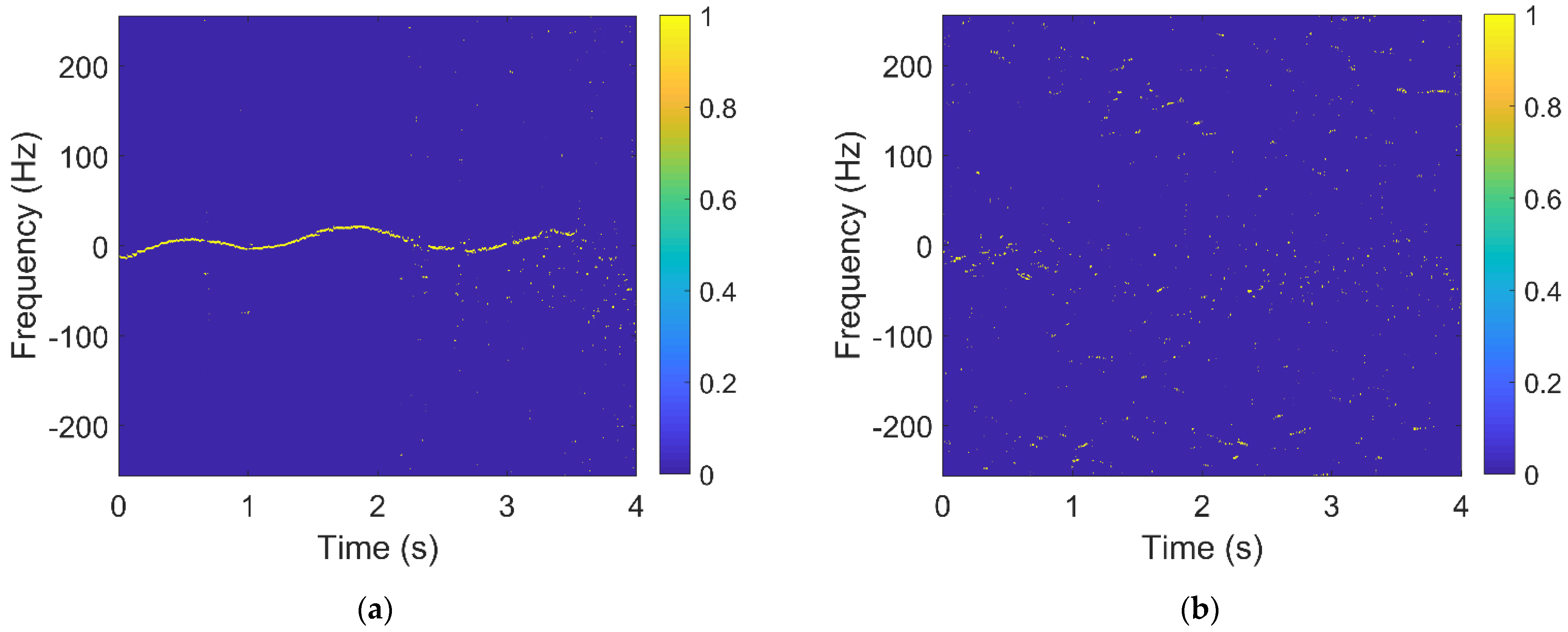
It can be seen from the image that the ITFP containing the target is highly clustered, while the ITPF image containing the pure clutter is scattered.
Based on the characteristics that the connected area of the target image is large, and the number of connected areas is small, the connected area of the clutter image is small, but the number of connected areas is large, two features, the number of connected regions (NCR) and maximum size of connected regions (MSC), are extracted from the image by using the principle of binary morphology. Mathematical morphology is applied to binary images, and the image is regarded as a set. To obtain these two features, it is necessary to find all the regions in the graph that meet the 4-connected or 8-connected conditions in this set. The number of pixel points contained in the region is the size of the connected region. If the connected region in a binary image is, then these two features are defined as follows:
{ N C R = S M S C = m a x k = 1 , 2 , , S { C R 1 , C R 2 , , C R k } ,
In Figure 9a, the STFP image of sea clutter contains a total of 3750 connected regions, of which the maximum area size is 317. In Figure 9b, the ITFP image of the target echo contains only 1212 connected regions, whose maximum area size is 3248. The ITFP images of sea clutter and target echo have obvious differences in these two features, so they can be used as features for target detection.

2.2.6. Summary

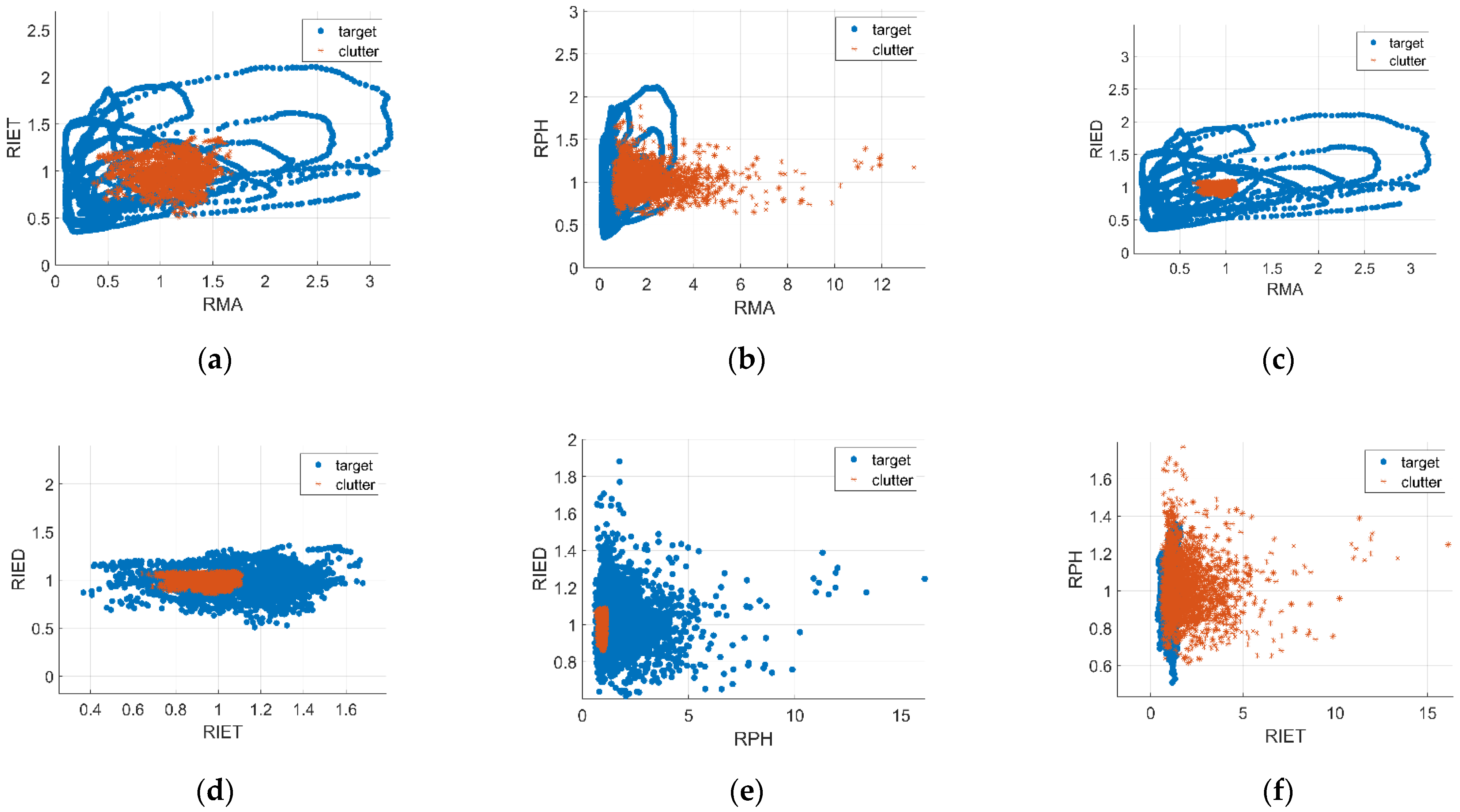
Let RMA be m i , 1 , RIET be m i , 2 , RPH be m i , 3 , RIED be m i , 4 , NCR be m i , 5 , MSC be m i , 6 , store the extracted features into the feature vector M i and get the 6-D feature vector M i = [ m i , 1 , m i , 2 , m i , 3 , m i , 4 , m i , 5 , m i , 6 ] . The eigenvector label corresponding to the target echo is 1, and the eigenvector label corresponding to the clutter is 0. Since NCR and MSC are obviously distinguishable, the feature separability analysis of NCR and MSC is not done here. Now draw the distribution of features in one-dimensional, two-dimensional, and three-dimensional space, as shown in Figure 10, Figure 11 and Figure 12. It can be clearly seen that in the one-dimensional and two-dimensional space of the feature, the feature between the target and the clutter cannot be effectively distinguished with a higher dimension of feature space, the feature of separability enhancement. In the three-dimensional space of the feature, the target and clutter can be roughly distinguished, but there are still a small number of features that are aliasing together and cannot be distinguished. Therefore, the dimension of the feature space needs to be further improved. The target and clutter can be better distinguished in the six-dimensional feature space.
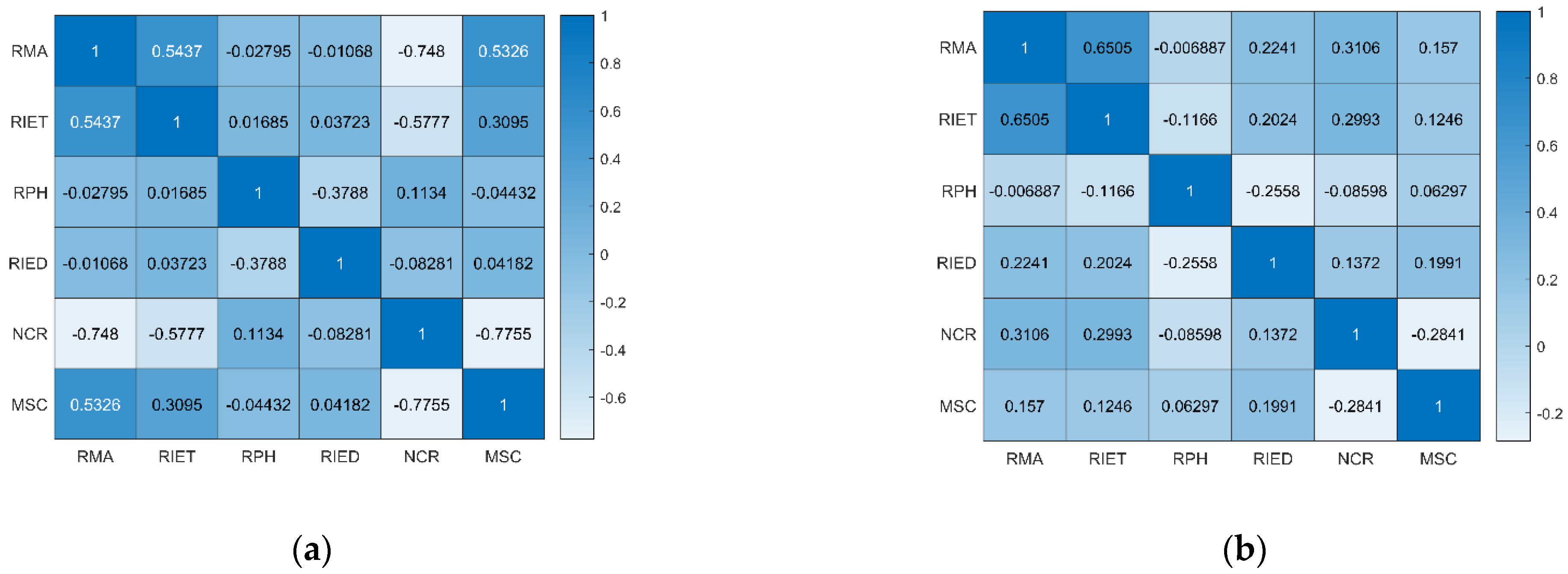
After confirming the separability between the features, Pearson’s correlation coefficient matrix is used to measure the correlation between the six standardized features and further determine whether there is a problem of feature redundancy. According to the correlation heat map Figure 13, it can be seen that there is no obvious multicollinearity problem between the features, so the six features selected are not redundant and can be used.

2.3. False-Alarm Rate Controllable Deep Forest Method

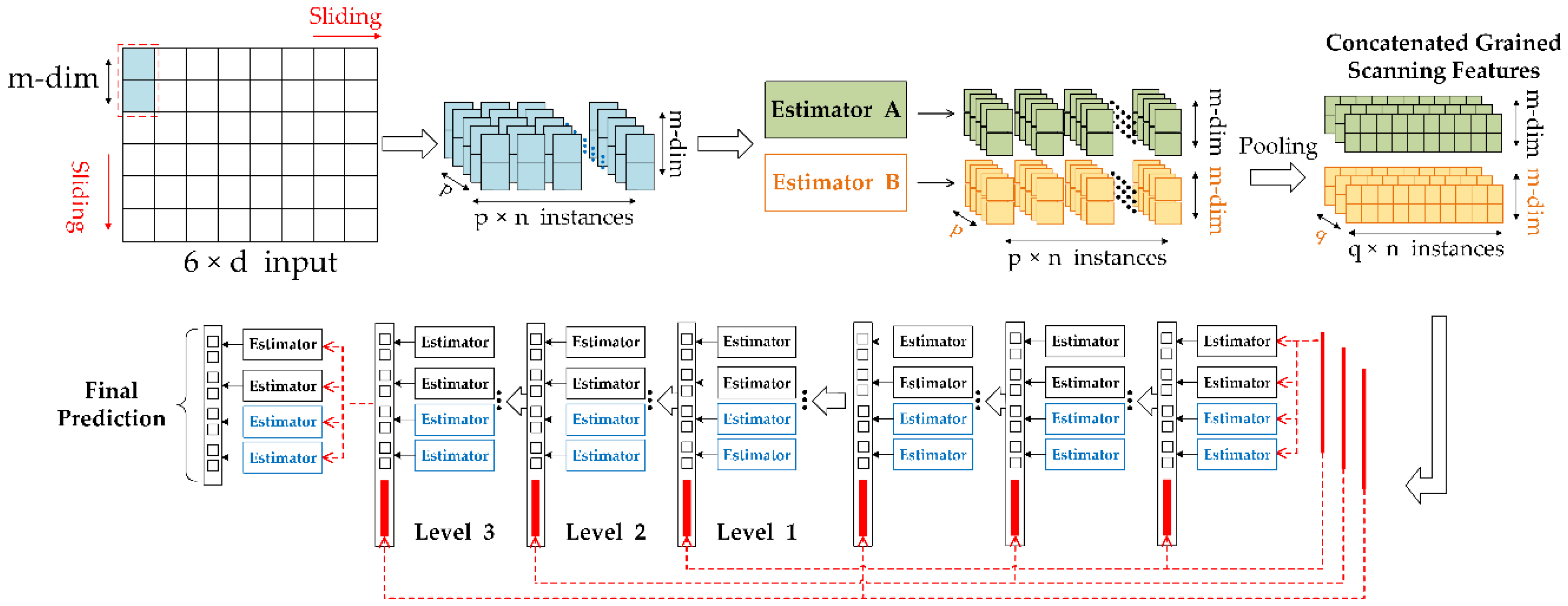
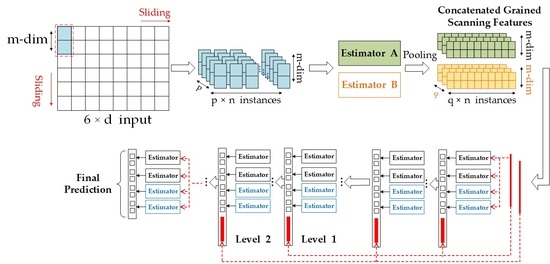
In this part, we propose a false-alarm rate (FAR) controllable detector to make the utmost use of the aforementioned features that constitute the feature space. Due to the clutter in the data set accounts for a relatively large proportion, while the target echo accounts for a relatively small proportion, so there is a problem of unbalanced categories. Algorithms, such as logistic regression and neural networks, use backpropagation to optimize parameters. The type with a small number will have less influence when backpropagating the gradient. They naturally focus more on the fit of most classes. After all, the classification of most classes is correct or not, which will affect the final overall loss. Therefore, these models are more sensitive to the uneven distribution of samples. The update strategy adopted by the tree model is completely different. Its optimization goal is to maximize the information gain after the fork. In order to do this, the tree model naturally expects the sample at each node to be purer after the fork, thus increasing the gain. In this case, even if the sample is biased, the model will pay enough attention to this category so that the impact of sample bias is greatly reduced. The tree classifier-based model, such as deep forest, is more advantageous for this kind of problem. Therefore, this paper proposes a FAR controllable detector based on deep forest [37], which is a new type of non-NN deep learning method. The structure of the deep forest model used in this article is shown in Figure 14.
Suppose that the previous processing divides the signal into d sub-signals the 6-dimensional features extracted from these sub-signals are combined to form a feature matrix that is imported into the multi-grained scanning layer in gcForest. The one-dimensional sliding pane with length m is used to re-extract the feature with step size 1, get p × n first-stage characteristics of m-dimensional. Input these first-stage characteristics into estimator A and estimator B. After training, p × n m-dimensional second-stage features can be obtained, and the q × n m-dimensional final-stage features can be acquired through a pooling layer containing a one-dimensional pooling pane of length a . Finally, the decision results can be obtained by bringing the final stage features into cascade for classification. A detailed explanation of the deep forest can be found in these two articles [37,38].
After the target detection is converted into a binary classification problem that distinguishes clutter and target, the confusion matrix can be used to measure the performance of the model applied to the binary classification problem. As shown in Table 3, the combination of results can be divided into the following four cases according to their true categories and the prediction categories of gcForest: true target (TT), false clutter (FC), false target (FT), and true clutter (TC). TT, FC, FT, and TC represent the number of samples corresponding to the cases, respectively, and the total number of samples is T T + F C + F T + T C .
In the radar system, signal detection is carried out in the interference background. There is not only system noise but also the echo reflected by the waves for the detection of weak targets on the sea surface. The interference of these noises will cause changes in decision probability. In the target signal detection of the system, the most concerned is the probability of the wrong decision, that is, the change of FAR. In model training, the preset training stop conditions are changed, and the step control of gcForest depth is added so as to obtain the optimal FAR with the minimum training time consumption. FAR how much of the clutter is misidentified as a target, its calculation formula P f can be obtained from Table 3. The ideal FAR is set as P E - f a , and the error threshold between the ideal FAR and training result is set as ξ . The pseudo-code is shown in the following Table 4.

3. Results

In this section, IPIX datasets introduced in 2.1 are used to evaluate the effect of the model and features, the experimental results of the proposed detector are also reported. In this paper, the hardware environment is a computer equipping an Intel Core I7-10700T CPU of 2.00 GHz with a 64-bit operating system and 32 GB of internal storage.
As mentioned at the beginning of 2.2, in order to obtain more features from the echo, the signals are divided into M segments of equal length d x s u b = x ( w * ( m 1 ) + 1 : w * ( m 1 ) + d ) , where m = 1 , 2 , , M and w is the overlap constant. The signal is divided into sub-segments of different lengths for feature and model evaluation. Different d corresponds to different observation times; the value of d is 512, 1024, 2048 and 4096, and the value of overlap constant w is 64. Therefore, the echo signal of each range cell can be separated into 2040, 2032, 2016, and 1984 sub-segments. In the experiment, the training set and test set are randomly selected at a ratio of 2:1 from the obtained slice data. The optimal parameters of the detection framework and the results of experiments are stated in this section, and the performance discussions are in Section 4.

3.1. Performance Analysis of Detection Framework

After a series of experiments, analyze the performance of each module and its parameters on the data, the optimal gcForest model parameters are shown in Table 5.
It should be noted that, according to the performance of the classifier in the multi-grained scanning layer, the sizes of the sliding panes used by different classifiers are not the same. Among them, the sliding pane sizes used by ExtraTreesClassifier are 5 and 6, the size used by RandomForestClassifier are 4, 5, and 6, the size used by LogisticRegression is 5.

3.2. Average Detection Probability of Different Conditions

The experiment uses the detection probability as the criterion of the result. The calculation method of the detection probability is shown in Equation (26), which represents FAR from another perspective.
P d = T T T T + F T × 100 % .
Table 6 shows the average P d of different observation times and different polarization modes. It can be seen that the dataset composed of long observation time can obtain higher detection probability, and cross-polarization mode data are more conducive to target detection. In the copolarization data, the detection result of HH polarization is better than VV polarization.

4. Discussion

This chapter uses the IPIX data [40] described in Section 2.1 to discuss the influence of detector parameter selection and data characteristics on the final detection results. In addition, the detection results of this detector are compared with the existing detectors in these documents [26,32,33,34,35,36,39].

4.1. Performance Analysis of Detection Framework

The feature vectors describe in Section 2.2 are extracted from the sub-signal and sent to the detector for training. The main parameters involved in the detector are listed in the following table. Next, the influence of parameter selection on the experimental results will be analyzed. The data used in the analysis in this part are HV polarization mode with a sub-signal length of 4096. Table 7 shows the key parameters in the model.
GcForest is an ensemble model. In principle, the based estimator used in it can be any type of classifier. First, according to the error-ambiguity decomposition [52], the principle of individual classifier selection in the ensemble-learning model is that the more accurate the individual classifier is, the more kinds of classifiers are, the better performance of the ensemble model will be [37]. Therefore, in order to obtain better training results in gcForest, in addition to improving the training accuracy of individual classifiers, it is also necessary to enhance its diversity. In practice, randomness is often added in the training process by sampling input data, using different parameters for different individual learners and other methods to enhance diversity [37]. Therefore, in the multi-grained scanning stage, three estimators with better performance are selected, ExtraTreesClassifier, RandomForestClassifier and LogisticRegression. Among them, ExtraTreesClassifier is a completely random tree model, RandomForestClassifier is a random tree model, which satisfies the basic structure of the deep forest, and LogisticRegression is the choice after comprehensive consideration of increasing model diversity and training results. In the cascade stage, two estimators XGBClassifier and SGDClassifier, are added to the selection of the previous stage, further improving the diversity of classifier selection and choosing different parameters for different models, adding changes from parameters.

4.1.1. Multi-Grained Scanning Layer

It can be found from [37] that the accuracy and the estimator number in the multi-grained scanning stage have a direct impact on the training accuracy of the subsequent cascade layer.
First, analyze the impact of the sliding pane on the accuracy of this layer. The different size panes correspond to the number of features simultaneously input to the classifier, that is, the feature diversity in the network. The experiment tests the effect of different sliding pane sizes on the results of three estimators, ExtraTreesClassifier, RandomForestClassifier and LogisticRegression, in the multi-grained scanning stage. Table 8 shows the influence of the sliding panes’ size. As the length of the sliding pane increases, the classification effect of this layer is significantly improved. Due to the characteristics of the random forest itself, it has good noise immunity, so its performance is significantly better than the other two classifiers, even if the size of the sliding panes is small.
Next, analyze the impact of the different number of classifier combinations using different sliding panes on the result in the cascade layer. The sliding pane sizes with good results in the previous experiment are selected to match with the estimators, and the performance in the cascade layer after obtaining multi-grained features and time cost in the multi-grained scanning stage are tested. Figure 15 shows the results with a composite chart composed of a histogram representing accuracy and a line chart representing time consumption. When only one classifier, RandomForestClassifier, exists at this stage, although the three-parameter values of the classifier with the best results were selected, its performance is still the worst compared to the other two combinations. The combination with the largest number of classifiers and the largest types of parameters obtained the best results, with an accuracy rate of 99.63% for the training set and 99.66% for the test set. Its time-consuming is also the shortest, only 655 s. It is not difficult to see that considering the training efficiency, increasing the number and types of classifiers used within a reasonable range will have a positive effect on the results. This is also in line with the law of the influence of the accuracy and diversity of the individual classifiers of ensemble-learning on the results of the ensemble model.
After a series of experiments and analysis, it is finally decided to use the multi-grained scanning layer with two ExtraTreesClassifiers with pane size 5 and 6, three RandomForestClassifiers with pane size 4, 5, and 6, one LogisticRegression with pane size 6 for the preliminary training of features.

4.1.2. Cascade Layer

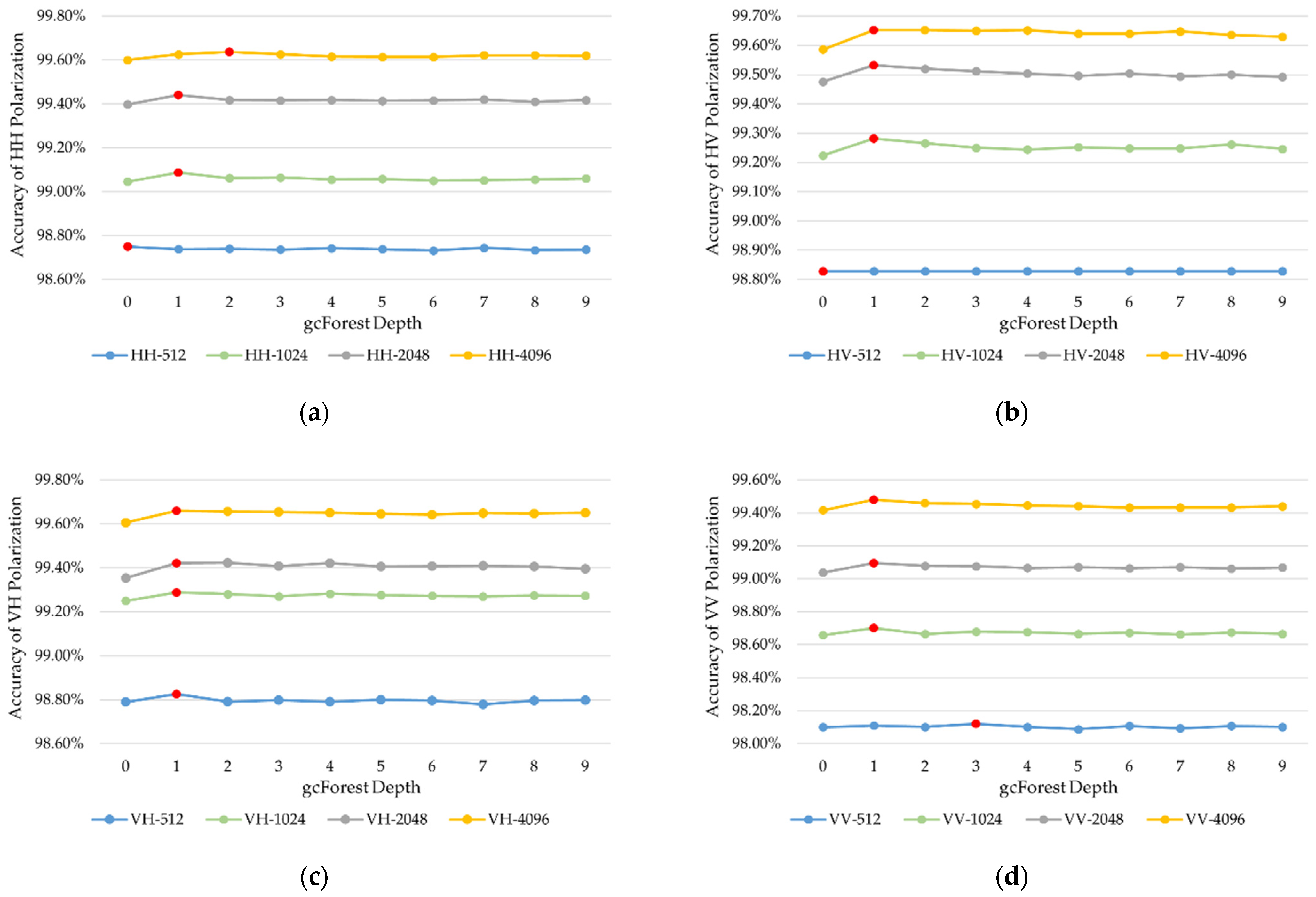
In the cascade layer, one of the keys to ensuring training accuracy is to keep the diversity of classifiers. Therefore, this paper chooses five classifiers RandomForestClassifier, ExtraTreesClassifier, XGBClassifier, SGDClassifier, LogisticRegression, as the classifiers in the cascade stage. From the experiment, it is found that the depth of gcForest affects the change of detection probability. It can be seen from Figure 16 that detection probability increases first and then decreases with the growth of training depth in most cases.
In order to obtain the optimal accuracy and highest training efficiency, a false alarm controllable detector is designed by controlling the depth of the cascade layer in gcForest. Combined with the pre-analysis of the data, the initial depth is set as six, and the step length is set as 2. When P E - f a has reached the expected value within the allowable range of error threshold before the preset depth, the corresponding optimal detection probability is taken as the output result, and the model at this time is saved. If P E - f a it fails to reach the expected value before the maximum depth, the best detection probability during the training is output, and the corresponding training model is saved. The expected FAR P E - f a is set as 0.01, and the error threshold ξ is set as 0.001 in these experiments. Table 9 is the average FAR of the detector with different observation times and different polarization modes.
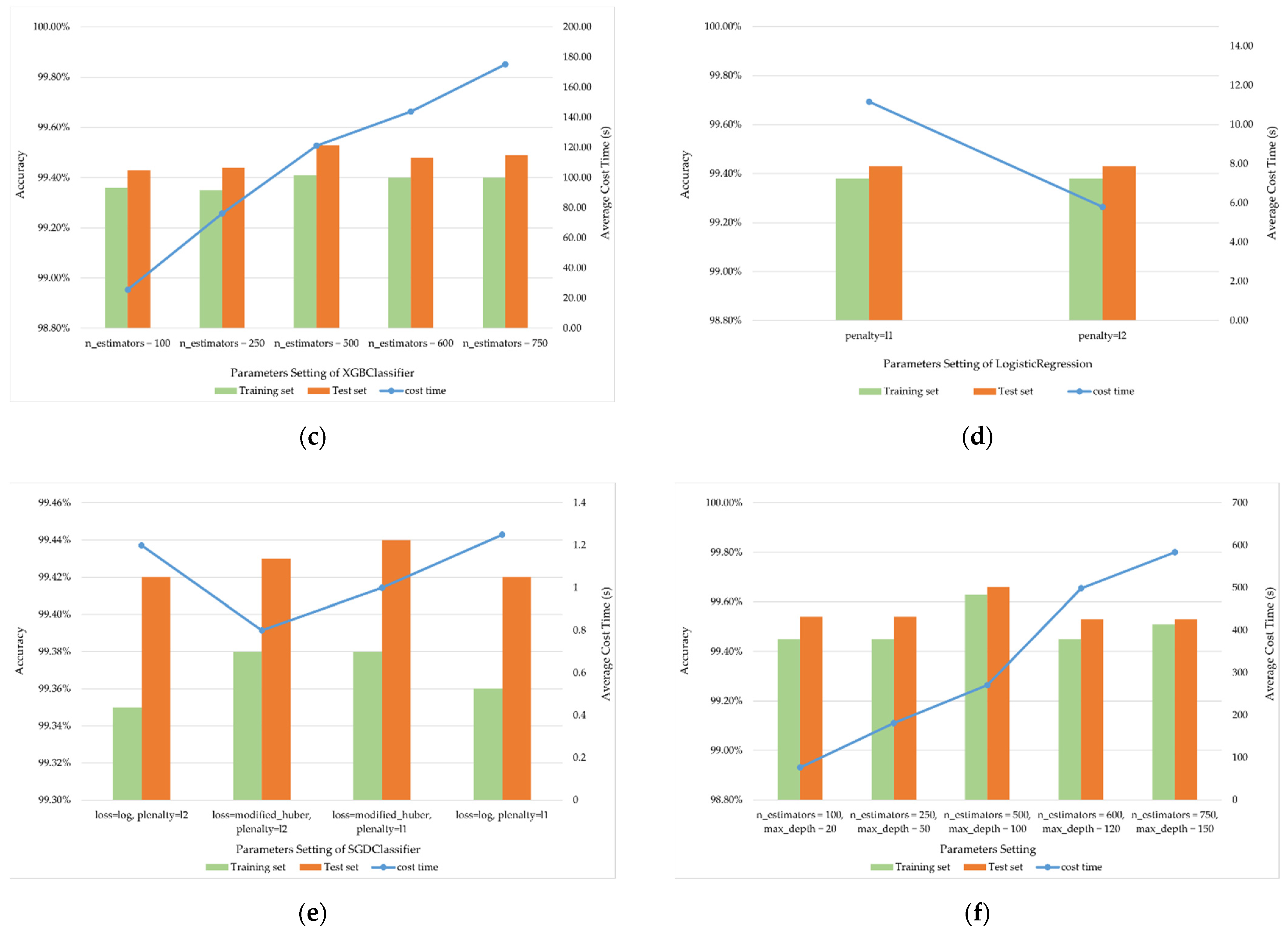
In addition, the effect of parameter settings and complexity on the performance of the cascade stage is also discussed. The experiment separately discusses the five models used in the cascade stage and adjusts the different parameters involved to explore the impact of their parameters and complexity on performance. The parameters adjusted in the experiment are shown in the following Table 10.
Among them, for ExtraTreesClassifier, RandomForestClassifier, and XGBClassifier, the parameters named n_estimators and max_depth affect the amount of calculation in the training process so they have a greater impact on the time cost. Using n_estimators = 500 and max_depth = 100 as benchmarks, zoom in or zoom out the values of these two parameters proportionally and observe their impact on accuracy and training time. For LogisticRegression and SGDClassifier, the commonly used parameter penalty represents the choice of regularization term, and the parameter loss in SGDClassifier represents the choice of the loss function.
The combined Figure 17a–e respectively represents the impact on the performance of the parameters in the several above classifiers according to Table 10. Figure 17f shows the effect of changing the values of n_estimators and max_depth in ExtraTreesClassifier and RandomForestClassifier after combining several classifiers and the value of n_estimators in XGBClassifier on the final model. At this time, LogisticRegression and SGDClassifier use the parameters that can achieve the best results in the previous experiments. In Figure 17, the histogram represents the accuracy of the detector for the training set and test set, and the line graph represents the average training time of each layer.
It can be seen from this that Figure 17a–c illustrates that the number of estimators in the classifiers and the classifiers’ max depth grows within a certain range. Although the training time is raising, the accuracy of the model has been improved. However, when the number and depth increase to a certain level, the accuracy of the model decreases slightly, but the training time increases significantly. Figure 17d,e illustrates that the appropriate selection of loss function and regularization term will improve the accuracy of training and greatly shorten the training time of each layer. Figure 17f shows that ensemble-learning can improve training accuracy to a certain extent, and the selection of appropriate parameters will bring higher accuracy and more cost-effective time consumption.

4.2. Performance Analysis of Data

This part will analyze from two perspectives of data characteristics and the feature selects in this experiment. IPIX dataset is radar echo data with four polarization modes. In order to obtain more information from the limited data, the original data are decomposed into different lengths in the experiment, corresponding to different observation times. Therefore, signals with different polarization and different lengths are trained to analyze their influence on target detection, and the influence of individual features on detection is discussed in the second part.

4.2.1. Influence of Polarization and Observation Length

Table 11 shows the details of the average detection probability in different observation times and different polarization modes. As the observation time accumulates, the detector’s ability to distinguish the target becomes stronger. Observation time increased by eight times, and the average detection probability decreases 0.97%. Due to the copolarization is extremely sensitive to changes in sea clutter, and changes in sea conditions will have a great impact on the SCR. Therefore, its noise immunity is not as good as cross-polarization, so the probability of using cross-polarization to detect targets is higher. In different polarization modes, the average detection probability of HV polarization is 0.47% lower than that of VV polarization.

4.2.2. Feature Importance

A feature is randomly removed to determine the impact of the test feature on the detection performance. Table 12 lists the performance loss of different features by using the data with a sub-signal length of 4096 in training and testing different polarization data. The rest of the information about the data is the same as before. It can be found that VV polarization is sensitive to characteristic changes. RPH, RIED, and MSC have a greater impact on the detection results, and any removal of a feature will have a negative impact on the detection results, which can indicate that each feature contributes to the detection results, so it is necessary and effective to construct a joint feature space.

4.3. The Comparision of Results of Different Methods

In this subsection, the validity of the model is verified from different angles. First, several deep learning and ensemble-learning models are selected to verify the effectiveness of the proposed method’s model selection and feature vector construction. Then, the detection results of the proposed model are compared with that of the published detectors.

4.3.1. Model Validity Check

In order to verify the effectiveness of the model and the construction of feature vectors, this paper selects representative methods in the deep learning model and the ensemble-learning model, respectively and inputs the feature vectors constructed in this paper into the network for classification. These comparison methods are multilayer perceptron classifier, SVM (linear classifier), logistic regression, k-nearest neighbors, Gaussian naïve Bayes and Xgboost. The selection of the SVM kernel function is briefly explained here. The kernel function used in SVM can be divided into Linear kernel and Gaussian kernel, which is what we often call linear kernel and RBF kernel. The choice of the two will be different due to the different problems they deal with, the number of features and samples. The sample data in this experiment is large, and the number of features is small. The calculation uses the libSVM library developed by National Taiwan University. The library’s guidance document states that when the sample size is greater than 10,000, RBF will bring huge time consumption, so Linear kernel support vector machines are more suitable for this situation.
In the experiments, take the polarization model as HV, d = 4096 and the observation time for one decision is 4.096 s. The classification results are shown in Table 13.
It can be seen from the experiment results that, first, the selection of features is suitable for the classification of targets and clutter, and second, the performance of the proposed detector is the best among all models.

4.3.2. Comparison of Detection Performance

Next, on the 14 IPIX datasets, the six-feature fusion deep forest-based detector proposed in this paper is compared with the three-feature detector using SVM-based [33] and Decision Tree-based [34] as the detection framework. Figure 18 shows the accuracy performance of the three classifiers for the target and clutter classification under the four polarization modes of 14 data. The observation time of the data selection is 4.096 s. It can be seen from the results that in the four polarization modes, the performance of the SVM-based detector is slightly inferior to the other two methods. Its average detection accuracy rate is 88.87%, average FAR is 0.0319. From Figure 17, the performance of the SVM-based detector is not very stable, and there will be large fluctuations in different data, indicating that the changes in sea clutter and target echo caused by changes in sea conditions have a greater impact on the detector. Another problem with this model is that the classification accuracy of the target is extremely low in some data, but the classification of clutter is fully accurate. The main reason for this is that clutter data accounts for a large proportion, and even though SVM is a more suitable model for dealing with class imbalance problems, it does not perform very well in handling this problem. The average detection accuracy rate of a decision tree-based detector is 96.26%, the average FAR is 0.0190, the test results are maintained at a relatively good level. Experiments show that the anti-interference of the tree model is more robust.
Deep forest-based detector’s average detection accuracy rate is 98.76%; the average FAR is 0.0080. The performance of this model is the best in terms of the stability of its detection accuracy in each data or its achieved FAR. The results show that a combination of six-dimensional features and the deep forest-based detector has strong anti-interference performance in changing environments. The classification accuracy of the detector for clutter and target is extremely high. Therefore, the effect of the ensemble-learning method in category imbalance samples is also verified.
Table 14 shows the evaluation of the performance between the proposed detector in this article with the other six methods under varying detection situations. They are fractal-based detector [26], tri-feature-based detector [32], TF-tri-feature-based detector [36], feature-compression-based detector [39], decision tree-based detector [34] and K-NN FAR-controlled Detector [35]. Due to the different number and types of features used and different detection frameworks, the performance of the final constituent detectors are also different.
From the results that the fractal-based detector obtains a lower detection accuracy rate because it only uses a fractal feature. The tri-feature-based detector, TF-tri-feature-based detector and decision tree-based detector use three types of features to form 3-D feature vectors. Both tri-feature-based detectors, TF-tri-feature-based detectors use a detector based on the improved convex-hull learning algorithm to detect the target and the decision tree-based detector chooses an improved decision tree as the detection framework. The results show that the tri-feature-based detector and TF-tri-feature-based detector have higher detection accuracy than fractal-based detector, which uses only one feature. The addition of features helps to improve the target detection accuracy.
While decision tree-based detector, which also uses 3-D features, has a stronger detection ability than the tri-feature-based detector and TF-tri-feature-based detector, indicating that an appropriate framework can effectively improve the detection ability of weak targets. Feature-compression-based detector and K-NN FAR-controlled detector use the same features to form the 7-D feature vectors. The difference is that the feature-compression-based detector compaction the 7-D feature vectors to 3-D and uses the optimized convex-hull learning algorithm to identify the target and clutter, while K-NN FAR-controlled detector directly takes the extracted 7-D feature vectors as input and uses the improved KNN algorithm for detection. The comparison of the two results shows that using the same features; the machine learning framework can bring better learning results and higher detection accuracy. It can be found by the comparison; the proposed detector can provide the best detection results under the four polarization modes and different observation time length conditions.
The proposed method is compared with the optimal K-NN FAR-control detector, when FAR = 0.01 and the observation time is 0.512 s, and 1.024 s, the average detection accuracy of K-NN FAR-controlled detector is 85.00% and 89.23%, and that of the proposed method is 98.65% and 99.10%, respectively 13.65% and 9.87% higher. This fully proves that the constructed feature vector has better robustness and anti-interference, and the proposed detector is more effective.
Aiming at the current problem of weak target detection on the sea surface, one can start to solve this problem from multiple perspectives, such as exploring effective features to construct robust feature vectors and constructing a reasonable detection framework to maximize the utilization of feature vectors.

5. Conclusions

The detection of floating small targets under the background of sea clutter is a recognized problem and has attracted extensive attention. With the stealth and miniaturization of sea targets, improving the detection ability to float small targets is of great significance for sea target detection. This paper proposes a high-dimensional feature space detection method based on deep learning methods and obtains satisfactory results. The specific contributions made are summarized as follows:
  • Six features are selected from three domains to construct feature vectors for detection. Ocean conditions are complex and constantly changing; a single feature cannot effectively detect weak targets on the sea surface. In order to obtain efficient and accurate detection results, this paper extracts six features that can distinguish weak targets and clutter from the time domain, frequency domain, and time–frequency domain, namely RMA, RIET, RPH, RIED, NCR and MSC;
  • The deep forest model is used as the weak target detection framework for the first time, and the main algorithm used is gcForest. The model is improved by introducing the expected FAR value into the stop growth judgment condition of the gcForest cascade level to construct a FAR controllable model.
The target detection is transformed into a binary classification problem of clutter and target. Experiments verify the effectiveness of the model and compare the results with the proposed method’s results; the model performance reaches the state of the art.
At the end of this paper, the limitation and development of weak target detection at sea level are briefly explained. The lack of publicly marked measurement data for weak targets at the sea surface is the biggest limitation of the current problem. In addition to IPIX data, there is a CSIR dataset jointly owned by ARMSCOR and SAAF, but unfortunately, this dataset is no longer available to the public. Although the data provided by the Naval Aviation University of China [53] is publicly downloaded, it is not very suitable for the training of weak target detection due to the lack of information on cooperative targets. There are many other datasets, but they are not public. A large amount of measured data are helpful to construct a data set with a balance of positive and negative samples, which is also helpful to further reduce FAR and improve detection rate. Therefore, constructing a complete annotated dataset is a long-term task.
The existing detectors still have plenty of room for development. To further improve the performance of the detector, the future development direction of feature-based detectors can mine more representative features from different domains and improve the detection performance of the detection framework in a shorter observation time. At the same time, with the target constantly updating iteration, the detection of targets with smaller size and stealth materials is also worthy of attention. Combining the intelligence of emerging disciplines with feature-based detection methods can more effectively detect targets and improve the detection performance of slow, floating small targets under the background of sea clutter.

Author Contributions

Methodology, J.Z.; software, J.Z., validation, J.Z.; investigation, J.Z.; resources, H.S.; writing—original draft preparation, J.Z.; writing—review and editing, J.Z.; visualization, J.Z.; supervision, H.S.; project administration, H.S.; funding acquisition, H.S. All authors have read and agreed to the published version of the manuscript.

Funding

This work is supported by the foundation item of the National Key R&D Program of China (Y7BD160194).

Institutional Review Board Statement

Not applicable.

Informed Consent Statement

Not applicable.

Data Availability Statement

The article usage data is available on the website: http://soma.ece.mcmaster.ca/ipix/dartmouth/index.html (accessed on 2 February 2021).

Acknowledgments

The authors would like to thank all reviewers and editors for their comments on this paper.

Conflicts of Interest

The authors declare no conflict of interest.

References

  1. Peng-Lang, S.; Bao, Z.; Su, H. Nonparametric detection of FM signals using time-frequency ridge energy. IEEE Trans. Signal Process. 2008, 56, 1749–1760. [Google Scholar] [CrossRef]
  2. Xiaolong, C.; Jian, G.; Yong, H.; You, H. Radar low-observable target detection. Sci. Technol. Rev. 2017, 35, 30–38. [Google Scholar]
  3. You, H.; Yong, H.; Jian, G.; Chen, X. An overview on radar target detection in sea clutter. Mod. Radar. 2014, 36, 1–9. [Google Scholar]
  4. Yufang, T. Research on Weak Target Detection in Sea Clutter. Ph.D. Thesis, Ocean University of China, Qingdao, China, 2013. [Google Scholar]
  5. Chen, Y.; Li, Y.; Wang, J.; Chen, W.; Zhang, X. Remote Sensing Image Ship Detection under Complex Sea Conditions Based on Deep Semantic Segmentation. Remote Sens. 2020, 12, 625. [Google Scholar] [CrossRef] [Green Version]
  6. Dongchen, L. A feature Detection Method for Small Targets in Sea Clutter. Ph.D. Thesis, Xidian University, Xi’an, China, 2013. [Google Scholar]
  7. Liu, G.; Zhang, X.; Meng, J. A Small Ship Target Detection Method Based on Polarimetric SAR. Remote Sens. 2019, 11, 2938. [Google Scholar] [CrossRef] [Green Version]
  8. Joshi, S.K.; Baumgartner, S.V.; da Silva, A.B.C.; Krieger, G. Range-Doppler Based CFAR Ship Detection with Automatic Training Data Selection. Remote Sens. 2019, 11, 1270. [Google Scholar] [CrossRef] [Green Version]
  9. Xu, S.; Bai, X.; Guo, Z.; Shui, P. Status and prospects of feature-based detection methods for floating targets on the sea surface. J. Radars 2020, 9, 684–714. [Google Scholar] [CrossRef]
  10. Dugundji, J.; Ackerlind, E. Automatic bias control for a threshold detector. IRE Trans. Inf. Theory 1957, 3, 65–70. [Google Scholar] [CrossRef]
  11. Endresen, K.; Hedemark, R. Coincidence techniques for radar receivers employing a double-threshold method of detection. Proc. IRE 1961, 49, 1561–1567. [Google Scholar] [CrossRef]
  12. Watts, S. Cell-averaging CFAR gain in spatially correlated K-distributed clutter. IEE Proc. Radar Sonar Navig. 1996, 143, 321–327. [Google Scholar] [CrossRef]
  13. Steenson, B.O. Detection performance of a mean-level threshold. IEEE Trans. Aerosp. Electron. Syst. 1968, 4, 529–534. [Google Scholar] [CrossRef]
  14. Conte, E.; Longo, M.; Lops, M. Performance analysis of CA-CFAR in the presence of compound Gaussian clutter. Electron. Lett. 1988, 24, 782–783. [Google Scholar] [CrossRef]
  15. Hansen, V.G. Constant false alarm rate processing in search radars. In Proceedings of the IEEE 1973 International Radar Conference, London, UK, 23–25 October 1973; pp. 325–332. [Google Scholar]
  16. Weiss, M. Analysis of some modified cell-averaging CFAR processors in multiple-target situations. IEEE Trans. Aerosp. Electron. Syst. 1982, 1, 102–114. [Google Scholar] [CrossRef]
  17. Trunk, G.V. Range resolution of targets using automatic detectors. IEEE Trans. Aerosp. Electron. Syst. 1978, 5, 750–755. [Google Scholar] [CrossRef]
  18. Rohling, H. Radar CFAR thresholding in clutter and multiple target situations. IEEE Trans. Aerosp. Electron. Syst. 1983, 4, 608–621. [Google Scholar] [CrossRef]
  19. Rohling, H. New CFAR-processor based on an ordered statistic. In Proceedings of the International Radar Conference, Arlington, VA, USA, 6–9 May 1985; pp. 271–275. [Google Scholar]
  20. Kelly, E.J. An adaptive detection algorithm. IEEE Trans. Aerosp. Electron. Syst. 1986, 2, 115–127. [Google Scholar] [CrossRef] [Green Version]
  21. Fuhrmann, D.R.; Kelly, E.J.; Nitzberg, R. A CFAR adaptive matched filter detector. IEEE Trans. Aerosp. Electron. Syst. 1992, 28, 208–216. [Google Scholar]
  22. Conte, E.; Lops, M.; Ricci, G. Asymptotically optimum radar detection in compound-Gaussian clutter. IEEE Trans. Aerosp. Electron. Syst. 1995, 31, 617–625. [Google Scholar] [CrossRef] [Green Version]
  23. Richmond, C.D. Analysis of an adaptive detection algorithm for non-homogeneous environments. In Proceedings of the 1998 23rd IEEE International Conference on Acoustics, Speech and Signal Processing, ICASSP 1998, Seattle, WA, USA, 12–15 May 1998. [Google Scholar]
  24. Lo, T.; Leung, H.; Litva, J.; Haykin, S. Fractal characterisation of sea-scattered signals and detection of sea-surface targets. In IEEE Proceedings F (Radar and Signal Processing); IET Digital Library: New York, NY, USA, 1993; Volume 140. [Google Scholar]
  25. Hu, J.; Tung, W.W.; Gao, J.B. Detection of low observable targets with sea clutter by structure function based multifractal analysis. IEEE Trans. Antennas Propag. 2006, 54, 136–143. [Google Scholar] [CrossRef]
  26. Xu, X.-K. Low observable targets detection by joint fractal properties of sea clutter: An experimental study of IPIX OHGR datasets. IEEE Trans. Antennas Propag. 2010, 58, 1425–1429. [Google Scholar]
  27. Jian, G.; Ning-bo, L.; Jian, Z.; Jie, S. Multifractal Correlation Characteristic of Real Sea Clutter and Low-Observable Targets Detection. J. Electron. Inf. Technol. 2010, 32, 54–61. [Google Scholar] [CrossRef]
  28. Fan, Y.; Luo, F.; Li, M.; Hu, C.; Chen, S. The Multifractal Properties of AR Spectrum and Weak Target Detection in Sea Clutter Background. J. Electron. Inf. Technol. 2016, 38, 455–463. [Google Scholar] [CrossRef]
  29. Guan, J.; Liu, N.B.; Huang, Y.; He, Y. Fractal characteristic in frequency domain for target detection within sea clutter. IET Radar Sonar Navig. 2012, 6, 293–306. [Google Scholar] [CrossRef]
  30. Chen, X.L.; Guan, J.; He, Y.; Zhang, J. Detection of low observable moving target in sea clutter via fractal characteristics in fractional Fourier transform domain. IET Radar Sonar Navig. 2013, 7, 635–651. [Google Scholar] [CrossRef]
  31. Wang, X.; Liu, J.; Liu, H. Small target detection in sea clutter based on Doppler spectrum features. In Proceedings of the 2006 CIE International Conference on Radar, Shanghai, China, 16–19 October 2006; pp. 1–4. [Google Scholar]
  32. Shui, P.-L.; Li, D.; Xu, S. Tri-feature-based detection of floating small targets in sea clutter. IEEE Trans. Aerosp. Electron. Syst. 2014, 50, 1416–1430. [Google Scholar] [CrossRef]
  33. Li, Y.; Xie, P.; Tang, Z.; Jiang, T.; Qi, P. SVM-based sea-surface small target detection: A false-alarm-rate-controllable approach. IEEE Geosci. Remote Sens. Lett. 2019, 16, 1225–1229. [Google Scholar] [CrossRef] [Green Version]
  34. Zhou, H.; Tao, J. Decision tree based sea-surface weak target detection with false alarm rate controllable. IEEE Signal Process. Lett. 2019, 26, 793–797. [Google Scholar] [CrossRef]
  35. Guo, Z.; Shui, P.; Bai, X.; Xu, S.; Li, D. Sea-Surface small target detection based on K-NN with controlled false alarm rate in sea clutter. J. Radars 2020, 9, 654–663. [Google Scholar] [CrossRef]
  36. Shi, S.-N.; Shui, P.-L. Sea-surface floating small target detection by one-class classifier in time-frequency feature space. IEEE Trans. Geosci. Remote Sens. 2018, 56, 6395–6411. [Google Scholar] [CrossRef]
  37. Zhou, A.-H.; Feng, J. Deep forest: Towards an alternative to deep neural networks. In Proceedings of the 26th International Joint Conference on Artificial Intelligence (IJCAI’17), Melbourne, Australia, 19–25 August 2017; pp. 3553–3559. [Google Scholar]
  38. Zhang, J.; Song, H.; Zhou, B. SAR Target Classification Based on Deep Forest Model. Remote Sens. 2020, 12, 128. [Google Scholar] [CrossRef] [Green Version]
  39. Shui, P.; Guo, Z.; Shi, S. Feature-Compression-Based Detection of Sea-Surface Small Targets. IEEE Access 2019, 8, 8371–8385. [Google Scholar] [CrossRef]
  40. The Dartmouth Database [DB/OL]. Available online: http://soma.ece.mcmaster.ca/ipix/dartmouth/index.html (accessed on 10 November 2020).
  41. Maps and Pictures of the IPIX Radar at OHGR/Dartmouth [DB/OL]. Available online: http://soma.ece.mcmaster.ca/ipix/dartmouth/ohgrmaps.html (accessed on 10 November 2020).
  42. Wind, Waves, Weather during Data Collection at OHGR/Dartmouth [DB/OL]. Available online: http://soma.ece.mcmaster.ca/ipix/dartmouth/windwave.html (accessed on 10 November 2020).
  43. Guo, L.; Cheyoung, K. Light-scattering models for a spherical particle above a slightly dielectric rough surface. Microw. Opt. Technol. Lett. 2002, 33, 142–146. [Google Scholar]
  44. Guo, L.; Wang, Y.; Wu, Z. Research on Backward Compound Electromagnetic Scattering and Doppler Spectrum of Dynamic Sea Surface and Moving Spherical Target. Sci. China Ser. G 2008, 38, 34–45. [Google Scholar]
  45. Jia, L.; Guo, L.; Li, J. Research on Compound Electromagnetic Scattering from Sea Surface and Three-dimensional Floating Target Above Based on FDTD Method. Aero Weaponry 2015, 6, 8–13. [Google Scholar]
  46. Long, M.W. Radar reflectivity of land and sea. DCHC 1975. [Google Scholar] [CrossRef]
  47. Wang, X.S.; Yang, Y. Overview on cognition of clutter and target polarization characteristics for maritime radar. Chin. J. Radio Sci. 2019, 34, 665–6675. (In Chinese) [Google Scholar] [CrossRef]
  48. Zuo, L.; Chan, X.; Lu, X.; Li, M. A weak target detection method in sea clutter based on joint space-time-frequency decomposition. J. Radars 2019, 8, 335–343. [Google Scholar] [CrossRef]
  49. Gini, F.; Farina, A.; Montanari, M. Vector subspace detection in compound-Gaussian clutter, part II: Performance analysis. IEEE Trans. Aerosp. Electron. Syst. 2002, 38, 1312–1323. [Google Scholar] [CrossRef]
  50. Conte, E.; Farina, A.; De Maio, A. Design and analysis of a knowledge-aided radar detector for doppler processing. IEEE Trans. Aerosp. Electron. Syst. 2006, 42, 1058–1079. [Google Scholar] [CrossRef]
  51. Jeong, J.; Williams, W.J. Kernel design for reduced interference distributions. IEEE Trans. Signal Process 1992, 40, 402–412. [Google Scholar] [CrossRef]
  52. Krogh, A.; Vedelsby, J. Neural Network Ensembles, Cross Validation, and Active Learning. In International Conference on Neural Information Processing Systems; MIT Press: Cambridge, MA, USA, 1995; pp. 231–238. [Google Scholar]
  53. Liu, N.; Dong, Y.; Wang, G.; Ding, H.; He, Y. Sea-detecting X-band radar and data acquisition program. J. Radars 2019, 8, 656–667. [Google Scholar] [CrossRef]
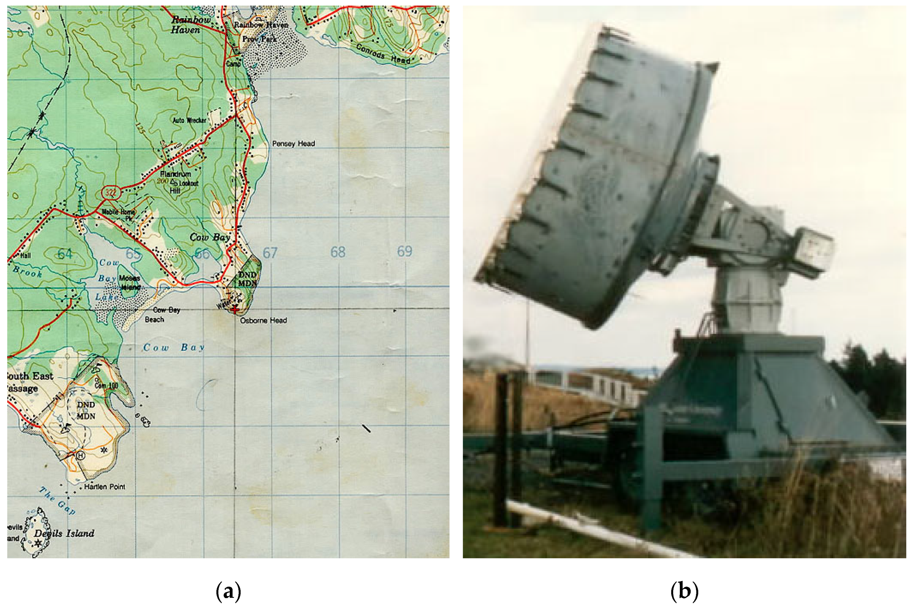
Figure 1. The collection location and a picture of the Intelligent Pixel Processing X-band (IPIX) radar. (a) Topo map of IPIX radar data collecting site in 1993, the latitude and longitude coordinates of the collection site are 44°36.72′N and 63°25.41′W, respectively; (b) IPIX radar picture.
Remotesensing 13 00812 g001
Figure 2. Average signal–clutter ratio (SCR) of 14 sets of echo data.
Remotesensing 13 00812 g002
Figure 3. Relative mean amplitude (RMA) feature of the first dataset. (a) The amplitude of primary cell where target exists and the average amplitude of clutter-only cell; (b) The histogram of RMA at the primary cell where target exists and randomly selected clutter-only cell.
Remotesensing 13 00812 g003
Figure 4. Relative information entropy in the time domain (RIET) feature of the first dataset. (a) the histogram of RIET at the primary cell where target exists and randomly selected clutter-only cell; (b) the average RIET of radar echo in each range cell.
Remotesensing 13 00812 g004
Figure 5. Frequency spectrogram of sea clutter and target signals from different echoes. (a) is the spectrogram of data names 19931107_135603_starea; (b) is the spectrogram of data names 19931111_163625_starea.
Remotesensing 13 00812 g005
Figure 6. Relative value of Doppler peak height (RPH) feature of the first dataset. (a) the histogram of RPH at the primary cell where target exists and randomly selected clutter-only cell; (b) the average RPH of radar echo in each range cell.
Remotesensing 13 00812 g006
Figure 7. RIED feature of the first dataset. (a) the histogram of RIED at the primary cell where target exists and randomly selected clutter-only cell; (b) the average RIED of radar echo in each range cell.
Remotesensing 13 00812 g007
Figure 8. Time–frequency character figures of target echo and sea clutter. (a) Choi–Williams distribution (CWD) of target echo; (b) CWD of sea clutter; (c) N-CWD(Normalized–CWD) of target echo; (d) N–CWD of sea clutter.
Remotesensing 13 00812 g008
Figure 9. Important time–frequency points (ITFP) figures of target echo and sea clutter. (a) ITFP of target echo; (b) ITFP of sea clutter.
Remotesensing 13 00812 g009
Figure 10. Representation of one-dimensional characteristics on targets and clutter. (a) RMA; (b) RIET; (c) RPH; (d) RIED.
Remotesensing 13 00812 g010
Figure 11. Representation of two-dimensional characteristics on targets and clutter. (a) RMA—RIET; (b) RMA—RPH; (c) RMA—RIED; (d) RIET—RIED; (e) RPH—RIED; (f) RIET—RPH.
Remotesensing 13 00812 g011
Figure 12. Representation of three-dimensional characteristics on targets and clutter. (a) RMA—RPH—RIET; (b) RPH—RIET—RIED; (c) RIET—RMA—RIED; (d) RPH—RMA—RIED.
Remotesensing 13 00812 g012
Figure 13. Characteristic correlation analysis of target and clutter. (a) characteristic correlation of target; (b) characteristic correlation of clutter.
Remotesensing 13 00812 g013
Figure 14. Flow diagram of deep forest.
Remotesensing 13 00812 g014
Figure 15. Cascade layer and time cost in the multi-grained scanning layer.
Remotesensing 13 00812 g015
Figure 16. The influence of gcForest on detection probability of different polarization, red points in charts are the points with the highest detection probability. (a) HH polarization; (b) HV polarization; (c) VH polarization; (d) VV polarization.
Remotesensing 13 00812 g016
Figure 17. The influence of parameters on training accuracy and time-consuming (a) performance of ExtraTreeClassifier; (b) performance of RandomForestClassifier; (c) performance of XGBClassifier; (d) performance of LogisticRegression; (e) performance of SGDClassifier; (f) performance of synthesis model.
Remotesensing 13 00812 g017aRemotesensing 13 00812 g017b
Figure 18. The influence of gcForest on detection probability of different polarization, red points in charts are the points with the highest detection probability. (a) HH polarization; (b) HV polarization; (c) VH polarization; (d) VV polarization.
Remotesensing 13 00812 g018
Table 1. Parameters of IPIX radar in 1993.
Parameter NameValue
Radar carried frequency9.39 GHz
Pulse length200 nanoseconds
PRF1000 Hz
Antenna beamwidth0.9 degrees
Antenna gain45.7 dB
Range cell(2574 2589 … nrange … 2769) meters
Azimuth angle(129.4958 129.4958 … nsweep … 129.5453) degrees
Elevation angle(359.5111 359.5111 … nsweep … 359.5111) degrees
Unambiguous velocity7.892 m/s
Range resolution30 m
Data format(nsweep × ntxpol × nrange × nadc) ADC output
nsweep131,072
ntxpol2
nrange14
nadc4
Working modeResident mode
Table 2. Description of IPIX radar data acquired in 1993.
NumberData NameTarget Cell (Primary)Target Cell (Secondary)Wave Height (m) 1Wind Speed (km/h)
119931107_135603_starea98–112.019
219931107_141630_starea98–112.019
319931107_145028_starea87–92.0113
419931108_213827_starea76–80.989
519931108_220902_starea76–81.109
619931109_191449_starea76–80.8919
719931109_202217_starea76–90.8919
819931110_001635_starea75–81.019
919931111_163625_starea87–100.6320
1019931118_023604_stareC000087–101.6910
1119931118_035737_stareC0000108–121.697
1219931118_162155_stareC000076–90.9133
1319931118_162658_stareC000076–90.9133
1419931118_174259_stareC000076–90.9128
1 Since the recording time of wave height data are scattered and not fixed, the wave height data in the table is the wave height at the time point closest to the data collection time.
Table 3. Confusion matrix of sea-surface weak target detection.
Predicted ClassSummary
TargetClutter
Actual ClassTargetTrue target (TT)False clutter (FC)Actual Target
(TT + FC)
ClutterFalse target (FT)True clutter (TC)Actual Clutter
(FT + TC)
SummaryPredicted target
(TT + FT)
Predicted clutter
(FC + TC)
TT + FT + FC + TC
Table 4. Pseudo-code of false alarm rate (FAR)-controllable deep forest model.
Algorithm: FAR-Controllable Deep Forest Model.
Input:
  Dataset: eigenvector matrix M = { M i } i = 1 W , M i is 6-dim eigenvector M i = [ m i , 1 , m i , 2 , m i , 3 , m i , 4 , m i , 5 , m i , 6 ] ;
  Label set: L = { L i } i = 1 W ;
  Expected FAR: P E - f a ;
  Error threshold: ξ ;
  Preset depth of gcForest: H ;
  Step length of depth: Δ h ;
  Maximum depth of gcForest: H m a x
  Parameters of gcForest.
Process:
  1: Set the parameters and feed the features into the gcForest for training.
  2: Calculate the minimum achievable FAR,
P f = F T F T + T C × 100 % .
  3: if P f P E - f a or P f P E - f a ξ then
  4:  save all P f that satisfies the condition in t m p
  5: else
  6:  while P f P E - f a > ξ do
  7:    if h < H then
  8:       continue training the cascade layer of gcForest
  9:       calculate the new outputs’ P f of the cascade layer
  10:    else
  11:      set H = H + Δ h
  12:      if H > H m a x then
  13:        break
  14:      continue training the cascade layer of gcForest
  15:      calculate the new outputs’ P f of cascade layer
  16:    save all the P f in t m p l e s s
  17:    end if
  18:   end while
  19: end if
  20: return FAR = max ( t m p t m p l e s s ).
Output:
  The ideal FAR model and its prediction results of the training set.
Table 5. The final parameter of gcForest.
gcForest ModelsParameter Setting
Multi-Grained ScanningNumber of classifiers6
Types of classifiersExtraTreesClassifier
RandomForestClassifier
LogisticRegression
Size of sliding panes4, 5, 6
CascadeNumber of classifiers5
Types of classifiersRandomForestClassifier
ExtraTreesClassifier
XGBClassifier
SGDClassifier
LogisticRegression
Preset depth of gcForest6
Step length of gcForest2
Maximum depth of gcForest14
Table 6. Average detection probability of different polarization modes and observation time.
Different Polarization Mode
Polarization ModeHHHVVHVV
Average P d 99.24%99.33%99.31%98.86%
Different Observation Time
Observation Time (s)0.5121.0242.0484.096
Average P d 98.65%99.10%99.38%99.62%
Table 7. Main parameters used in the detector.
Layers of gcForestParameter
Multi-Grained ScanningNumber of classifiers
Types of classifiers
Size of sliding panes
CascadeNumber of classifiers
Types of classifiers
Preset depth of gcForest
Step length of gcForest
Maximum depth of gcForest
Table 8. Influence of the sliding pane on the accuracy of different classifiers.
Size of Sliding PanesExtraTreesClassifierRandomForestClassifierLogisticRegression
Train Avg.Test Avg.Train Avg.Test Avg.Train Avg.Test Avg.
191.11%91.03%91.62%91.52%91.11%91.03%
291.47%91.03%98.22%98.20%91.11%91.03%
391.11%91.03%99.03%99.03%91.11%91.03%
498.30%98.37%99.23%99.24%93.97%93.98%
599.02%99.01%99.40%99.37%94.51%94.50%
699.25%99.23%99.50%99.46%97.09%97.07%
Table 9. Average FAR of different conditions.
Observation Time (s)Polarization ModeAverage FAR of Different Observation Time
HHHVVHVV
0.5120.00970.00940.00930.01090.0098
1.0240.00750.00590.00590.01050.0075
2.0480.00450.00410.00510.00820.0055
4.0960.00310.00290.00270.00470.0034
Average FAR of Different Polarization Mode0.00620.00560.00570.0086
Table 10. Parameters adjusted in each estimator.
EstimatorRandomForestClassifierExtraTreesClassifierXGBClassiferLogisticRegressionSGDClassifier
Parameters settingn_estimators = 100,
max_depth = 20
n_estimators = 100penalty = l1loss = log
penalty = l1
n_estimators = 250,
max_depth = 50
n_estimators = 250loss = modified_huber
penalty = l1
n_estimators = 500,
max_depth = 100
n_estimators = 500
n_estimators = 600,
max_depth = 120
n_estimators = 600penalty = l2loss = log
penalty = l2
n_estimators = 750,
max_depth = 150
n_estimators = 750loss = modified_huber
penalty = l2
Table 11. Average detection probability of different conditions.
Observation Time (s)Polarization ModeAverage P d of Different Observation Time
HHHVVHVV
0.51298.76%98.85%98.84%98.13%98.65%
1.02499.09%99.29%99.30%98.72%99.10%
2.04899.45%99.53%99.43%99.10%99.38%
4.09699.64%99.66%99.67%99.49%99.62%
Average P d of Different Polarization Mode99.24%99.33%99.31%98.86%
Table 12. Performance loss of removing different features.
Removed FeatureRMARIETRPHRIEDNCRMSC
TrainHH0.15%0.12%0.40%0.32%0.14%0.45%
HV2.69%0.10%0.41%0.33%0.14%0.48%
VH0.19%0.14%0.45%0.37%0.18%0.71%
VV0.19%0.15%0.55%0.56%0.22%0.64%
Average Loss0.80%0.13%0.45%0.39%0.17%0.57%
TestHH0.16%0.12%0.39%0.31%0.16%0.49%
HV2.69%0.13%0.46%0.35%0.20%0.51%
VH0.19%0.14%0.50%0.37%0.18%0.69%
VV0.21%0.14%0.55%0.61%0.22%0.64%
Average Loss0.81%0.13%0.48%0.41%0.19%0.58%
Table 13. Average FAR of different conditions.
ModelAverage Train AccuracyAverage Test Accuracy
gcForest99.63%99.66%
Multi-layer Perceptron Classifier91.11%91.02%
SVM (Linear Classifier)96.91%96.96%
Logistic Regression98.25%98.21%
K-Nearest Neighbors98.50%98.24%
Gaussian Naive Bayes97.52%97.44%
Xgboost99.18%99.07%
Table 14. Detection probability comparison in different methods.
Observation Time (s)Polarization Mode
HHHVVHVV
Proposed detector0.51298.76%98.85%98.84%98.13%
1.02499.09%99.29%99.30%98.72%
2.04899.45%99.53%99.43%99.10%
4.09699.64%99.66%99.67%99.49%
Fractal-based detector [26]0.51258.50%68.80%69.20%58.10%
1.02461.00%71.50%71.00%58.00%
2.04868.90%81.20%81.20%65.40%
4.096--------
Tri-feature-based detector [32]0.51271.40%72.60%72.70%64.50%
1.02475.00%76.40%76.60%72.50%
2.04882.00%82.60%82.30%72.50%
4.096--------
TF-tri-feature-based detector [36]0.51274.70%82.60%84.20%70.60%
1.02482.10%88.20%87.80%78.90%
2.048--------
4.096--------
Feature-compression-based detector [39]0.51280.70%88.00%88.80%78.80%
1.02484.10%92.00%91.40%83.90%
2.048--------
4.096--------
Decision tree-based detector [34]0.51285.00%------
1.02486.00%------
2.04887.00%------
4.09689.00%------
K-NN FAR-controlled detector [35]0.51282.10%88.70%89.50%80.00%
1.02486.80%92.20%92.10%85.80%
2.048--------
4.096--------
Publisher’s Note: MDPI stays neutral with regard to jurisdictional claims in published maps and institutional affiliations.