
Spatiotemporal Variability of Mesoscale Eddies in the Indonesian Seas


Abstract
:
1. Introduction
2. Materials and Methods
2.1. Altimeter Data
2.2. Bluelink ReANalysis
2.3. Eddy Detection and Tracking Algorithm
2.4. Definition of Eddy Properties
2.5. Instability Analysis
3. Results
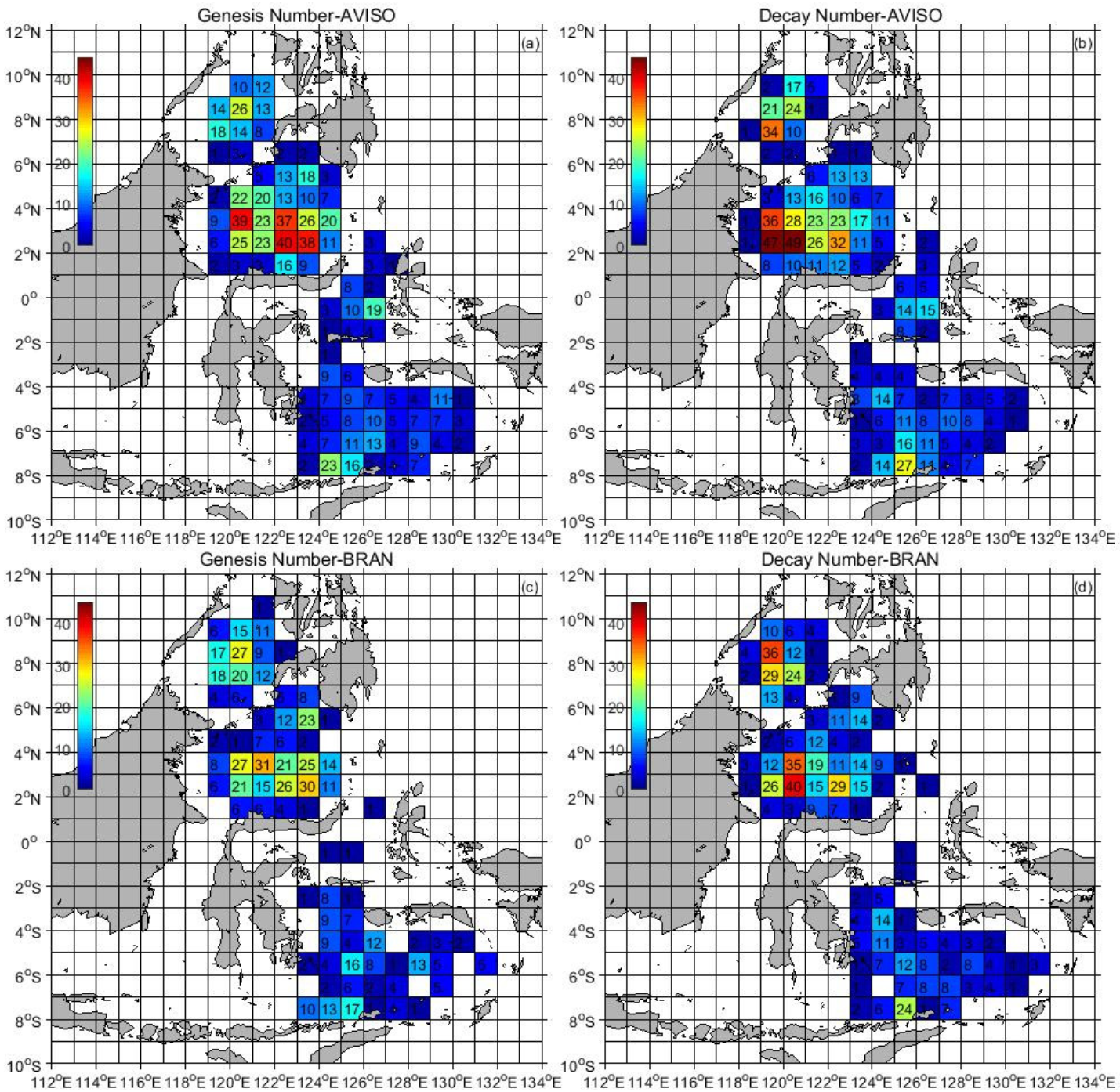
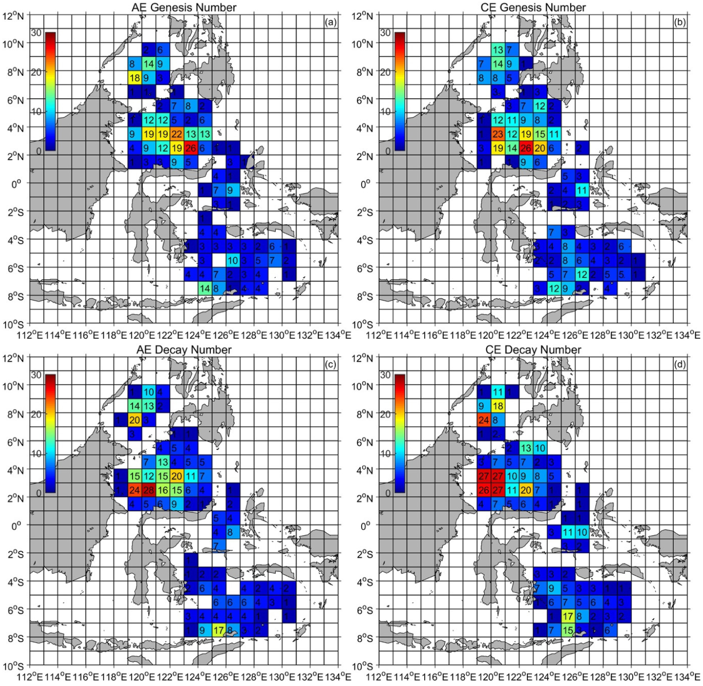
3.1. Eddy Geneis and Decay
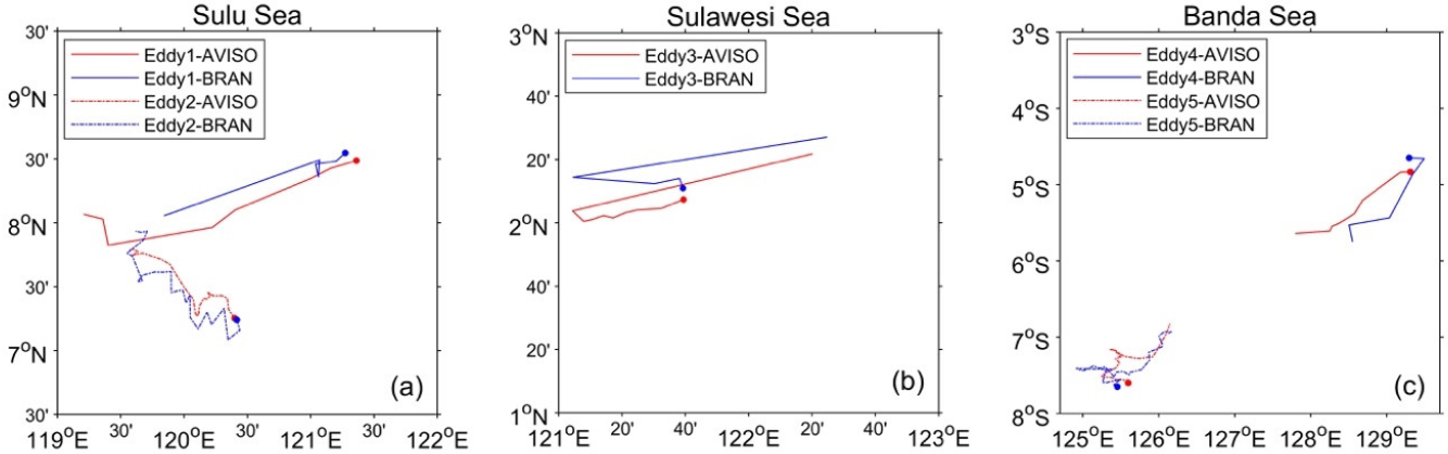
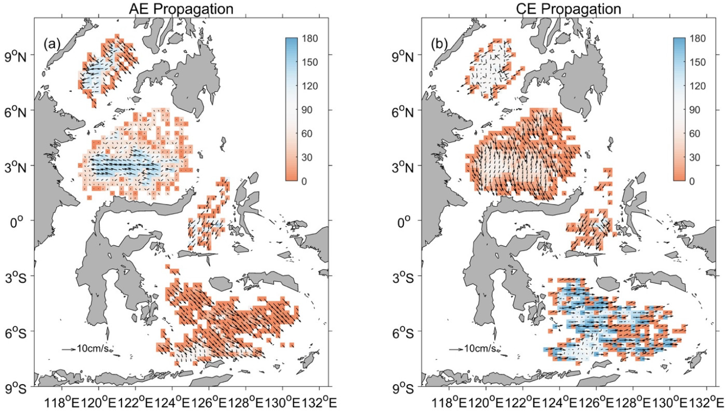
3.2. Eddy Propagation
3.3. Eddy Lifespan
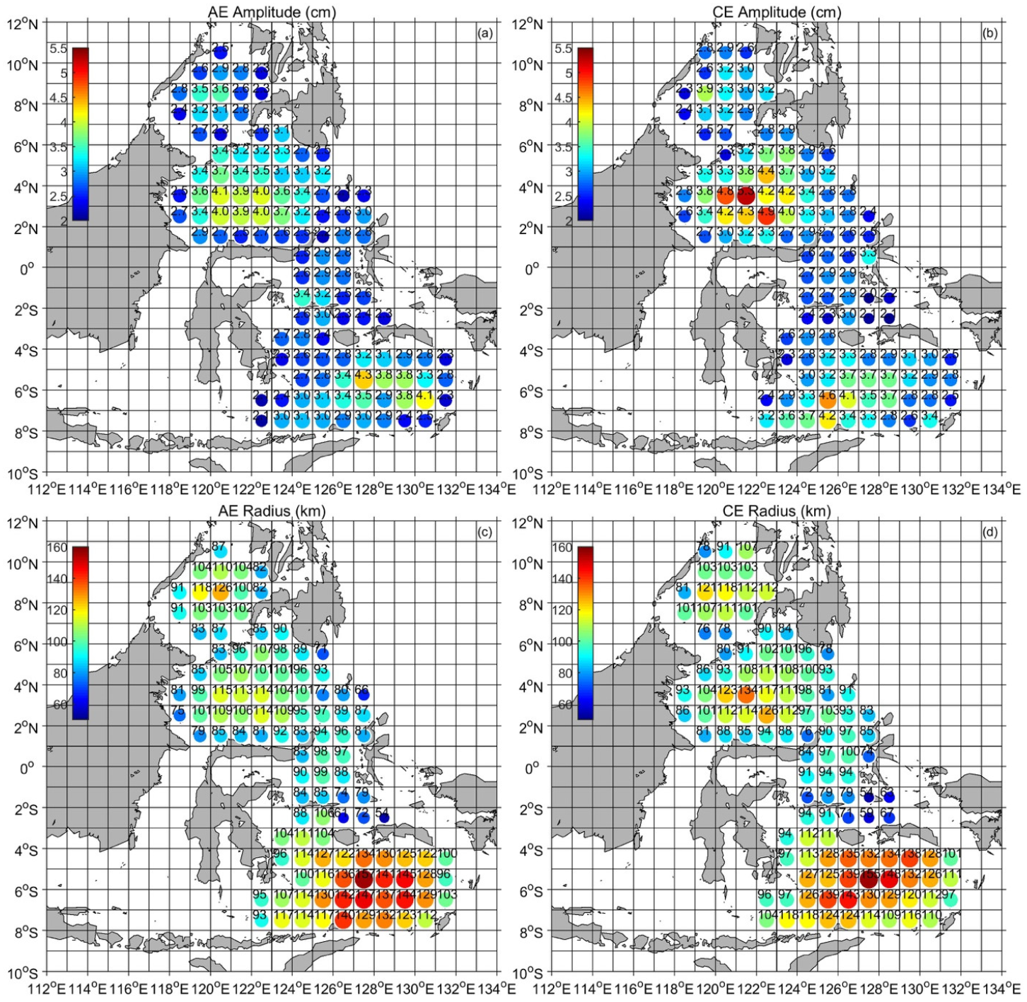
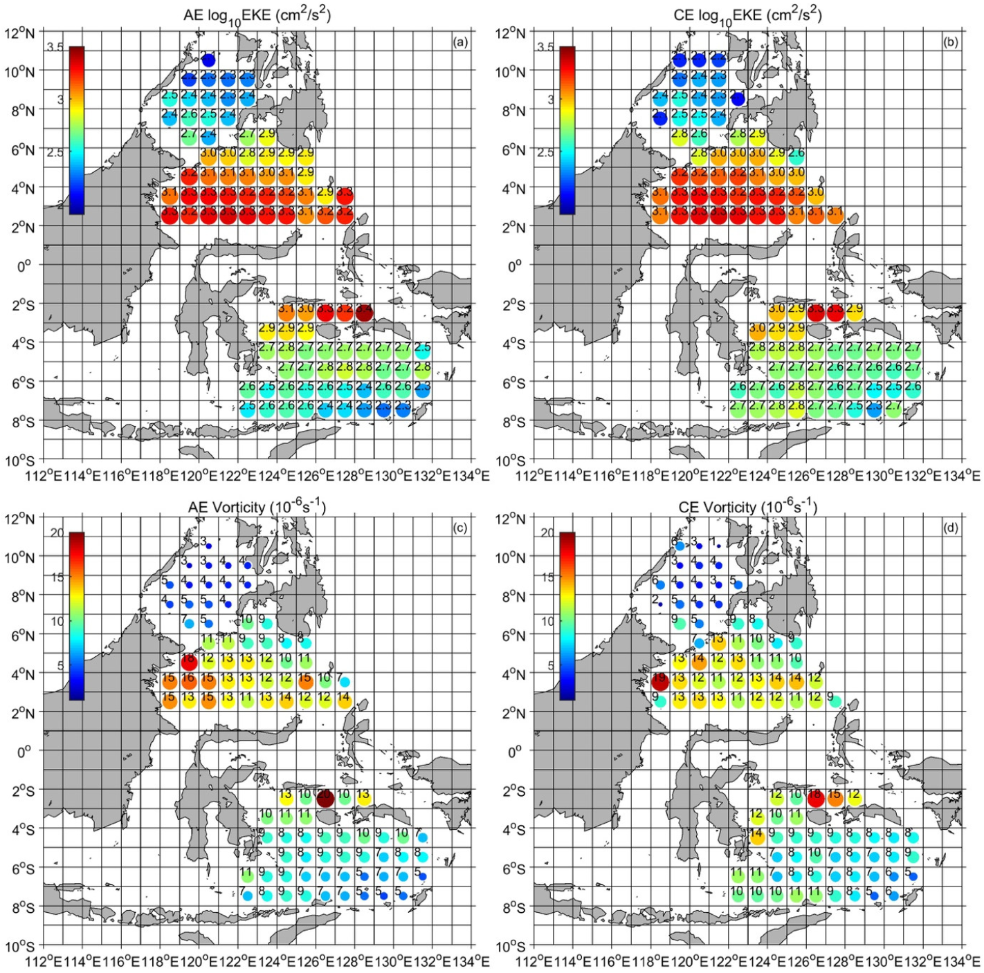
3.4. Distribution of Eddy Properties
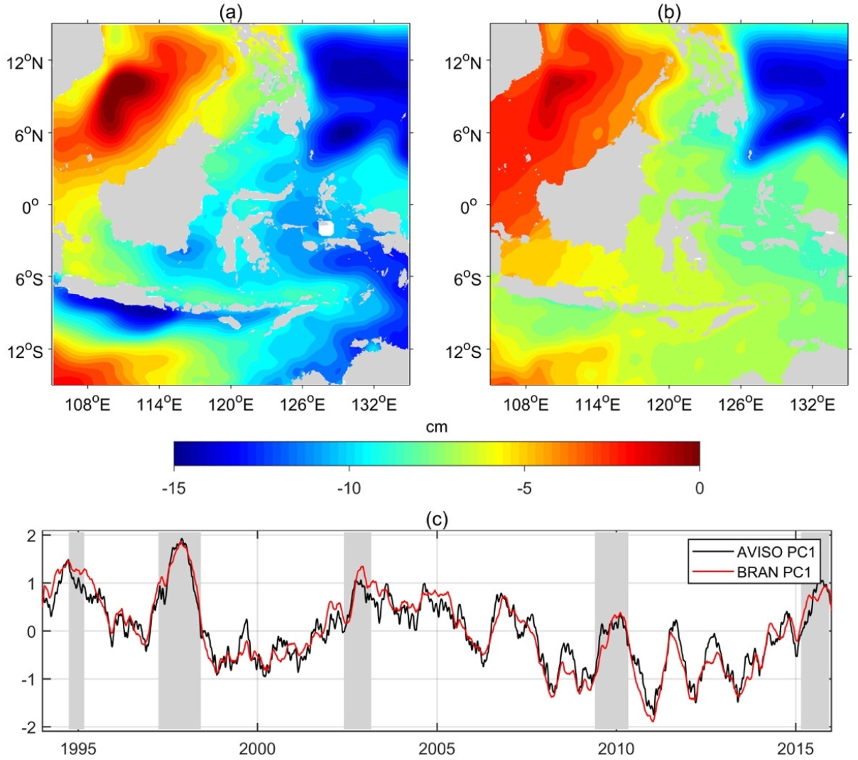
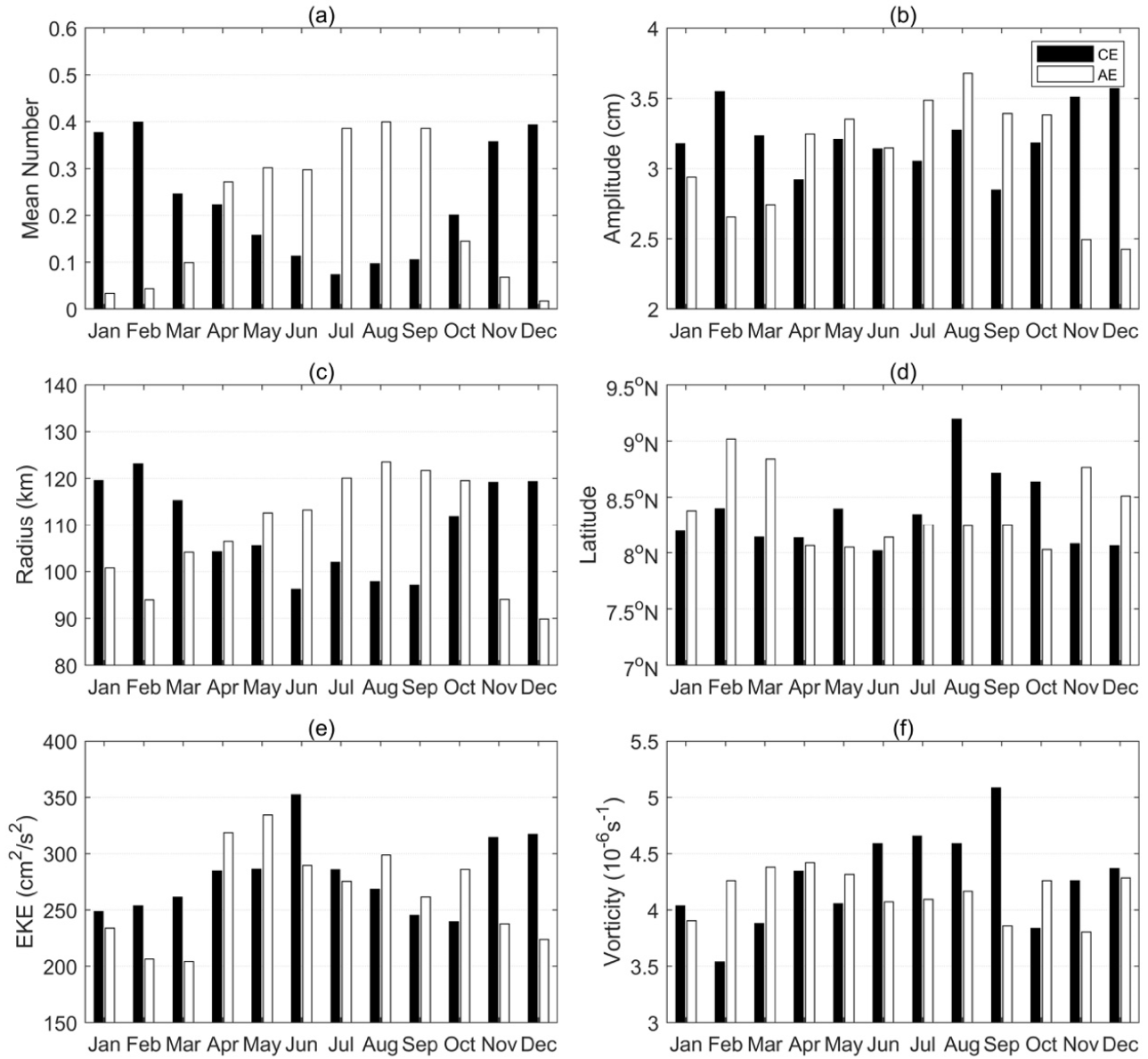
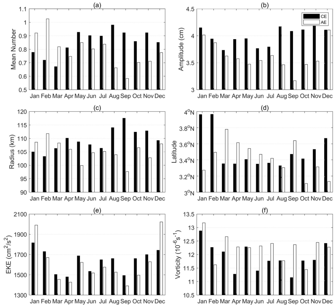
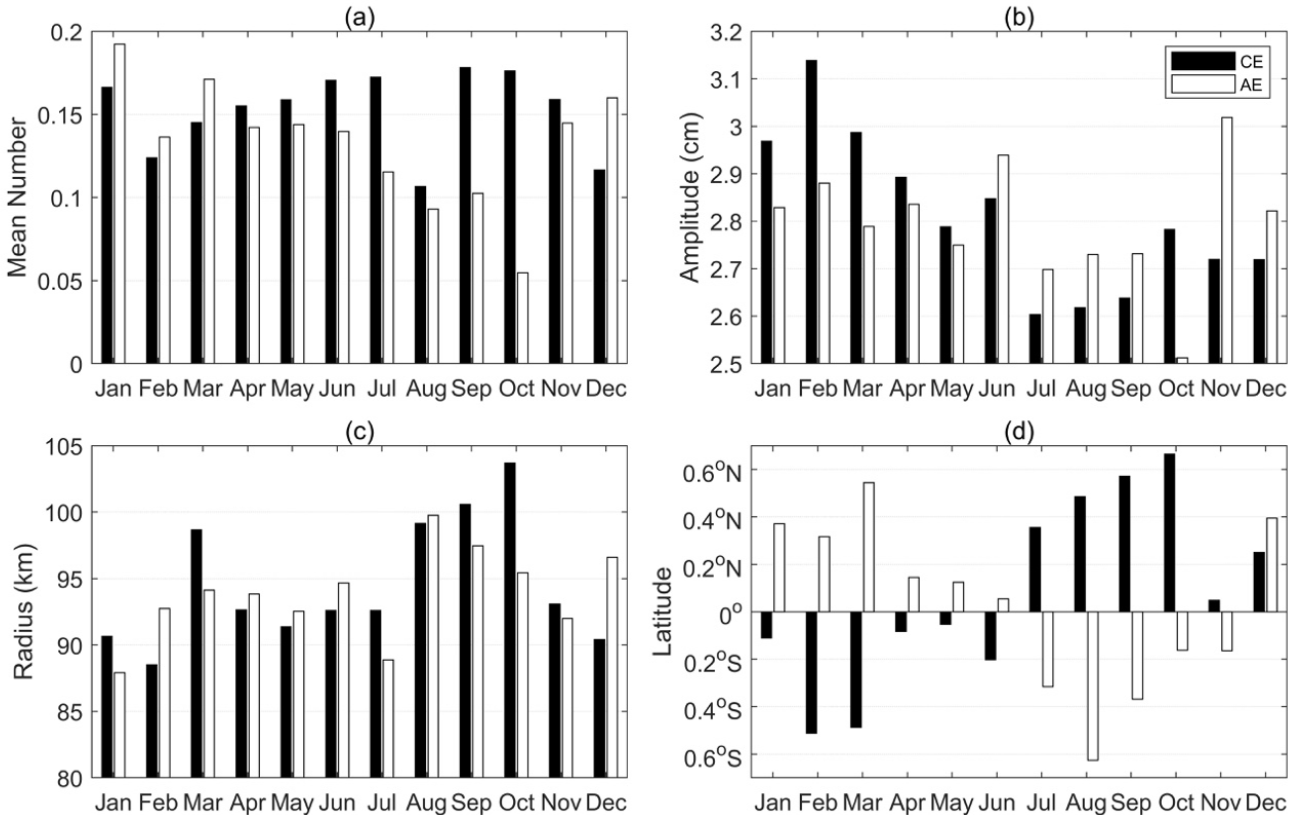
3.5. Seasonal Variability
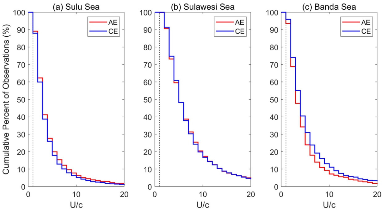
3.6. Eddy Nonlinearity
4. Discussion
5. Conclusions
Supplementary Materials
Author Contributions
Funding
Institutional Review Board Statement
Informed Consent Statement
Data Availability Statement
Acknowledgments
Conflicts of Interest
Appendix A
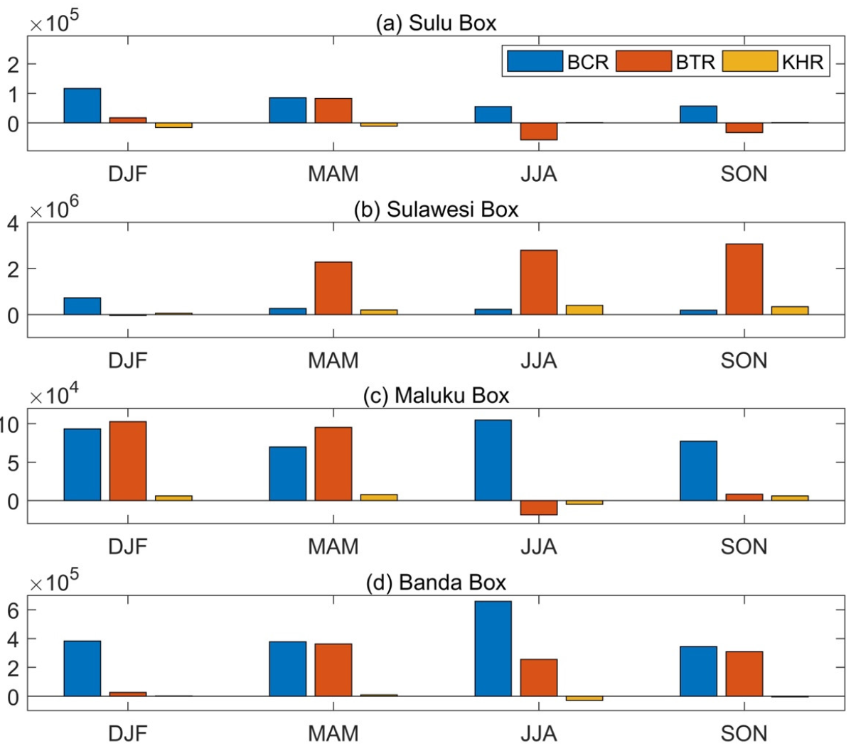
- Sulu Box: , ;
- Sulawesi Box: , ;
- Maluku Box: , ;
- Banda Box: , .

Appendix B
References
- Fu, L.L.; Chelton, D.B.; Le Traon, P.Y.; Morrow, R. Eddy dynamics from satellite altimetry. Oceanography 2010, 23, 15–25. [Google Scholar] [CrossRef] [Green Version]
- Chelton, D.B.; Schlax, M.G.; Samelson, R.M. Global observations of nonlinear mesoscale eddies. Prog. Oceanogr. 2011, 91, 167–216. [Google Scholar] [CrossRef]
- Von Storch, J.S.; Eden, C.; Fast, I.; Haak, H.; Hernández-Deckers, D.; Maier-Reimer, E.; Marotzke, J.; Stammer, D. An estimate of the Lorenz energy cycle for the World Ocean based on the 1/10°STORM/NCEP simulation. J. Phys. Oceanogr. 2012, 42, 2185–2205. [Google Scholar] [CrossRef]
- Kang, D.; Curchitser, E.N. Energetics of eddy-mean flow interactions in the gulf stream region. J. Phys. Oceanogr. 2015, 45, 1103–1120. [Google Scholar] [CrossRef]
- Yan, X.; Kang, D.; Curchitser, E.N.; Pang, C. Energetics of eddy-mean flow interactions along the western boundary currents in the North Pacific. J. Phys. Oceanogr. 2019, 49, 789–810. [Google Scholar] [CrossRef]
- Feng, M.; Wijffels, S.; Godfrey, S.; Meyers, G. Do eddies play a role in the momentum balance of the Leeuwin Current? J. Phys. Oceanogr. 2005, 35, 964–975. [Google Scholar] [CrossRef] [Green Version]
- Zheng, Z.W.; Ho, C.R.; Kuo, N.J. Mechanism of weakening of west Luzon eddy during La Niña years. Geophys. Res. Lett. 2007, 34, 1–5. [Google Scholar] [CrossRef]
- Cheng, Y.H.; Ho, C.R.; Zheng, Q.; Kuo, N.J. Statistical characteristics of mesoscale eddies in the north pacific derived from satellite altimetry. Remote Sens. 2014, 6, 5164–5183. [Google Scholar] [CrossRef] [Green Version]
- Pegliasco, C.; Chaigneau, A.; Morrow, R. Main eddy vertical structures observed in the four major Eastern Boundary Upwelling Systems. J. Geophys. Res. Oceans 2015, 120, 6008–6033. [Google Scholar] [CrossRef]
- Dong, D.; Brandt, P.; Chang, P.; Schütte, F.; Yang, X.; Yan, J.; Zeng, J. Mesoscale Eddies in the Northwestern Pacific Ocean: Three-Dimensional Eddy Structures and Heat/Salt Transports. J. Geophys. Res. Oceans 2017, 122, 9795–9813. [Google Scholar] [CrossRef]
- Cheng, Y.H.; Ho, C.R.; Zheng, Q.; Qiu, B.; Hu, J.; Kuo, N.J. Statistical features of eddies approaching the Kuroshio east of Taiwan Island and Luzon Island. J. Oceanogr. 2017, 73, 427–438. [Google Scholar] [CrossRef]
- Zhang, N.; Liu, G.; Liu, Q.; Zheng, S.; Perrie, W. Spatiotemporal Variations of Mesoscale Eddies in the Southeast Indian Ocean. J. Geophys. Res. Oceans 2020, 125, 1–18. [Google Scholar] [CrossRef]
- Shen, D.; Li, X.; Wang, J.; Bao, S.; Pietrafesa, L.J. Dynamical ocean responses to Typhoon Malakas (2016) in the vicinity of Taiwan. J. Geophys. Res. Oceans 2020. [Google Scholar] [CrossRef]
- Stammer, D. On eddy characteristics, eddy transports, and mean flow properties. J. Phys. Oceanogr. 1998, 28, 727–739. [Google Scholar] [CrossRef]
- Chen, G.; Han, G. Contrasting Short-Lived With Long-Lived Mesoscale Eddies in the Global Ocean. J. Geophys. Res. Oceans 2019, 124, 3149–3167. [Google Scholar] [CrossRef]
- Laxenaire, R.; Speich, S.; Blanke, B.; Chaigneau, A.; Pegliasco, C.; Stegner, A. Anticyclonic Eddies Connecting the Western Boundaries of Indian and Atlantic Oceans. J. Geophys. Res. Oceans 2018, 123, 7651–7677. [Google Scholar] [CrossRef]
- Faghmous, J.H.; Frenger, I.; Yao, Y.; Warmka, R.; Lindell, A.; Kumar, V. A daily global mesoscale ocean eddy dataset from satellite altimetry. Sci. Data 2015, 2, 1–16. [Google Scholar] [CrossRef] [Green Version]
- Chaigneau, A.; Gizolme, A.; Grados, C. Mesoscale eddies off Peru in altimeter records: Identification algorithms and eddy spatio-temporal patterns. Prog. Oceanogr. 2008, 79, 106–119. [Google Scholar] [CrossRef]
- Aguedjou, H.M.A.; Dadou, I.; Chaigneau, A.; Morel, Y.; Alory, G. Eddies in the Tropical Atlantic Ocean and Their Seasonal Variability. Geophys. Res. Lett. 2019, 46, 12156–12164. [Google Scholar] [CrossRef]
- Feng, M.; Zhang, N.; Liu, Q.; Wijffels, S. The Indonesian throughflow, its variability and centennial change. Geosci. Lett. 2018, 5. [Google Scholar] [CrossRef]
- Sprintall, J.; Gordon, A.L.; Wijffels, S.E.; Feng, M.; Hu, S.; Koch-Larrouy, A.; Phillips, H.; Nugroho, D.; Napitu, A.; Pujiana, K.; et al. Detecting change in the Indonesian seas. Front. Mar. Sci. 2019, 6. [Google Scholar] [CrossRef]
- Lukas, R.; Firing, E.; Hacker, P.; Richardson, P.L.; Collins, C.A.; Fine, R.; Gammon, R. Observations of the Mindanao Current during the western equatorial Pacific Ocean circulation study. J. Geophys. Res. 1991, 96, 7089–7104. [Google Scholar] [CrossRef]
- Yuan, D.; Li, X.; Wang, Z.; Li, Y.; Wang, J.; Yang, Y.; Hu, X.; Tan, S.; Zhou, H.; Wardana, A.K.; et al. Observed transport variations in the Maluku Channel of the Indonesian seas associated with western boundary current changes. J. Phys. Oceanogr. 2018, 48, 1803–1813. [Google Scholar] [CrossRef]
- Gordon, A.L.; Napitu, A.; Huber, B.A.; Gruenburg, L.K.; Pujiana, K.; Agustiadi, T.; Kuswardani, A.; Mbay, N.; Setiawan, A. Makassar Strait Throughflow Seasonal and Interannual Variability: An Overview. J. Geophys. Res. Oceans 2019, 124, 3724–3736. [Google Scholar] [CrossRef] [Green Version]
- Van Aken, H.M.; Brodjonegoro, I.S.; Jaya, I. The deep-water motion through the Lifamatola Passage and its contribution to the Indonesian throughflow. Deep. Res. Part I Oceanogr. Res. Pap. 2009, 56, 1203–1216. [Google Scholar] [CrossRef]
- Fang, G.; Susanto, R.D.; Wirasantosa, S.; Qiao, F.; Supangat, A.; Fan, B.; Wei, Z.; Sulistiyo, B.; Li, S. Volume, heat, and freshwater transports from the South China Sea to Indonesian seas in the boreal winter of 2007-2008. J. Geophys. Res. Oceans 2010, 115, 1–11. [Google Scholar] [CrossRef] [Green Version]
- Gordon, A.L.; Huber, B.A.; Metzger, E.J.; Susanto, R.D.; Hurlburt, H.E.; Adi, T.R. South China Sea throughflow impact on the Indonesian throughflow. Geophys. Res. Lett. 2012, 39, 1–7. [Google Scholar] [CrossRef] [Green Version]
- Qiu, B.; Mao, M.; Kashino, Y. Intraseasonal variability in the Indo-Pacific throughflow and the regions surrounding the Indonesian Seas. J. Phys. Oceanogr. 1999, 29, 1599–1618. [Google Scholar] [CrossRef] [Green Version]
- Masumoto, Y.; Kagimoto, T.; Yoshida, M.; Fukuda, M.; Hirose, N.; Yamagata, T. Intraseasonal eddies in the Sulawesi Sea simulated in an ocean general circulation model. Geophys. Res. Lett. 2001, 28, 1631–1634. [Google Scholar] [CrossRef]
- Kashino, Y.; Watanabe, H.; Herunadi, B.; Aoyama, M.; Hartoyo, D. Current variability at the Pacific entrance of the Indonesian Throughflow. J. Geophys. Res. Oceans 1999, 104, 11021–11035. [Google Scholar] [CrossRef]
- Chen, X.; Qiu, B.; Chen, S.; Cheng, X.; Qi, Y. Interannual Modulations of the 50-Day Oscillations in the Celebes Sea: Dynamics and Impact. J. Geophys. Res. Oceans 2018, 123, 4666–4679. [Google Scholar] [CrossRef] [Green Version]
- Kartadikaria, A.R.; Miyazawa, Y.; Nadaoka, K.; Watanabe, A. Existence of eddies at crossroad of the Indonesian seas. Ocean Dyn. 2012, 62, 31–44. [Google Scholar] [CrossRef]
- Yang, C.; Chen, X.; Cheng, X.; Qiu, B. Annual versus semi-annual eddy kinetic energy variability in the Celebes Sea. J. Oceanogr. 2020, 76, 401–418. [Google Scholar] [CrossRef]
- He, Y.; Feng, M.; Xie, J.; Liu, J.; Chen, Z.; Xu, J.; Fang, W.; Cai, S. Spatiotemporal Variations of Mesoscale Eddies in the Sulu Sea. J. Geophys. Res. Oceans 2017, 122, 7867–7879. [Google Scholar] [CrossRef]
- Liu, Y.; Chen, G.; Sun, M.; Liu, S.; Tian, F. A parallel SLA-based algorithm for global mesoscale eddy identification. J. Atmos. Oceans Technol. 2016, 33, 2743–2754. [Google Scholar] [CrossRef]
- Gulakaram, V.S.; Vissa, N.K.; Bhaskaran, P.K. Characteristics and vertical structure of oceanic mesoscale eddies in the Bay of Bengal. Dyn. Atmos. Oceans 2020, 89, 101131. [Google Scholar] [CrossRef]
- Lagerloef, G.S.E.; Mitchum, G.T.; Lukas, R.B.; Niiler, P.P. Tropical Pacific near-surface currents estimated from altimeter, wind, and drifter data. J. Geophys. Res. Oceans 1999, 104, 23313–23326. [Google Scholar] [CrossRef]
- Arbic, B.K.; Scott, R.B.; Chelton, D.B.; Richman, J.G.; Shriver, J.F. Effects of stencil width on surface ocean geostrophic velocity and vorticity estimation from gridded satellite altimeter data. J. Geophys. Res. Oceans 2012, 117, 1–18. [Google Scholar] [CrossRef] [Green Version]
- Yuan, D.; Han, W.; Hu, D. Anti-cyclonic eddies northwest of Luzon in summer-fall observed by satellite altimeters. Geophys. Res. Lett. 2007, 34, 1–6. [Google Scholar] [CrossRef] [Green Version]
- Oke, P.R.; Sakov, P.; Cahill, M.L.; Dunn, J.R.; Fiedler, R.; Griffin, D.A.; Mansbridge, J.V.; Ridgway, K.R.; Schiller, A. Towards a dynamically balanced eddy-resolving ocean reanalysis: BRAN3. Ocean Model. 2013, 67, 52–70. [Google Scholar] [CrossRef] [Green Version]
- Schiller, A.; Oke, P.R.; Brassington, G.; Entel, M.; Fiedler, R.; Griffin, D.A.; Mansbridge, J.V. Eddy-resolving ocean circulation in the Asian-Australian region inferred from an ocean reanalysis effort. Prog. Oceanogr. 2008, 76, 334–365. [Google Scholar] [CrossRef]
- He, Z.; Feng, M.; Wang, D.; Slawinski, D. Contribution of the Karimata Strait transport to the Indonesian Throughflow as seen from a data assimilation model. Cont. Shelf Res. 2015, 92, 16–22. [Google Scholar] [CrossRef]
- Feng, M.; Benthuysen, J.; Zhang, N.; Slawinski, D. Freshening anomalies in the Indonesian throughflow and impacts on the Leeuwin Current during 2010–2011. Geophys. Res. Lett. 2015, 42, 8555–8562. [Google Scholar] [CrossRef] [Green Version]
- Chu, P.C.; Edmons, N.L.; Fan, C. Dynamical mechanisms for the South China Sea seasonal circulation and thermohaline variabilities. J. Phys. Oceanogr. 1999, 29, 2971–2989. [Google Scholar] [CrossRef]
- Cai, S.; He, Y.; Wang, S.; Long, X. Seasonal upper circulation in the Sulu Sea from satellite altimetry data and a numerical model. J. Geophys. Res. Oceans 2009, 114, 1–14. [Google Scholar] [CrossRef]
- Chelton, D.B.; Schlax, M.G.; Samelson, R.M.; de Szoeke, R.A. Global observations of large oceanic eddies. Geophys. Res. Lett. 2007, 34, 1–5. [Google Scholar] [CrossRef]
- Zhan, P.; Subramanian, A.C.; Yao, F.; Hoteit, I. Eddies in the Red Sea: A statistical and dynamical study. J. Geophys. Res. Oceans 2014, 119, 3909–3925. [Google Scholar] [CrossRef] [Green Version]
- Nencioli, F.; Dong, C.; Dickey, T.; Washburn, L.; Mcwilliams, J.C. A vector geometry-based eddy detection algorithm and its application to a high-resolution numerical model product and high-frequency radar surface velocities in the Southern California Bight. J. Atmos. Oceans Technol. 2010, 27, 564–579. [Google Scholar] [CrossRef]
- Penven, P.; Echevin, V.; Pasapera, J.; Colas, F.; Tam, J. Average circulation, seasonal cycle, and mesoscale dynamics of the Peru Current System: A modeling approach. J. Geophys. Res. C Oceans 2005, 110, 1–21. [Google Scholar] [CrossRef]
- Oey, L.Y. Loop current and deep eddies. J. Phys. Oceanogr. 2008, 38, 1426–1449. [Google Scholar] [CrossRef]
- Dufau, C.; Orsztynowicz, M.; Dibarboure, G.; Morrow, R.; Le Traon, P.-Y. Mesoscale resolution capability of altimetry: Present and future. J. Geophys. Res. Oceans 2016, 121, 4910–4927. [Google Scholar] [CrossRef] [Green Version]
- Pujol, M.I.; Faugère, Y.; Taburet, G.; Dupuy, S.; Pelloquin, C.; Ablain, M.; Picot, N. DUACS DT2014: The new multi-mission altimeter data set reprocessed over 20 years. Ocean Sci. 2016, 12, 1067–1090. [Google Scholar] [CrossRef] [Green Version]
- Cai, S.; Su, J.; Gan, Z.; Liu, Q. The numerical study of the South China Sea upper circulation characteristics and its dynamic mechanism, in winter. Cont. Shelf Res. 2002, 22, 2247–2264. [Google Scholar] [CrossRef]
- Bracco, A.; Pedlosky, J. Vortex generation by topography in locally unstable baroclinic flows. J. Phys. Oceanogr. 2003, 33, 207–219. [Google Scholar] [CrossRef] [Green Version]
- Cushman-Roisin, B.; Beckers, J.-M. Introduction to Geophysical Fluid Dynamics: Physical and Numerical Aspects, 2nd ed.; Academic Press: Cambridge, MA, USA, 2011; ISBN 978-0-12-088759-0. [Google Scholar]
- Castruccio, F.S.; Curchitser, E.N.; Kleypas, J.A. A model for quantifying oceanic transport and mesoscale variability in the Coral Triangle of the Indonesian/Philippines Archipelago. J. Geophys. Res. Oceans 2013, 118, 6123–6144. [Google Scholar] [CrossRef]
- Liu, Q.; Feng, M.; Wang, D. ENSO-induced interannual variability in the southeastern South China Sea. J. Oceanogr. 2011, 67, 127–133. [Google Scholar] [CrossRef]
- Zhu, Y.; Wang, L.; Wang, Y.; Xu, T.; Li, S.; Cao, G.; Wei, Z.; Qu, T. Stratified Circulation in the Banda Sea and Its Causal Mechanism. J. Geophys. Res. Oceans 2019, 124, 7030–7045. [Google Scholar] [CrossRef]
- Xu, A.; Yu, F.; Nan, F. Study of subsurface eddy properties in northwestern Pacific Ocean based on an eddy-resolving OGCM. Ocean Dyn. 2019, 69, 463–474. [Google Scholar] [CrossRef] [Green Version]


Publisher’s Note: MDPI stays neutral with regard to jurisdictional claims in published maps and institutional affiliations. |
© 2021 by the authors. Licensee MDPI, Basel, Switzerland. This article is an open access article distributed under the terms and conditions of the Creative Commons Attribution (CC BY) license (http://creativecommons.org/licenses/by/4.0/).
Share and Cite
Hao, Z.; Xu, Z.; Feng, M.; Li, Q.; Yin, B. Spatiotemporal Variability of Mesoscale Eddies in the Indonesian Seas. Remote Sens. 2021, 13, 1017. https://doi.org/10.3390/rs13051017
Hao Z, Xu Z, Feng M, Li Q, Yin B. Spatiotemporal Variability of Mesoscale Eddies in the Indonesian Seas. Remote Sensing. 2021; 13(5):1017. https://doi.org/10.3390/rs13051017
Chicago/Turabian StyleHao, Zhanjiu, Zhenhua Xu, Ming Feng, Qun Li, and Baoshu Yin. 2021. "Spatiotemporal Variability of Mesoscale Eddies in the Indonesian Seas" Remote Sensing 13, no. 5: 1017. https://doi.org/10.3390/rs13051017
APA StyleHao, Z., Xu, Z., Feng, M., Li, Q., & Yin, B. (2021). Spatiotemporal Variability of Mesoscale Eddies in the Indonesian Seas. Remote Sensing, 13(5), 1017. https://doi.org/10.3390/rs13051017