Article

Bottom Detection from Backscatter Data of Conventional Side Scan Sonars through 1D-UNet

1
School of Resources and Environmental Engineering, Anhui University, Hefei 230601, China
2
Anhui Province Engineering Laboratory for Mine Ecological Remediation, Hefei 230601, China
3
College of Civil Engineering, Anhui Jianzhu University, Hefei 230601, China
4
School of Geodesy and Geomatics, Wuhan University, Wuhan 430079, China
5
Institute of Marine Science and Technology, Wuhan University, Wuhan 430079, China
*
Author to whom correspondence should be addressed.
Remote Sens. 2021, 13(5), 1024; https://doi.org/10.3390/rs13051024
Submission received: 13 February 2021 / Revised: 1 March 2021 / Accepted: 5 March 2021 / Published: 8 March 2021
(This article belongs to the Special Issue Deep Learning for Radar and Sonar Image Processing)

Abstract

:
As widely applicated in many underwater research fields, conventional side-scan sonars require the sonar height to be at the seabed for geocoding seabed images. However, many interference factors, including compensation with unknown gains, suspended matters, etc., would bring difficulties in bottom detection. Existing methods need manual parameter setups or to use postprocessing methods, which limits automatic and real-time processing in complex situations. To solve this problem, a one-dimensional U-Net (1D-UNet) model for sea bottom detection of side-scan data and the bottom detection and tracking method based on 1D-UNet are proposed in this work. First, the basic theory of sonar bottom detection and the interference factors is introduced, which indicates that deep learning of the bottom is a feasible solution. Then, a 1D-UNet model for detecting the sea bottom position from the side-scan backscatter strength sequences is proposed, and the structure and implementation of this model are illustrated in detail. Finally, the bottom detection and tracking algorithms of a single ping and continuous pings are presented on the basis of the proposed model. The measured side-scan sonar data in Meizhou Bay and Bayuquan District were selected in the experiments to verify the model and methods. The 1D-UNet model was first trained and applied with the side-scan data in Meizhou Bay. The training and validation accuracies were 99.92% and 99.77%, respectively, and the sea bottom detection accuracy of the training survey line was 99.88%. The 1D-UNet model showed good robustness to the interference factors of bottom detection and fully real-time performance in comparison with other methods. Moreover, the trained 1D-UNet model is used to process the data in the Bayuquan District for proving model generality. The proposed 1D-UNet model for bottom detection has been proven effective for side-scan sonar data and also has great potentials in wider applications on other types of sonars.

Graphical Abstract

1. Introduction

Conventional side-scan sonars have been widely used in many underwater research fields, such as underwater resource exploration, benthic habitat mapping, environmental investigation, seabed target detection, underwater rescue, and archaeology, because of certain advantages like low price and easy installation [1,2,3,4,5]. The conventional side-scan sonar is towed under the water and continuously records the backscatter strength data after the sound waves are projected from the transducer on the port and starboard side. Then, the sonar image constructed using these backscatter strengths can reflect the important information on the seabed, which enables the wide applications for side-scan sonars. In benthic habitat mapping, side-scan sonars can provide the backscatter information from the seabed to construct benthic habitat maps to help protect coastal ocean ecosystems [6,7,8,9,10]. In marine engineering, side-scan sonars are commonly used to detect and track engineering targets, such as offshore pipelines [11]. In the military, side-scan sonars are often used to detect important military targets, such as mines [12,13]. In underwater rescue and archaeology, side-scan sonars can help in detecting important underwater targets, such as human beings [14] and wrecks [15,16]. In the investigation of marine resources and the environment, side-scan sonar images can also be used for resource searching and seabed sediment classification to understand the environmental changes of the seabed [17,18,19].
The sonar depth can be measured by the depth sensor when the side-scan sonar is towed underwater. However, the sonar height to the sea bottom needs to be obtained by the bottom detection method. The side-scan sonar can find the sea bottom position by detecting the maximum backscatter strength within a certain range, and the sonar height to the sea bottom can be calculated by the sample interval and the sound speed [20]. The main purpose of conventional side-scan sonars is to obtain seabed images. Hence, the image quality is more important in side-scan sonar operation rather than sounding, and the backscatter strengths are compensated by time-varying gains to offset the propagation loss of side-scan sonars [21,22]. The time-varying gains for side-scan data are often unknown due to sonar self-limitation or improper recording operations, which would bring problems in the bottom detection. In addition, other interference factors, including the sonar self-noise generated when the sonar is close to the vessel in the shallow water area, the possible suspended objects in the water column, and the possible targets on the seabed will also bring problems in the bottom detection of side-scan sonar data.
Detecting the sea bottom from the conventional side-scan sonar data using the traditional method is difficult due to these interference factors. Accordingly, commercial programs mostly provide manual assistance functions using the various threshold parameter settings to improve bottom detection results. The parameter setup needs great human intervention to accommodate different types of side-scan data and makes the real-time operation unfeasible. The other solution is to covert the time-domain side-scan data into frequency-domain sequences [23]. Then, the bottom position can be found using the mathematical characteristics [24] in the frequency-domain sequences. However, some interference factors may have similar mathematical characteristics, so the robustness of these characteristics to noise must be improved. Considering the consistency principle of seafloor terrain variation, other methods apply dynamic post-processing methods [25], such as the Kalman filter to improve the accuracy of the bottom detection and tracking results [26]. However, real-time bottom detection and tracking become difficult when many post-processing operations are used.
Deep learning methods have been widely applied in related research fields [27,28,29,30,31,32] and could be a better choice in realizing real-time and accurate bottom detection of side-scan data affected by numerous interference factors [33]. The backscatter strengths will represent a special variation characteristic when the sound reaches the sea bottom. If the deep learning model can accurately distinguish the variation characteristic from other interference factors, then the bottom detection can be realized [34]. In addition to processing two-dimensional (2D) images, deep learning methods have been also applied in target recognition and segmentation of the one-dimensional (1D) sequences [35,36] and three-dimensional (3D) images [37,38]. The 1D convolutional neural network (1D-CNN), as an effective recognition and classification model for 1D sequence data, has been applied to recognize the backscatter strength sequences at the bottom positions to fulfill the seabed detection and tracking of side-scan sonar data [39]. However, 1D-CNN must traverse the ping sequence to recognize the bottom position and would cost a substantial amount of time in some cases and bring delays in real-time operations. Moreover, recognition of local sequence variation will lose the perception of the whole sequence variation and make the model insufficiently robust to some interference factors. The U-Net-type models are widely used in object segmentation because they can simultaneously perceive the whole and local features [40,41]. The one-dimensional U-Net (1D-UNet) model has been proven to be suitable for sequence segmentation [42]. Therefore, a 1D-UNet model is proposed and applied to segment the bottom positions from side-scan backscatter data to realize the bottom detection and tracking in this work. The major contributions of this work include:
  • The interference factors of bottom detection, including compensation with unknown gains, sonar self-noise and vessel noise, suspended objects in the water column, and targets on the seabed, are introduced in detail.
  • A well-designed 1D-UNet model for the bottom detection of the side-scan backscatter sequences is proposed and validated in the experiment with high accuracies and good robustness to the interference factors.
  • The proposed bottom detection and tracking method of side-scan data has been proved to have fully real-time performance and show potentials in wider applications on other types of sonars.
In this paper, the traditional bottom detection theory is first introduced, and the interference factors that bring problems in bottom detection of side-scan data are listed. Second, the structure and implementation of the proposed 1D-UNet model are introduced in detail. Third, the bottom detection and tracking methods using the 1D-UNet model are presented. In the experimental part, the measured side-scan sonar data in Meizhou Bay and Bayuquan District were used to validate the model and methods.

2. Theory and Method

This chapter contains three parts. The first part introduces the bottom detection theory of conventional side-scan sonars and main interference factors. The second part provides the proposed 1D-UNet model for sea bottom detection of side-scan backscatter strength sequences. The third part is the sea bottom detection and tracking method of successive pings.

2.1. Bottom Detection of Conventional Side-Scan Sonars and Main Interference Factors

Conventional echo sounders measure depth by generating a short pulse of sound and detecting the pulse-echo from the bottom. After the sound is projected from the transducer, the sound first propagates in the water column. The backscattering strength from the water will be low because the water column mainly contains water. Then, the sound will be reflected and refracted when the sound pulse reaches the sea bottom. At this time, an echo with a strong backscatter strength will be received by the transducer. Considering the propagation loss of the sound wave, this high-sound-level echo is often the strongest in the detection gates. This is the basic bottom detection principle of echo sounders.
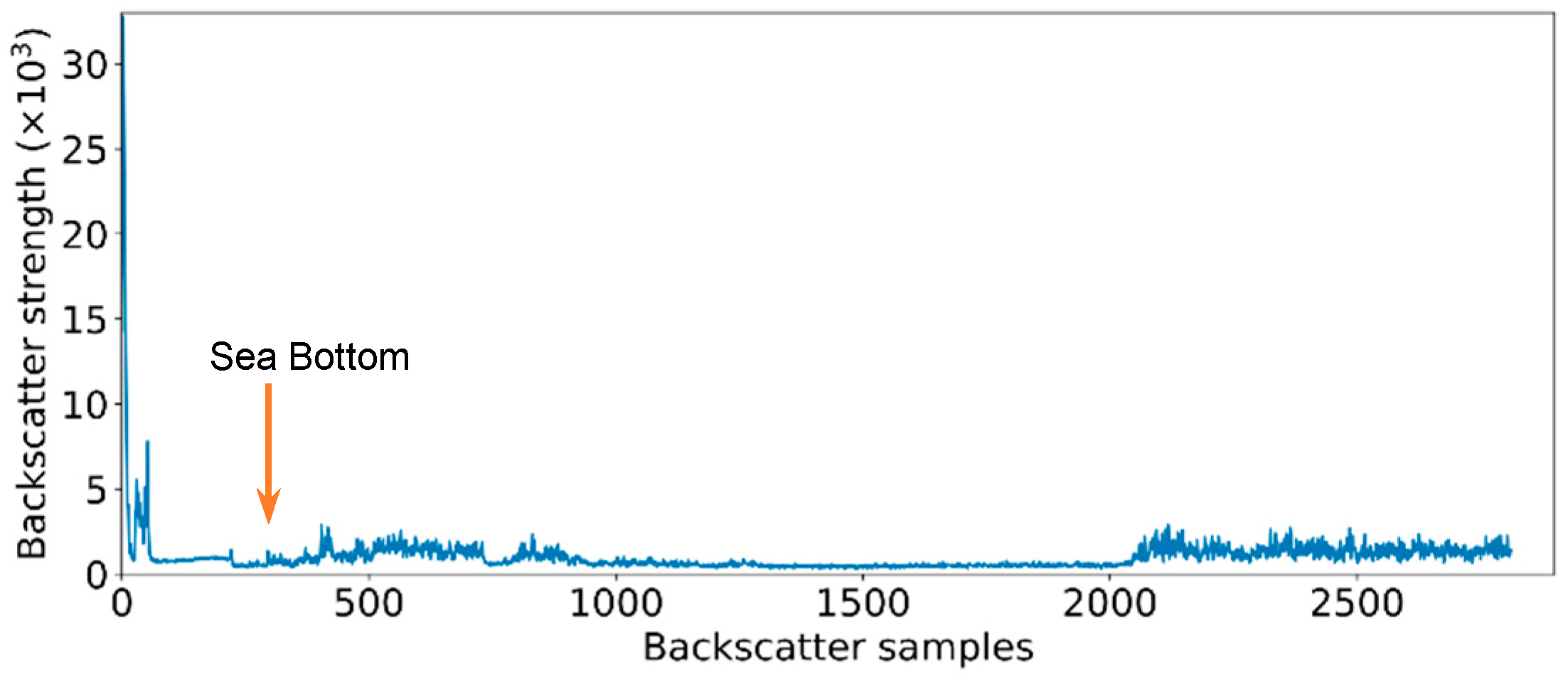
Similar to echo sounders, the side-scan sonar transducer projects a single wide sound beam at the port and starboard sides and records the backscatter strengths in the time sequence on the port and starboard sides. The backscatter strength sequences of the port and starboard sides are independent and relatively symmetric and can be separately processed to detect the sea bottom. Under ideal conditions, the transducer would record the highest-level echo when the sound hits the sea bottom; accordingly, the bottom detection process can be easily conducted. However, the traditional bottom detection principle could fail on the effects of unknown gain, sonar self-noise and beam patterns, suspended objects in the water column, target on the seabed, random noises, and other exceptional situations, which will introduce difficulties in bottom detection of side-scan data (Figure 1).
In Figure 1b, these influencing factors that bring difficulties in bottom detection of side-scan data include:
  • Unknown gain. During the sound propagation, the level of the sound wave gradually decreases due to the effect of propagation loss. When the sound wave reaches the sea bottom, the transducer will record a high-level echo, which shows the sea bottom position. Given that the side-scan sonars are mainly used for obtaining seabed images, time-varying gains are applied on the side-scan backscatter samples to make the strengths uniform. In many cases, the gains are unknown because the instrument does not provide it, or the operator does not record it. The unknown gain will cause the echoes arriving at the sea bottom to be no longer the highest-level echoes, which brings problems to the traditional methods.
  • Sonar self-noise and vessel noise. The self-noises of side-scan sonars include the noises of the sonar itself (such as ringing error) and the survey ship. In some shallow waters, the ship noise will also bring great influence to the side-scan sonar when the side-scan sonar is installed on the ship or towed near the ship. This type of noise is mainly concentrated within a certain range after the sound is emitted.
  • Suspended objects in the water column. Fishes, marine suspended matters, bubbles, and other suspended objects may appear and bring effects on bottom detection during the sound wave propagates on the water column before reaching the seabed. The echoes from these suspended objects have a relatively larger sound level than echoes from water, which shows a similar strength variation when the sound reaches the sea bottom. Thus, the suspended objects in the water column are potential influencing factors.
  • Targets on the seabed. After the sound reaches the seabed, the side-scan sonar will continuously record the backscatter strengths of echoes from the seabed, which are used for constructing the seabed sonar image. When a target appears on the seabed, the echoes from the target could have a much larger sound level than echoes for the surrounding seabed and would be an influencing factor of bottom detection.
  • Random noises and exceptional situations. Random noises are also likely to produce abnormally strong-level echoes, similar to echoes when the sound hits the sea bottom. In exceptional situations, side-scan sonar data may be recorded incomplete or completely missing. These situations can also cause problems in the bottom detection of side-scan sonar data.
The traditional bottom detection method of side-scan data could be ineffective due to these interference factors. Nevertheless, the special variation characteristics in sound levels (or backscatter strengths) when the sound arrives at the seabed are distinguishable with those of these interference factors, which can serve as the basis for bottom detection of side-scan sonar data. Therefore, the proposed model that can detect the special strength variation characteristics is presented below.

2.2. 1D-UNet for Bottom Detection

The regional backscatter strength sequence around the sea bottom position shows a special variation feature, as illustrated in Figure 1. So, the 1D-UNet model is proposed to segment the bottom positions from the side-scan backscatter sequences. In this section, the sampling steps including extraction from the raw data, normalization, and bottom positions labeling are introduced first. Then, the structure and implementation of the 1D-UNet model are explained in detail. The flow chart of the proposed 1D-UNet model is shown in Figure 2.

2.2.1. Samples

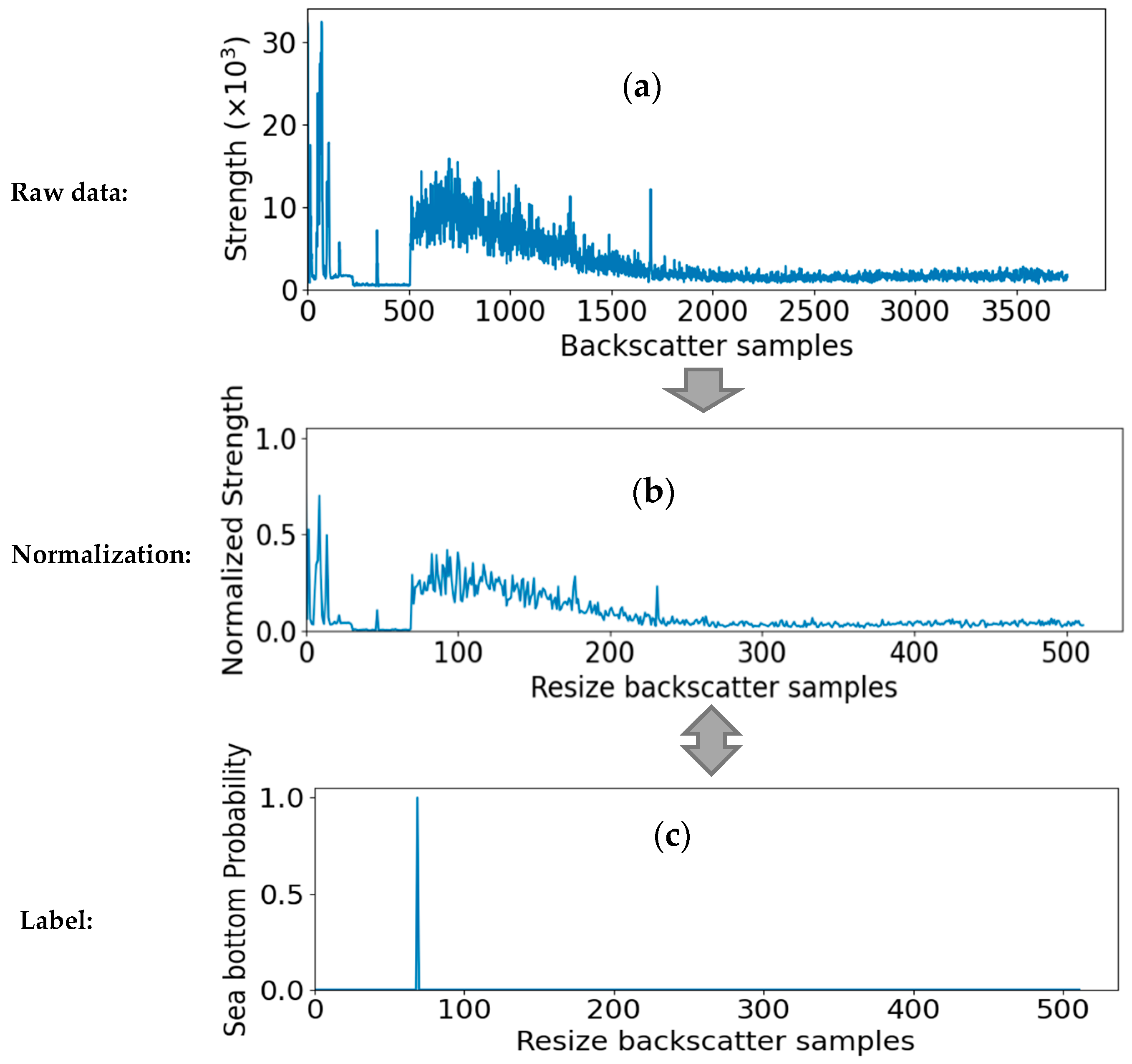
Diverse side-scan sonars record backscatter strengths in different ranges and use various sample rates (Figure 3a). To learn the sea bottom position from these data via deep learning models, samples should be normalized into (0–1) and resized to a fixed size (powers of two, such as 512). The variation features of the backscatter strengths would not be changed after the normalization. The samples of each backscatter strength sequence can be normalized using the maximum and minimum values of each sequence as follows:
d B N = d B d B m a x d B m a x d B m i n
where dBN is the normalized strength of the backscatter sample; dB is the raw strength; and dBmax and dBmin are the maximum and minimum values of the strength sequence, respectively.
To use the 1D-UNet model to segment the sea bottom position of the side-scan backscatter sequence, the model should be able to learn the correct relationship between the one-ping port-side (starboard-side) backscatter strength sequence (Figure 3b) and the corresponding sea bottom position (Figure 3c). The input data of 1D-UNet are the normalized backscatter strength sequences (Figure 3b). Meanwhile, the output sequences are the corresponding sea bottom probabilities of each backscatter sample (Figure 3c).
The corresponding bottom positions of each backscatter strength sequence can be detected using the traditional method and should be manually checked to ensure accuracy. The target sequence of the 1D-UNet has the same size as the input sequence. The value at the sea bottom position should be set as one, while those at the other positions should be zero (Figure 3c).

2.2.2. Structure of 1D-UNet

The 1D-UNet is the 1D version of famous U-Net models and can fulfill the subsequence segmentation of the 1D data sequence, and is used for sea bottom detection of side-scan backscatter strengths in this work. The 1D-UNet model contains the decoding and encoding parts. In the encoding parts, the input sequences were downsampled to extract the features. In the decoding parts, the learning features were upsampled to the output results.
Input data and output target: The input layer is the backscatter strength sequences that were normalized and resized as 1 × 512 1D tensors with a range from zero to one. The backscatter strength sequences were downsampled using 1D convolution and 1D pooling operations from 1 × 512 tensors to 1024 × 32 tensors. Then, the tensors were upsampled using 1D transposed convolution, concatenation, and 1D convolution from 1024 × 32 tensors back to 1 × 512 tensors. The output layer is the corresponding probability sequences of bottom detection with a range from zero to one. The 1D-UNet structure is shown in Figure 4.
Encoding part: The layers of the encoding part are composed of 1D convolution and pooling operations. The 1D convolution operation s of the data sequences in discrete form is shown below.
s ( t ) = ( d w ) ( t ) = a = d ( a ) w ( t a )
where d is the input data sequence, w is the activation function, and t is the tth value of d.
The convolution operation will reduce the size of the tensor on the original dimension. To make the concatenation operation easier and ensure the size consistency between the final output and the input layer, we add padding for each convolution operation based on the convolution kernel size. Therefore, the size after each convolution operation is always a multiple of two. The convolution operation is followed by the activation function. The rectified linear unit (ReLU) h is selected as the activation function for the convolution layers.
h w , b ( X ) = max ( X · w + b , 0 )
where w and b are the trainable parameters, and X is the input data.
A pooling function replaces the layer output at a certain location with a summary statistic of the nearby outputs, in order to reduce the number of parameters to learn and the amount of computation performed. Here, the max-pooling operation is used to obtain the maximum output within a rectangular neighborhood.
Decoding part: The layers of the decoding part are composed of 1D transposed convolution (up-sampling), concatenation, and convolution operations. After processing by the encoding part, the original-dimension length of the input sequence has reduced from 512 to 32. The length needs to increase back to 512 to predict the corresponding bottom position. The transposed convolution (or deconvolution [43]) broadcasts input values through the kernel and results in a larger output shape, which would serve this purpose.
To avoid losing important information during down-sampling operations, 1D-UNet uses skip-connections via the concatenation of the same-size layers in the encoding and decoding parts for perceiving both of the low-level and high-level features of the input sequence. After concatenation, the first-dimension length of the sequence will be doubled. Accordingly, the convolution operations are applied to reduce the size. Therefore, the size of the output sequence is the same as the input data after processing by the decoding part.
Loss function: After each training loop, the loss function is used to calculate the difference between the predicted results and the ground truth data. Given that the bottom detection problem is a sequence segmentation task, the output sequences only contain two classes (1 foreground/bottom, 0 background) and the classes are quite imbalanced. To handle the class-imbalance problem [44], the mean squared error (MSE) function between the predicted result and the target sequence is selected as the loss function.
M S E = 1 N i = 1 N ( y i y ^ i ) 2
where N is the length of the predicted and target sequences, yi is the ith sample of the predicted sequence, and y ^ i is the ith sample of the target sequence.
Since the background scores are 0, the value of the MSE loss function is always affected by the foreground (bottom) scores. Therefore, the 1D-UNet model can be trained successfully with good accuracy.
Optimizer: Base on the loss function, the optimizer is intended to update the model parameters to reduce the loss and improve the accuracy. The root mean square propagation optimizer, as one of the current most important optimizers, which uses the adaptive learning rate and has good robustness in most problems, was chosen as the optimizer for 1D-UNet to update the parameters.
Accuracy: The training and validation accuracies (accT and accV) of the model are calculated as the proportions of the correct-detected sample number in the total training and validation sample number, respectively, as shown in Equation (5) below:
a c c T = N 1 N T ,   a c c V = N 2 N V
where N1 and NT are the numbers of correct-predicted and total training samples, and N2 and NV are the numbers of correct-predicted and total validation samples.
Considering the sample accuracy using the traditional method with manual correction, the correctness of each prediction result can be determined true if the difference between the location of the maximum bottom probability in the output sequence and the labeled position is within 0.5% of the output sequence length, as
correct ( y ) = { t r u e , a b s ( i y i y ^ ) ) 0.5 % × l y f a l s e , a b s ( i y i y ^ ) ) > 0.5 % × l y
where y and y ^ are the predicted and the target sequences, iy and i y ^ are the index of the maximum probabilities in the predicted and target sequences, ly is the length of the predicted sequence, and abs means the absolute value function.
During continuous training and learning from the relationship between the input sequences and the output targets, the training and validation losses of the 1D-UNet will decrease, and the training and validation accuracies will increase. The well-trained 1D-UNet model serves as the basis of sea bottom detection and tracking of side-scan pings.

2.3. Sea Bottom Detection and Tracking of Side-Scan Pings

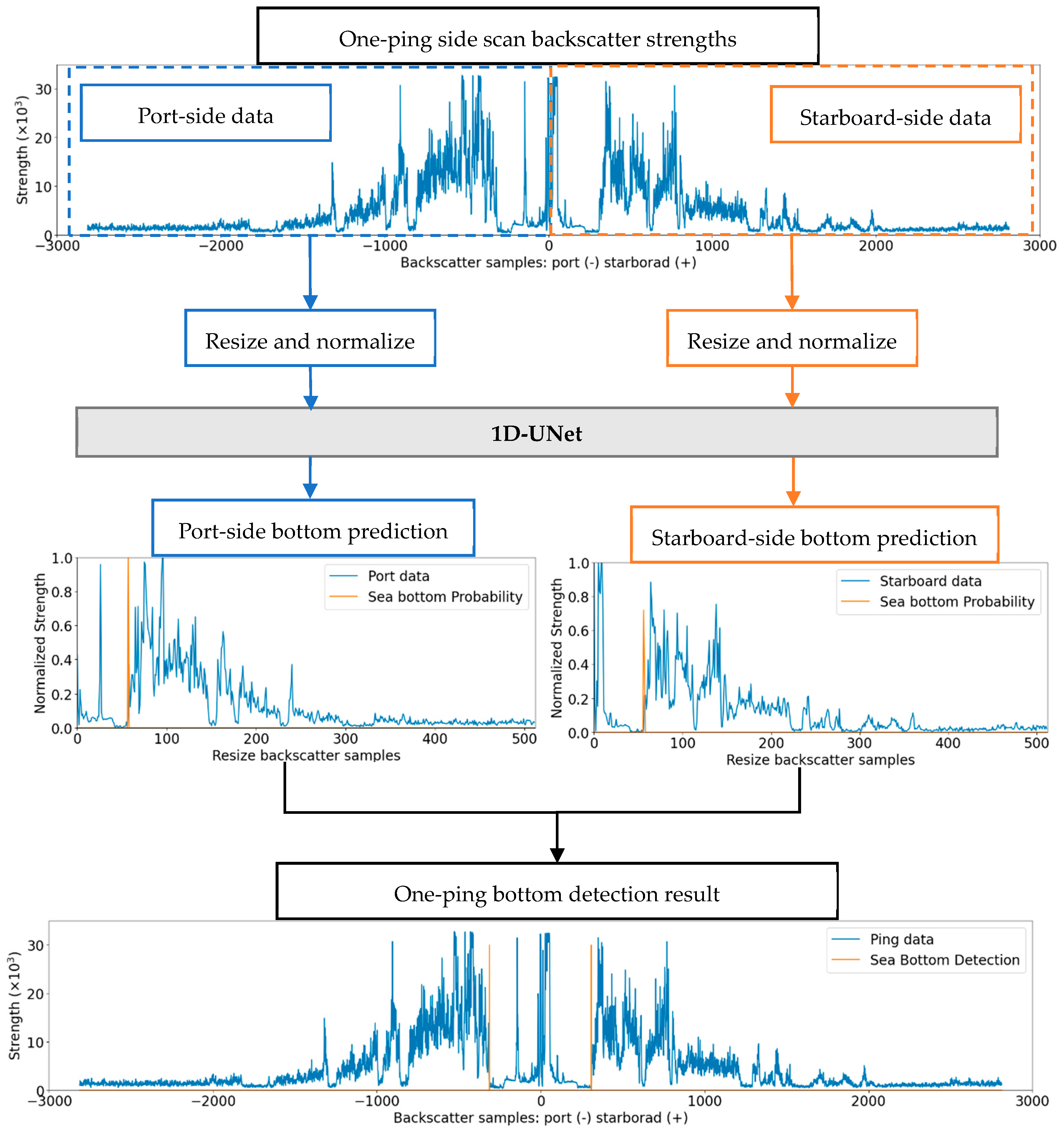
After the 1D-UNet model establishment, the trained 1D-UNet model is used for predicting the bottom position of each side-scan ping data (Figure 5).
Each side-scan ping has the port and starboard part. The port-side and starboard-side data should be separately processed. The port-side (starboard-side) backscatter strength sequences need to be resized and normalized as the input data. Then, the bottom positions on both sides are predicted using 1D-UNet. After determining the sea bottom positions of the port-side and starboard-side backscatter strength sequences, the sea bottom of the ping data can be obtained.
When the seabed is almost flat, the port and starboard sea bottom position should be nearly the same. Given the symmetry between the port and starboard data, the predicted port and starboard bottom positions can be combined to check the exceptional results and achieve better robustness. Some side-scan sonars have two or more frequencies. Thus, the ping data of the low and high frequency should be processed separately.
In the practical fieldwork, the side-scan sonar constantly records the backscatter strength data of each ping. According to the operation principles of side-scan sonars, these successive pings following the along-track direction can be processed by the proposed 1D-UNet model to fulfill real-time bottom detection. The bottom tracking of the side-scan sonar data can be fulfilled via continuous bottom detection of successive pings. The bottom detection and tracking procedure of continuous pings are shown in Figure 6. The bottom detection accuracy of successive pings can be calculated as follows:
a c c = N c N 0
where acc means accuracy, Nc is the number of correct-bottom-detection pings, and N0 is the total number of pings.

3. Experiment and Results

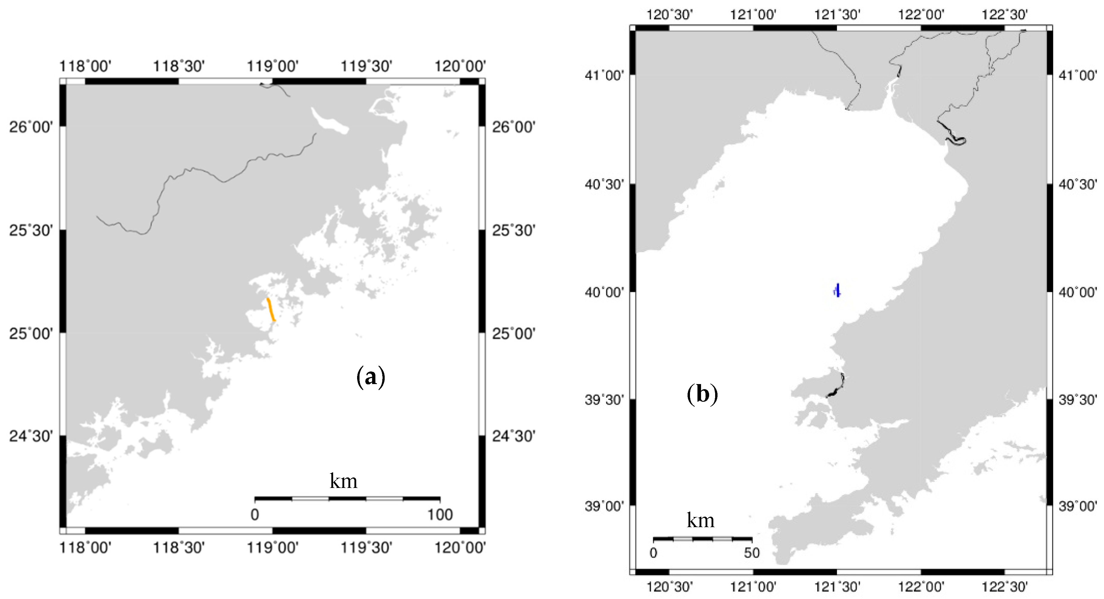
To verify the validity and performance of the proposed 1D-UNet in this work, the measured side-scan sonar data in Meizhou Bay, Fujian, China 2012 and Bayuquan, Liaoning, China, 2014 were selected for the experiment (Figure 7).
In Meizhou Bay, an Edgetech 4100P side-scan sonar was used for the measurement, with an operation frequency of 500 kHz, a maximum sampling slant range of 150 m, and ping interval time of 150 ms. The side-scan data in the Bayuquan District were obtained with an Edgetech 4200 side-scan sonar, with an operating frequency of 400 kHz, maximum sampling slant range of 150 m, and ping interval time of 210 ms. These side-scan data were all recorded in eXtended Triton Format (*.xtf) files, which only contained the compensated backscatter strengths in each ping data, while the raw signal levels and the time-varying gains are unknown. The experiment contains three parts:
  • Training and validation of 1D-UNet. The side-scan data containing 13,504 pings from a survey line in Meizhou Bay were selected for the 1D-UNet training and validation. The sampling and training processes were given in detail. The predicted bottom results were compared with the target bottom results, and the model accuracy was validated via statistical analysis. The 1D-UNet model was further validated by using the side-scan data of other survey lines in the same region.
  • Model comparison. The trained 1D-UNet model was compared with other methods: The 1D-UNet model was compared with the last peak and the 1D-CNN method to process the side-scan data with different interference factors. The real-time performance of the 1D-UNet model was compared with 1D-CNN via statistical analysis.
  • Bottom detection in a different region. To prove the generality of the 1D-UNet model, the trained 1D-UNet model using the side-scan data in Meizhou Bay was applied to process those data in the Bayuquan, where the data were measured with a different side-scan sonar model.
The pre-processing stages including decoding raw binary files and sampling from the side-scan files were processed using our self-developed programs written in C++. The proposed 1D-UNet model was implemented using the Python language (version 3.8) on PyTorch 1.7.1 library with CUDA 11.0 support. The bottom detection and tracking of side-scan pings were also written in Python. The experiments were carried on a desktop computer having a 64-bit Windows 10 operating system with an AMD Ryzen 5 2600X processor, 64 GB RAM, and a Nvidia RTX 2700 GPU. The 1D-UNet model was trained and validated on the Nvidia GPU with CUDA support for acceleration.

3.1. Training and Learning from the Side-Scan Data in Meizhou Bay

3.1.1. Training and Validation of the 1D-UNet Model

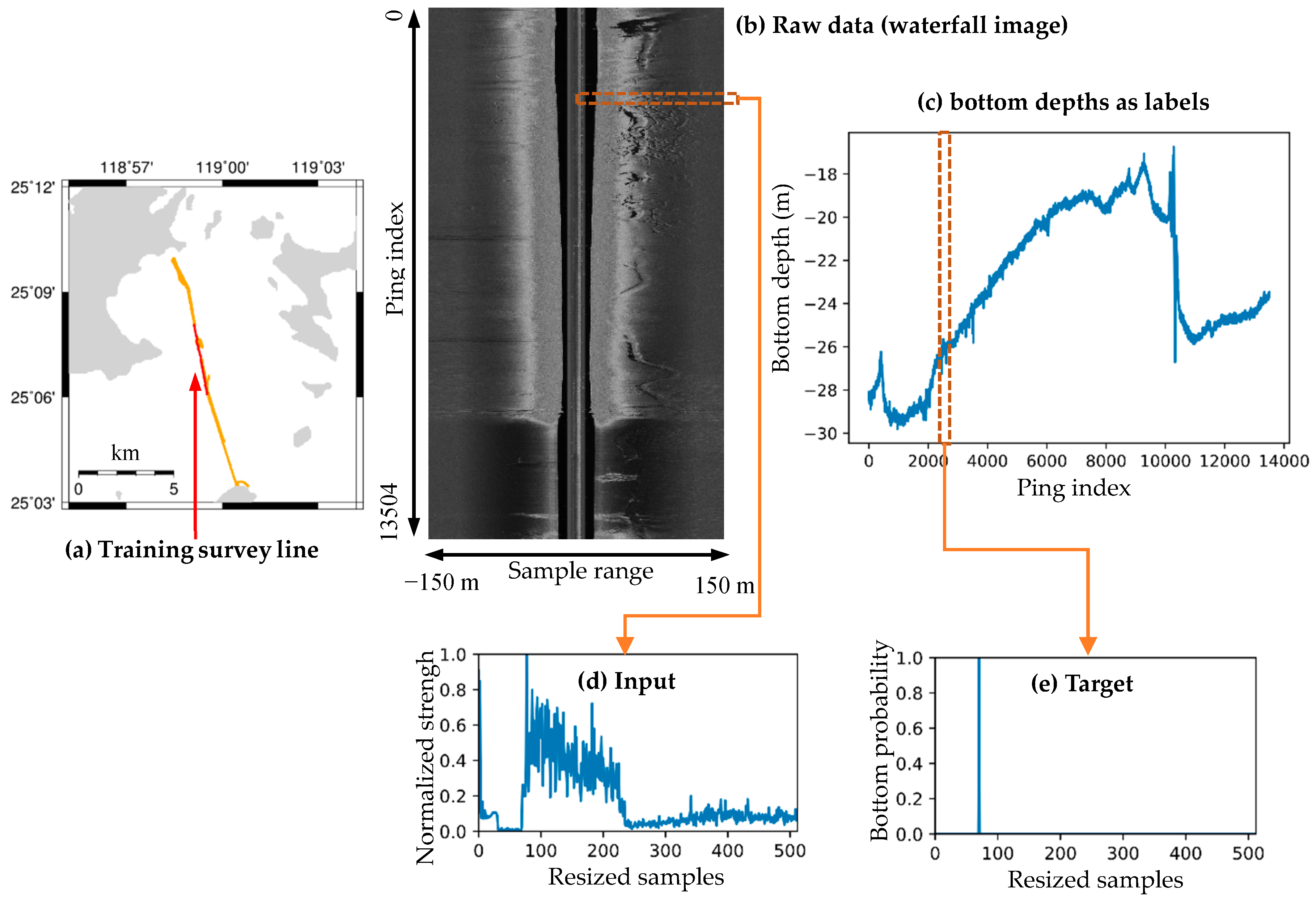
The training of the 1D-UNet model requires a large amount of sample data to obtain high accuracy and generality. First, a survey line with 13,504 pings was selected for the model training (Figure 8a). The raw side-scan data (as *.xtf files) were decoded, and the corresponding waterfall image was constructed (Figure 8b). The corresponding bottom detection results were processed by manual recognition (Figure 8c).
The waterfall image (Figure 8b) shows that the backscatter strengths of this survey line have been compensated with time-varying gains; thus, the maximum-strength echoes were not at the position where the sound waves hit the bottom. The survey line spans the seabed with two different types of sediments. Accordingly, the backscatter strengths greatly varied from different sediments. At the connection region of different sediments, the seabed topography fluctuates, which could bring some challenges to bottom detection and tracking. A band-shaped noise appears at the center of the waterfall image, which indicates the existence and effects of sonar self-noise and vessel noises. Moreover, the obvious targets on the seabed could also be the interference factor to the bottom detection.
The port-side and starboard-side backscatter sequences can be used to detect the sea bottom separately; thus, these 13,504 ping side-scan data were further divided as 27,008 sample sequences. These samples were normalized and resized as uniformed input sequences for the 1D-UNet model (Figure 8d). Based on the pre-known sea bottom positions, the corresponding target sequences of the same number were also established. The probability at the sea bottom was set as one, while those of the other backscatter sample indexes were zero (Figure 8e). The whole samples were randomly divided into training (70%) and validation (30%) sets. During each training epoch, the 1D-UNet model was trained using the training set, and the loss function would calculate the loss of the model and update the model parameters. After each training epoch, the validation samples were predicted using the trained model to calculate the validation loss and accuracy.
The training and validation losses and accuracies were calculated using Equations (4)–(6), respectively. In Figure 9, the training and validation accuracies gradually increase with the increase of the training epoch. Meanwhile, the training and validation losses gradually decrease. The training accuracy eventually reached a stable value near 100% after approximately 10 training epochs. The validation accuracy fluctuated in 14 training epochs and reached a stable value near 100% after 15 epochs. The training loss gradually decreased along with an increasing training epoch and eventually decreased near zero. The validation loss also decreased near zero after 10 epochs. After 20 epochs, the training and validation accuracies finally reached 99.92% and 99.77%, respectively.
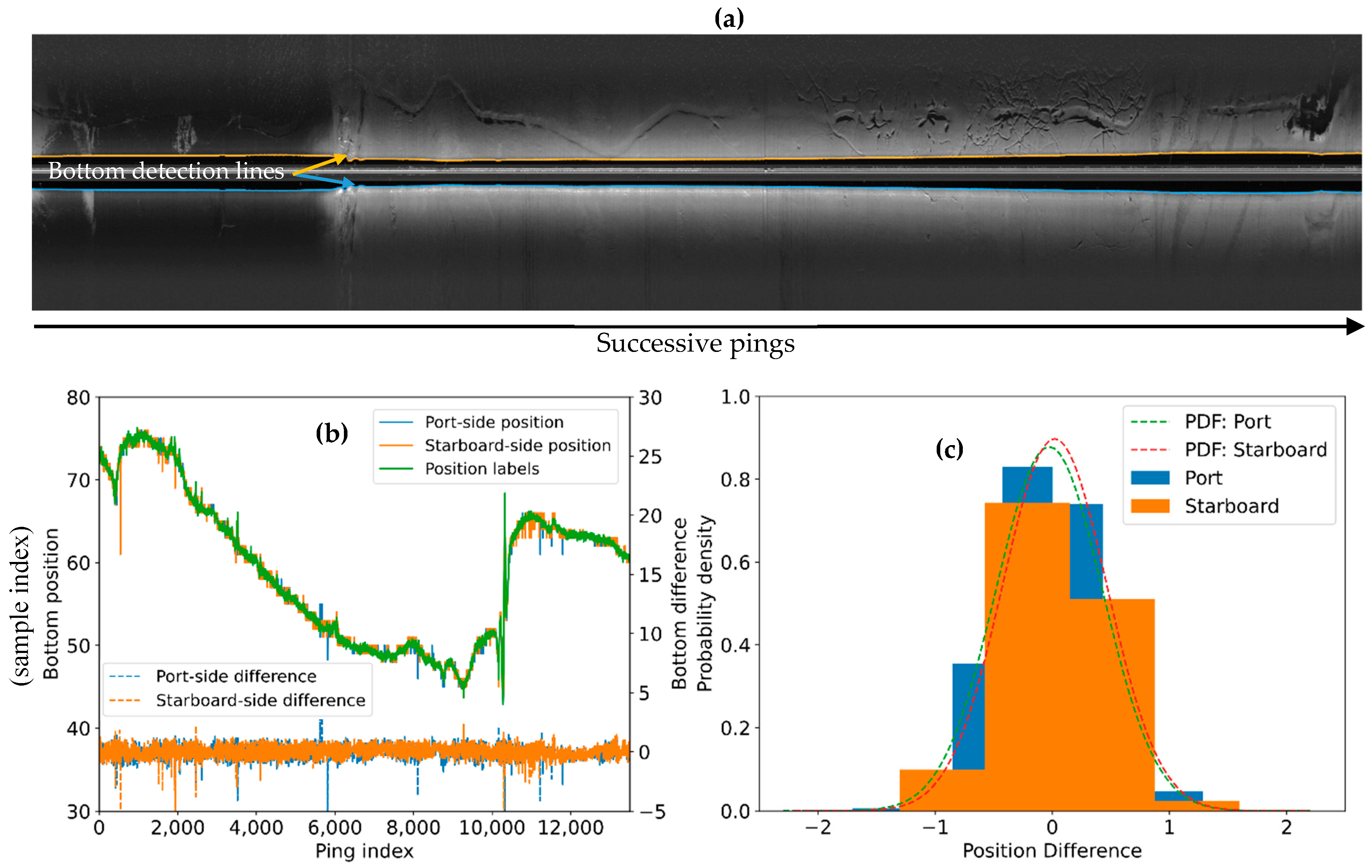
The whole side-scan data of this survey line were processed using the trained 1D-UNet model following the procedure illustrated in Figure 5 and Figure 6. The sea bottom detection results of the port-side and starboard-side side-scan data were processed and displayed on the side-scan waterfall image (Figure 10a).
In Figure 10a,b, the bottom detection results of the port-side and starboard-side pings of the same survey line are consistent with the target results. The bottom detection lines in the waterfall image (Figure 10a) also intuitively reflect the boundary between the water column and the seabed. The position (backscatter sample index) differences between the bottom detection positions of the port-side (starboard-side) pings and the targets were calculated (Figure 10b). The difference curves varied within a small range near zero. By statistical analysis, the histograms and fitted probability distribution function (PDF) curves of the port-side and starboard-side position differences are shown in Figure 10c. The main histograms are within the range of 2, which meets the correctness requirement of the position deviation less than 0.5% of the target sample length in Equation (6). The PDF curve of the port-side differences is fitted with the normal distribution curve, with the expectation μ as 0.02 and the variance σ as 0.44. The PDF curve of the starboard-side differences are also fitted with the normal distribution curve, with the expectation μ as −0.03 and the variance σ as 0.45. According to the sample number and Equation (7), the total bottom detection accuracy of the whole line is 99.88%, which proves the validity of the 1D-UNet model and the methods in this work.

3.1.2. Validation of Other Survey Lines

To further validate the 1D-UNet model and methods, the measured side-scan data of five survey lines in Meizhou Bay were randomly selected for bottom detection and tracking processing. The waterfall images of these five survey lines are shown in Figure 11.
The survey line (a) contains 4865 pings, with a maximum slant range of 84 m. Obvious sediment variation and seabed targets (pipelines) are shown in Figure 11a. Strong noises will appear near the positions where the transducer starts to record due to the sonar self-noise and vessel noise, which will influence the bottom detection results. The two long pipelines on the seabed also cause a great variation in the backscatter strength sequences. When the targets are close to the sea bottom positions, they will influence the bottom detection results.
The survey line (b) contains 5976 pings, with a maximum slant range of 84 m. Small seabed targets and seabed texture variation are shown in Figure 11b. The data measured in the same water area were all affected by sonar and vessel noises, and strong noises also appear at the center of the waterfall image. The seabed texture variation also results in variations in the side-scan backscatter strength sequences, which will also influence the bottom detection results.
The survey line (c) contains 8599 pings, with a maximum slant range of 150 m. Obvious sediment variation and seabed targets (pipelines) are demonstrated in Figure 11c. The strong noise band exists at the center of the waterfall image due to the sonar self-noise and vessel noise. Pipeline targets on the seabed also have some influence on the bottom detection results. Some ping data are missing, which will bring effects in the continuous bottom tracking.
The survey line (d) contains 1991 pings, with a maximum slant range of 84 m. The interference factors in Figure 11d include sonar self-noise, vessel noise, obvious sediment variation, and seabed texture variation. The survey line (d) contains 2308 pings, with a maximum slant range of 84 m. The interference factors in Figure 11e include sonar self-noise, vessel noise, seabed texture variation, and some missing ping data.
The side-scan data of these survey lines were processed using the 1D-UNet model and the bottom detection and tracking method proposed in this work. The seabed detection and tracking results (shown as blue and yellow curves, respectively) of each survey line are shown in Figure 11. The accurate seafloor detection and tracking results prove the validity and robustness of the method for process side-scan data affected by the interference factors, including sonar self-noise, vessel noise, sediment variation, seabed objects, seabed texture variation, and missing ping data.

3.2. Model Validation and Comparison with Other Methods

The same backscatter strength sequences were processed by the 1D-UNet model, the last peak method [26], and the 1D-CNN model [39], respectively, for result comparison. Then the real-time performance of the 1D-UNet was compared with the 1D-CNN model via statistical analysis.

3.2.1. Comparison with Other Methods

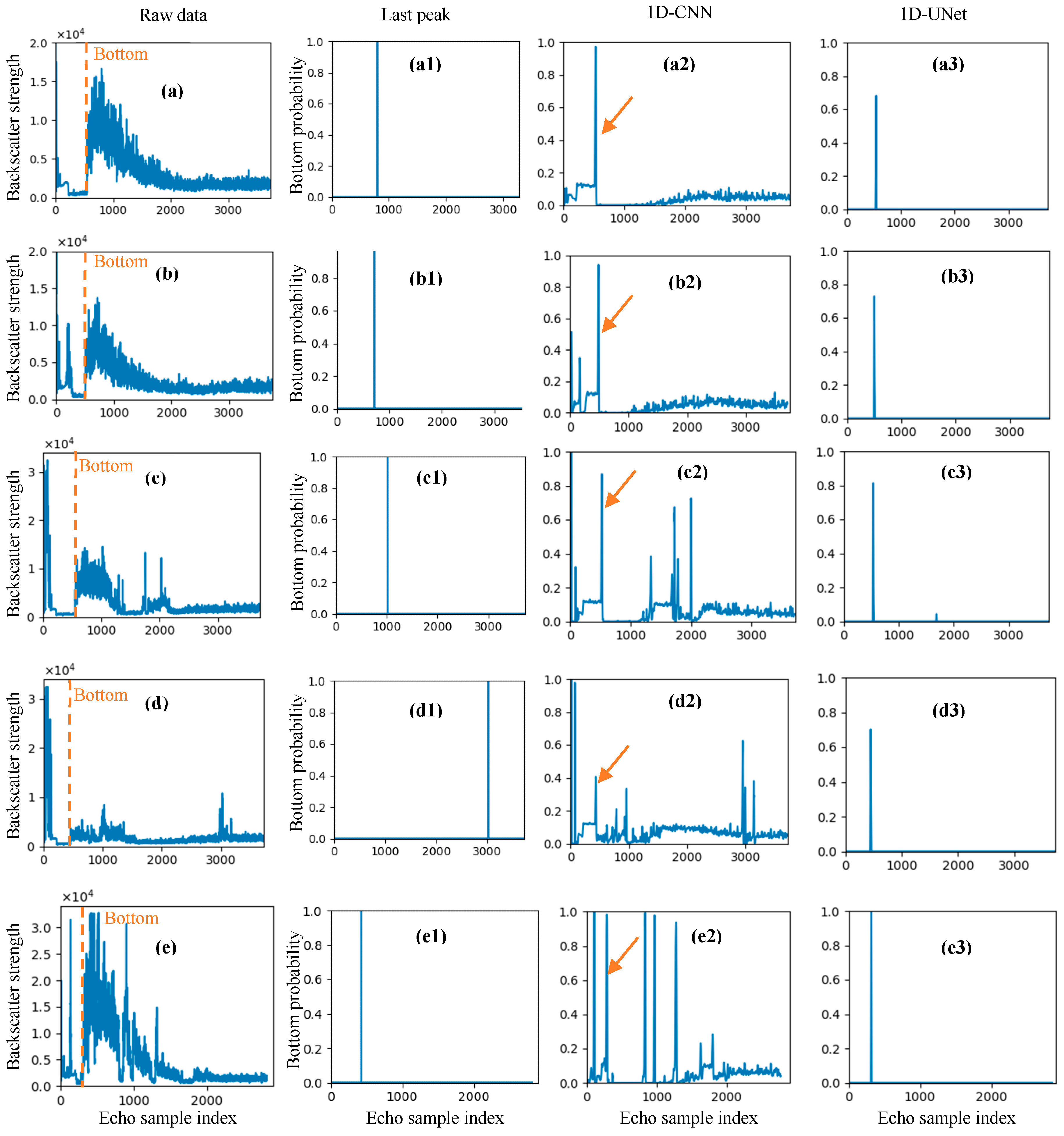
To compare the proposed method with other methods, the side-scan backscatter strength sequences of five different pings were selected and processed by using the last peak method, 1D-CNN and 1D-UNet respectively. These side-scan data were affected by different types of interference factors. The processed results are shown in Figure 12.
The five backscatter strength sequences were all compensated by unknown gains and affected by the sonar self-noise and vessel noise. No other interference factors can be observed in Figure 12a. The sequence (b) in Figure 12b was affected by suspended objects in the water column; the sequence (c) in Figure 12c was affected by seabed targets; the sequence (d) in Figure 12d was affected by the low-reflectivity sediment and high-reflectivity seabed targets; the sequence (e) in Figure 12e was affected by the suspended objects in the water column and seabed targets. To ensure comparability, the search range of all these methods is the whole backscatter strength sequence, and no other auxiliary methods were used in this experiment. The last peak method is to find the maximum strength position after removing the sonar self-noise and vessel noise. The 1D-CNN method needs to traverse the entire sequence to detect the bottom by the bottom recognition model. The 1D-UNet method directly segments the bottom from the sequence.
The last peak method is to find the maximum backscatter strength position after the sonar self-noise and vessel noise are removed. Given that the measured side-scan data were all compensated by the unknown gains, the maximum strength location is behind the location where the sound reaches the sea bottom. The detected bottom positions (Figure 12(a1,b1,c1,e1)) were all behind the true bottom position due to the combined effects of the beam patterns and gains. With regard to the backscatter strength sequence (Figure 12d) from the low-reflectivity sediment with a high-reflectivity target on the seabed, the backscatter strength from the seabed target was the maximum value, which leads to the wrong detection result (Figure 12(d1)).
The 1D-CNN method needs to traverse the entire sequence to recognize the local backscatter strength sequence at the bottom position. The bottom detection results are presented in Figure 12(a2–e2), and the real bottom positions are pointed by the arrow. In sequence (a) with less interference factors, the location with the maximum detection probability is the correct bottom location. In sequence (b), the maximum probability location is still the bottom location, although the probabilities caused by the sonar self-noise and the suspended object in the water column are high too. In sequence (c), the probability of the correct bottom position is the second largest among all the predicted probabilities. The results are mainly affected by the sonar self-noise and seabed targets. In sequence (d), the probabilities caused by the sonar self-noise and seabed targets are larger than that at the correct bottom position. In sequence (e), the probability at the correct bottom location and those caused by the suspended object in the water column and seabed targets are high. The results show that the 1D-CNN method cannot completely eliminate the effects of interference factors in the backscatter strength sequences. Thus, the search range needs to be limited to around the correct location to ensure bottom detection accuracy.
The 1D-UNet model can perceive the variation characteristics of the local and whole sequence. Accordingly, 1D-UNet shows high robustness against the interference factors, including sonar self-noise, suspended objects in the water column, seabed targets, and sediment changes. In Figure 12a3–e3, the locations of the maximum predicted probability are always the correct sea bottom location, and the probabilities caused by other interference factors are low. The comparison proves the validity and robustness of the proposed 1D-UNet model.

3.2.2. Real-time Performance and Comparison

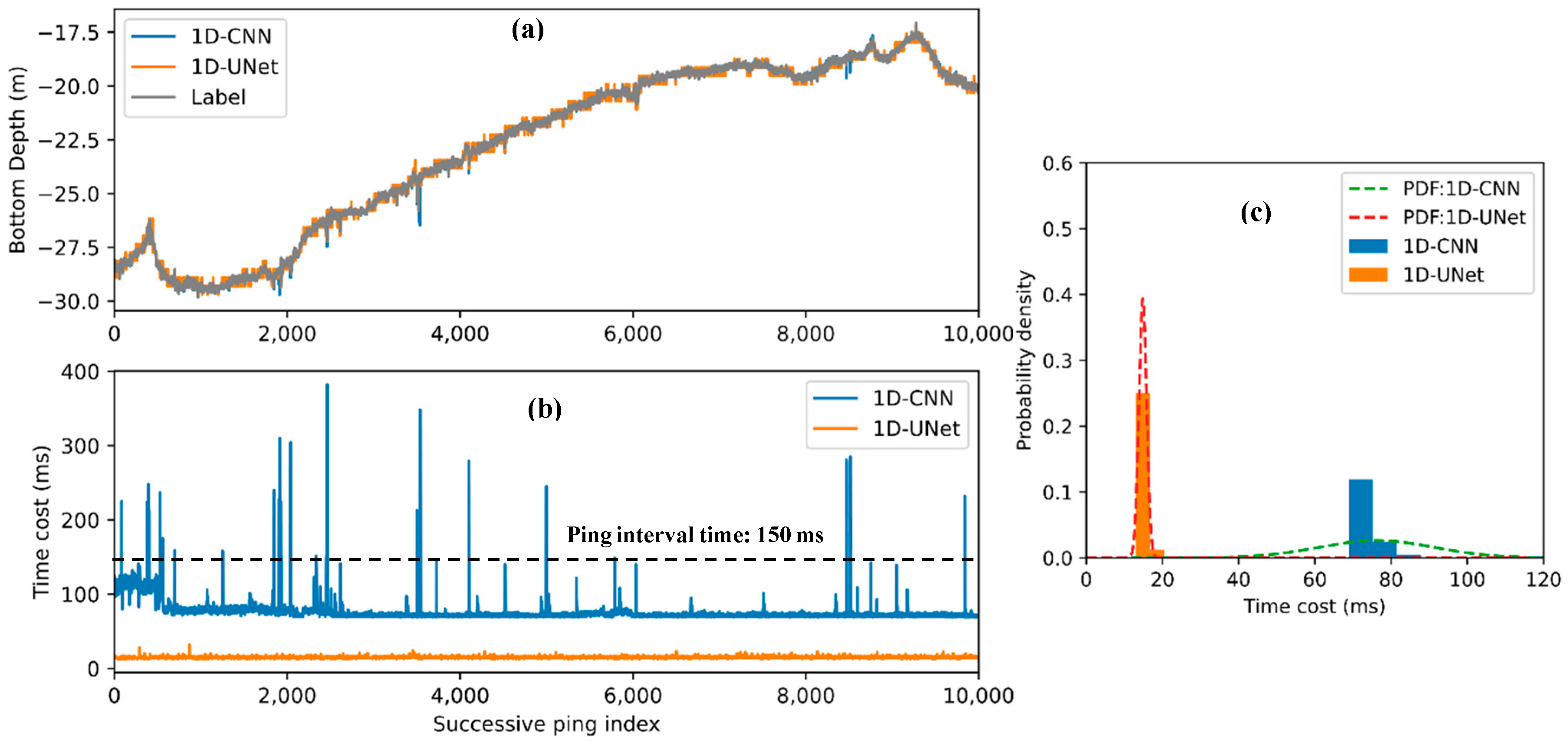
To verify and compare the real-time performance of the proposed method with the prior work, 10,000 successive ping data were processed using 1D-CNN and 1D-UNet methods. The bottom detection results of 10,000 pings are shown in Figure 13a, and the time costs of each ping are shown in Figure 13b. The time costs of each ping were statistically analyzed to evaluate the real-time performance, as shown in Figure 13c.
The 1D-CNN method uses the adaptive search range to improve the accuracy and calculation speed. In the statistical analysis, the maximum time cost of each ping is 382 ms, and the minimum time cost is 69 ms. The PDF of the time costs were fitted by a normal distribution curve with an average μ of 76.16 ms and variance σ of 15.12 ms. Considering that the ping sample interval is 150 ms, there is still more than a 0.1% chance that the time cost is larger than the ping interval when the 1D-CNN needs to search a large range, which would cause a delay in real-time processing. The time costs of the 1D-UNet method are always much lower than the ping interval time of 150 ms, with the maximum value of 32 ms and the minimum value of 13 ms. The PDF of the time costs was fitted using a normal distribution curve with μ as 14.83 ms and σ as 1.01 ms (Figure 13c). The 1D-UNet method was proven to be a fully real-time bottom detection method because the time cost of each ping by the 1D-UNet method is always shorter than the ping interval.

3.3. Bottom Detection of Side-Scan Data in Other Water Regions

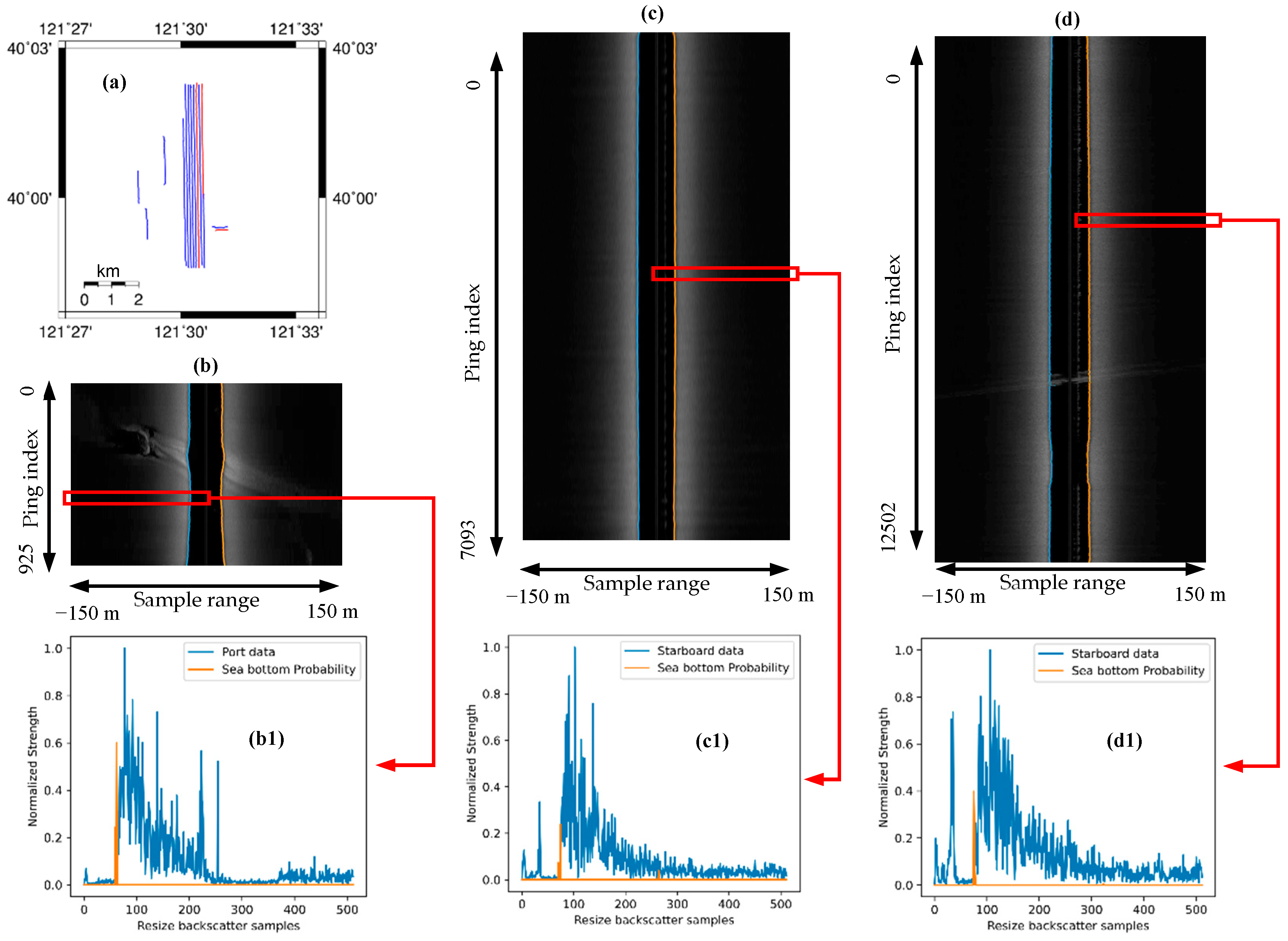
The 1D-UNet model and bottom detection and tracking method have been validated using the side-scan data measured by the same sonar model in the same water area. The measured side-scan data in the Bayuquan District were processed using the 1D-UNet model trained by the side-scan data in Meizhou Bay to further validate the generality of the proposed 1D-UNet model. The track lines of the side-scan data in the Bayuquan District are shown in Figure 14a, and three lines (in the red color) were randomly selected in this experiment.
In Figure 14, the levels of the sonar self-noise and vessel noise in the Bayuquan District were lower than those in Meizhou Bay and had lower effects on the side-scan data. The side-scan data in the Bayuquan District were also compensated by unknown time-varying gains. Figure 14 shows that the seabed sediment was quite consistent in the water region and suspended objects in the water column and some targets on the seabed are observed. The first survey line (Figure 14b) contains 925 pings, with a maximum slant range of 150 m. Some sediment variation and seabed targets are observed in Figure 14b. The second survey line (Figure 14c) contains 7093 pings, with a maximum slant range of 150 m. No obvious target was present on the seabed; however, some continuous noises are observed in the water column in Figure 14c. The third survey line contains 12,502 pings, with a maximum slant range of 150 m. Continuous noises and a large suspended object are found in the water column in Figure 14d, which would bring problems in bottom detection and tracking.
The bottom detection and tracking results of these three survey lines were processed using the 1D-UNet model trained by the side-scan data from Meizhou Bay. The bottom detection results (Figure 14b1–d1) show that the 1D-UNet can accurately detect the bottom from the side-scan data measured by various sonar models in different water regions. The experiment results proved the generality of the proposed 1D-UNet model.

4. Discussion

4.1. Advantanges of Processing Side-Scan Data in 1D Sequences

The advantages of processing 1D side-scan backscatter strength sequences rather than 2D sonar images include:
  • More samples and better accuracy. The accuracy and generality of deep learning models will improve with the increase in the number of samples. Many samples will result in higher accuracy and better generality of 1D-UNet. Considering the difficulties in marine surveys, the amount of available side-scan data is quite limited; thus, the number of 2D side-scan images will also be limited. From the perspective of 1D backscatter strength sequences, the numbers would be enormous, which would ensure the accuracy and generality of 1D-UNet.
  • Better application with lower GPU memory requirement. The 1D models need less time in training and prediction operations. The 1D convolution, pooling, and other operations are faster and require lower hardware requirements than 2D operations. With regard to integrated systems as side-scan sonars, the lower hardware requirement in the actual measurement means the lower cost and wider applications.
  • Faster speed and real-time performance. In practical side-scan sonar operation, ping data are recorded in fixed time intervals, and the real-time recorded data are the 1D backscatter strength sequences. The real-time method should be able to directly process a 1D sequence in a limited time less than the ping interval time. Therefore, the bottom detection and tracking method using 1D-UNet in this work can process side-scan data in real-time.

4.2. Other Exception Situaions

The experiment results have proved that the bottom detection and tracking method based on 1D-UNet in this work can effectively distinguish the interference factors, including unknown gain, sonar self-noise, sediment variation, suspended objects in the water column, targets on the seabed, and missing data. However, the 1D-UNet model could fail in some exceptional situations, besides these factors.
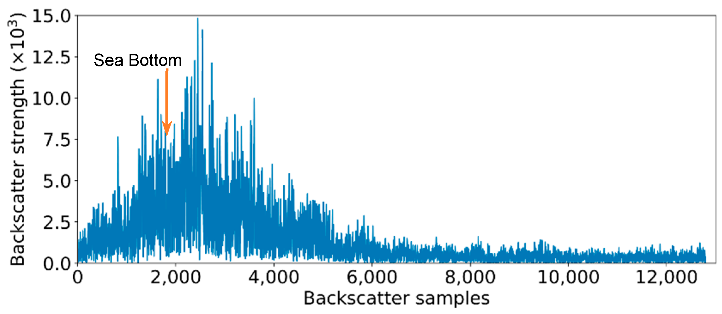
  • Very low signal to noise ratio. The 1D-UNet can detect the sea bottom position from the backscatter strength sequences in various ranges. Moreover, 1D-UNet can accurately find the bottom location as long as the backscatter strength sequences can reflect the special strength variation feature at the bottom position. However, when the signal-to-noise ratio is very low, the backscatter strength variation feature cannot be reflected in the strength sequence due to the influence of noise and other interference factors (Figure 15). In this situation, even manual labeling could also be difficult, and 1D-UNet can hardly detect the bottom location.
  • Very large suspended object. When a large suspended object is in the water column, or even almost fills the whole water column, the echo signals in the water column region could be very high. The backscatter strengths from the water column are in the same signal level as echoes from the seabed because of the high reflectivity of the suspended object and time-varying gains (Figure 16). Therefore, distinguishing the boundary between the water column and the seabed areas is difficult, and the special backscatter strength variation feature at the bottom position cannot be reflected. In this situation, neither a human being nor the 1D-UNet can easily identify the bottom location.
In these cases, the symmetry of the port-side and starboard-side data can be used. When the port-side (starboard-side) data cannot be recognized, the other-side data should be used to detect the bottom. When data on both sides cannot be recognized, the bottom position of this ping can be interpolated using the bottom positions of nearby pings based on the consistency of seabed depth variations.

4.3. Reproducibility and Application

The proposed 1D-UNet model and the bottom detection and tracking methods proposed in this paper are based on the special strength variation characteristics when the sound reaches the sea bottom. When the side-scan sonar model and operation methods are the same or similar, the 1D-UNet model trained from a part of these data can be used for the bottom detection of the other parts of these data. In the experiment, the sonar data of two water areas were measured in similar model sonars and pre-processed using similar methods. Thus, the model trained by data in Meizhou Bay can be applied to process data in the Bayuquan District. When the sonar models are quite different, or the backscatter strength sequences represent different variation characteristics, the 1D-UNet should be re-trained using the new data or updated by transfer learning to process new types of data.
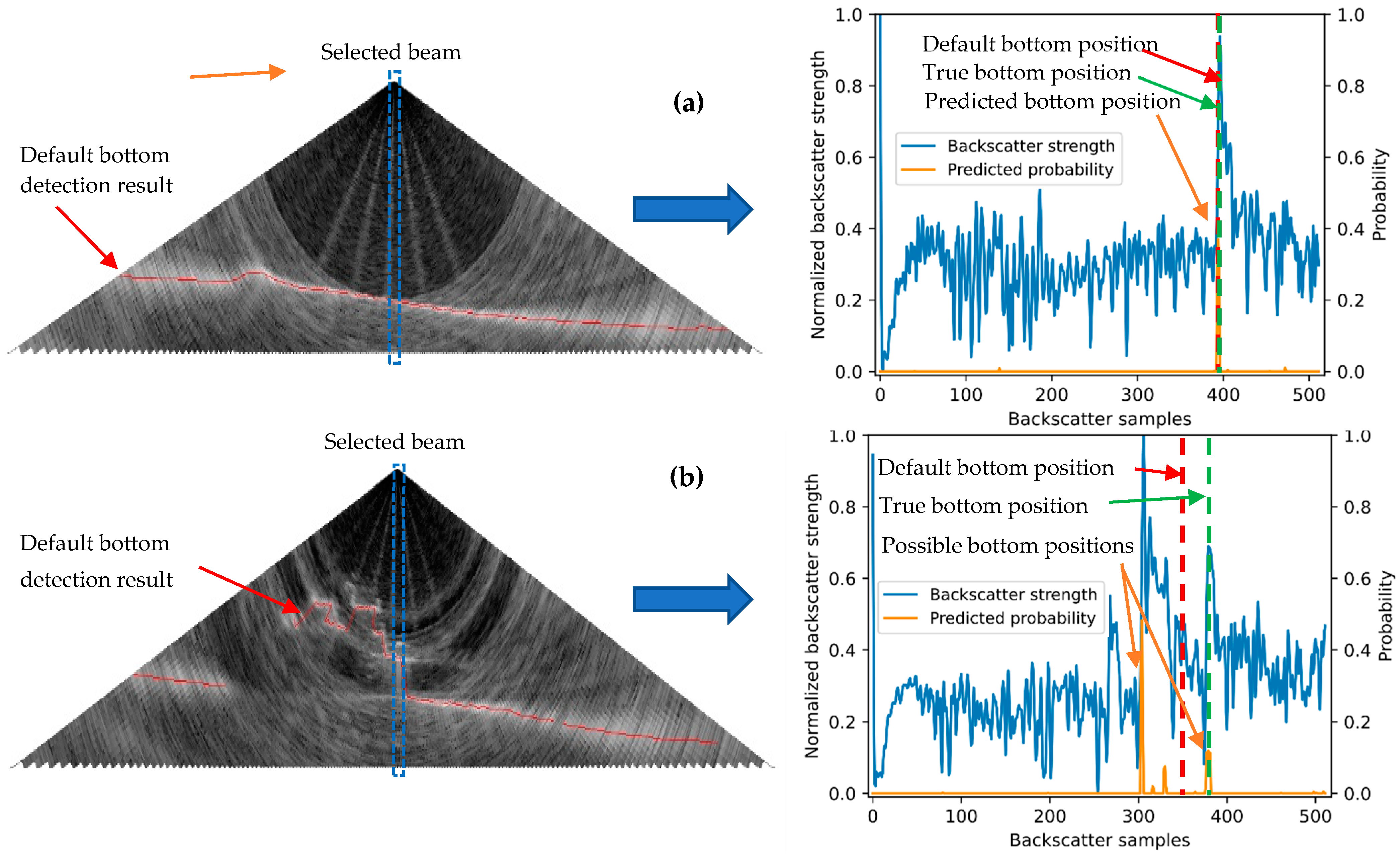
Similar to side-scan sonars, multibeam echosounders also record backscatter strengths for bottom detection, seabed, and water column imaging. Bottom detection usually is easier for multibeam echosounders, because backscatter strengths from multibeam echosounders usually are not compensated with gains and have high signal-to-noise ratios. However, when large objects (as shipwreck) lay on the seabed, traditional bottom detection methods could fail and take the shipwreck as the sea bottom (Figure 17b). To represent the potential application of 1D-UNet on multibeam echosounder, we retrained the proposed 1D-UNet model using the multibeam backscatter data measured by Kongsberg EM3002, in Swartz Bay, Canada, 2006 [45]. There existed a shipwreck on the seabed, which caused incorrect bottom detection results.
The sampling, training, and validation steps were similar to those in this work. The bottom detection results of two selected beams using the re-trained 1D-UNet model are shown in Figure 17. With no obvious objects in the water column, the bottom detection result of the selected beam (Figure 17a) obtained by the default method and 1D-UNet were both correct. While, because there existed a shipwreck in the water column in Figure 17b, the default bottom detection result was incorrect. The possible bottom positions can be obtained by 1D-UNet, and the correct position needs to be selected based on pre-known depth ranges or bottom positions of nearby beams. Moreover, the bottom detection accuracy of 1D-UNet can be improved by training with more samples. The results in Figure 17 proved the potential application of 1D-UNet on a multibeam echosounder.

5. Conclusions

A 1D-UNet model for sea bottom detection of side-scan backscatter data and the bottom detection and tracking method based on 1D-UNet are proposed in this work. The 1D-UNet model is aimed to solve the difficulties in bottom detection of the side-scan backscatter data caused by interference factors, including compensation with unknown gains, sonar self-noise, suspended objects in the water column, and seabed targets. The 1D-UNet model was first trained and validated using the side-scan data in Meizhou Bay. The training and validation accuracies were 99.92% and 99.77%, respectively, and the sea bottom detection accuracy of the training survey line was 99.88%. The model was applied to process other survey lines in Meizhou Bay and validated by the experimental results. This study compared the bottom detection results with the last peak and 1D-CNN method, and the 1D-UNet model showed better detection results and proved good robustness to the interference factors of bottom detection. In the real-time performance compassion with the 1D-CNN method, the 1D-UNet method showed better real-time performance, with a maximum time cost per ping of 32 ms, which is much less than the ping sampling interval of 150 ms. Moreover, the 1D-UNet model trained by the measured data in Meizhou Bay was applicated to process the data in the Bayuquan District. The accurate bottom detection and tracking results proved the validity and generality of the 1D-UNet model. The proposed 1D-UNet model in this work can detect the sea bottom from backscatter data of different sonars in various situations. The segmentation of the 1D sequence by using the 1D-UNet also has a certain significance for related studies.

Author Contributions

Conceptualization: J.Y. and J.M. Methodology: J.Y. Software: J.Y. Validation: J.Y., J.M. and J.Z. Formal analysis: J.Y. and J.M. Investigation: J.Y. and J.Z. Resources: J.Z. Data curation: J.Y. Writing—original draft preparation: J.Y. Writing—review and editing: J.Y., J.M. and J.Z. Visualization: J.Y. and J.M. Supervision: J.Y. and J.Z. Project administration: J.M. Funding acquisition: J.Y. and J.M. All authors have read and agreed to the published version of the manuscript.

Funding

The National Natural Science Foundation of China (grant number 41906168), Natural Science Foundation of Anhui Province (grant number 1908085QD161), and the University Natural Science Research Key Project of Anhui Province (grant number KJ2019A0024) funded this research.

Data Availability Statement

Not applicable.

Acknowledgments

The Guangzhou Marine Geological Survey Bureau provided the data in this study. The authors appreciate their support.

Conflicts of Interest

The authors declare no conflict of interest.

References

  1. Collier, J.S.; Humber, S.R. Time-lapse side-scan sonar imaging of bleached coral reefs: A case study from the Seychelles. Remote Sens. Environ. 2007, 108, 339–356. [Google Scholar] [CrossRef]
  2. Le Bas, T.P.; Huvenne, V.A.I. Acquisition and processing of backscatter data for habitat mapping—Comparison of multibeam and sidescan systems. Appl. Acoust. 2009, 70, 1248–1257. [Google Scholar] [CrossRef]
  3. Lucieer, V.L. Object-oriented classification of sidescan sonar data for mapping benthic marine habitats. Int. J. Remote Sens. 2008, 29, 905–921. [Google Scholar] [CrossRef]
  4. Yulin, T.; Jin, S.; Bian, G.; Zhang, Y. Shipwreck Target Recognition in Side-Scan Sonar Images by Improved YOLOv3 Model Based on Transfer Learning. IEEE Access 2020, 8, 173450–173460. [Google Scholar] [CrossRef]
  5. Li, J.; Jiang, P.; Zhu, H. A Local Region-Based Level Set Method With Markov Random Field for Side-Scan Sonar Image Multi-Level Segmentation. IEEE Sens. J. 2021, 21, 510–519. [Google Scholar] [CrossRef]
  6. Fakiris, E.; Zoura, D.; Ramfos, A.; Spinos, E.; Georgiou, N.; Ferentinos, G.; Papatheodorou, G. Object-based classification of sub-bottom profiling data for benthic habitat mapping. Comparison with sidescan and RoxAnn in a Greek shallow-water habitat. Estuar. Coast. Shelf Sci. 2018, 208, 219–234. [Google Scholar] [CrossRef]
  7. Trzcinska, K.; Janowski, L.; Nowak, J.; Rucinska-Zjadacz, M.; Kruss, A.; von Deimling, J.S.; Pocwiardowski, P.; Tegowski, J. Spectral features of dual-frequency multibeam echosounder data for benthic habitat mapping. Mar. Geol. 2020, 427, 106239. [Google Scholar] [CrossRef]
  8. Galvez, D.S.; Papenmeier, S.; Hass, H.C.; Bartholomae, A.; Fofonova, V.; Wiltshire, K.H. Detecting shifts of submarine sediment boundaries using side-scan mosaics and GIS analyses. Mar. Geol. 2020, 430, 106343. [Google Scholar] [CrossRef]
  9. Isachenko, A.; Gubanova, Y.; Tzetlin, A.; Mokievsky, V. High-resolution habitat mapping on mud fields: New approach to quantitative mapping of Ocean quahog. Mar. Environ. Res. 2014, 102, 36–42. [Google Scholar] [CrossRef]
  10. Cui, X.; Liu, H.; Fan, M.; Ai, B.; Ma, D.; Yang, F. Seafloor habitat mapping using multibeam bathymetric and backscatter intensity multi-features SVM classification framework. Appl. Acoust. 2021, 174, 107728. [Google Scholar] [CrossRef]
  11. Acosta, G.G.; Villar, S.A. Accumulated CA–CFAR Process in 2-D for Online Object Detection From Sidescan Sonar Data. IEEE J. Ocean. Eng. 2015, 40, 558–569. [Google Scholar] [CrossRef]
  12. Reed, S.; Petillot, Y.; Bell, J. An automatic approach to the detection and extraction of mine features in sidescan sonar. IEEE J. Ocean. Eng. 2003, 28, 90–105. [Google Scholar] [CrossRef]
  13. Blondel, P. Automatic mine detection by textural analysis of COTS sidescan sonar imagery. Int. J. Remote Sens. 2000, 21, 3115–3128. [Google Scholar] [CrossRef]
  14. Huo, G.; Yang, S.X.; Li, Q.; Zhou, Y. A Robust and Fast Method for Sidescan Sonar Image Segmentation Using Nonlocal Despeckling and Active Contour Model. IEEE Trans. Cybern. 2017, 47, 855–872. [Google Scholar] [CrossRef] [PubMed]
  15. Zhu, B.; Wang, X.; Chu, Z.; Yang, Y.; Shi, J. Active Learning for Recognition of Shipwreck Target in Side-Scan Sonar Image. Remote Sens. 2019, 11, 243. [Google Scholar] [CrossRef] [Green Version]
  16. Song, Y.; He, B.; Zhao, Y.; Li, G.; Sha, Q.; Shen, Y.; Yan, T.; Nian, R.; Lendasse, A. Segmentation of Sidescan Sonar Imagery Using Markov Random Fields and Extreme Learning Machine. IEEE J. Ocean. Eng. 2019, 44, 502–513. [Google Scholar] [CrossRef]
  17. Buscombe, D.; Grams, P.E.; Smith, S.M.C. Automated Riverbed Sediment Classification Using Low-Cost Sidescan Sonar. J. Hydraul. Eng. 2016, 142, 06015019. [Google Scholar] [CrossRef]
  18. Blomberg, A.E.A.; Sæbø, T.O.; Hansen, R.E.; Pedersen, R.B.; Austeng, A. Automatic Detection of Marine Gas Seeps Using an Interferometric Sidescan Sonar. IEEE J. Ocean. Eng. 2017, 42, 590–602. [Google Scholar] [CrossRef]
  19. Degraer, S.; Moerkerke, G.; Rabaut, M.; Van Hoey, G.; Du Four, I.; Vincx, M.; Henriet, J.-P.; Van Lancker, V. Very-high resolution side-scan sonar mapping of biogenic reefs of the tube-worm Lanice conchilega. Remote Sens. Environ. 2008, 112, 3323–3328. [Google Scholar] [CrossRef]
  20. Capus, C.G.; Banks, A.C.; Coiras, E.; Ruiz, I.T.; Smith, C.J.; Petillot, Y.R. Data correction for visualisation and classification of sidescan SONAR imagery. IET Radar Sonar Navig. 2008, 2, 155–169. [Google Scholar] [CrossRef]
  21. Reed, S.; Ruiz, I.T.; Capus, C.; Petillot, Y. The fusion of large scale classified side-scan sonar image mosaics. IEEE Trans. Image Process. 2006, 15, 2049–2060. [Google Scholar] [CrossRef] [PubMed]
  22. Capus, C.; Ruiz, I.T.; Petillot, Y. Compensation for changing beam pattern and residual tvg effects with sonar altitude variation for sidescan mosaicing and classification. In Proceedings of the 7th European Conference Underwater Acoustics, Delft, The Netherlands, 5–8 July 2004. [Google Scholar]
  23. Zhao, J.; Yan, J.; Zhang, H.; Zhang, Y.; Wang, A. A new method for weakening the combined effect of residual errors on multibeam bathymetric data. Mar. Geophys. Res. 2014, 35, 379–394. [Google Scholar] [CrossRef]
  24. Al-Rawi, M.; Elmgren, F.; Frasheri, M.; Cürüklü, B.; Yuan, X.; Martínez, J.; Bastos, J.; Rodriguez, J.; Pinto, M. Algorithms for the detection of first bottom returns and objects in the water column in sidescan sonar images. In Proceedings of the OCEANS 2017—Aberdeen, Aberdeen, UK, 19–22 June 2017; pp. 1–5. [Google Scholar]
  25. Ruiz, I.T.; Raucourt, S.D.; Petillot, Y.; Lane, D.M. Concurrent mapping and localization using sidescan sonar. IEEE J. Ocean. Eng. 2004, 29, 442–456. [Google Scholar] [CrossRef]
  26. Zhao, J.; Wang, X.; Zhang, H.; Wang, A. A Comprehensive Bottom-Tracking Method for Sidescan Sonar Image Influenced by Complicated Measuring Environment. IEEE J. Ocean. Eng. 2017, 42, 619–631. [Google Scholar] [CrossRef]
  27. Khan, M.A.; Kim, J. Toward Developing Efficient Conv-AE-Based Intrusion Detection System Using Heterogeneous Dataset. Electronics 2020, 9, 1771. [Google Scholar] [CrossRef]
  28. Cui, X.; Yang, F.; Wang, X.; Ai, B.; Luo, Y.; Ma, D. Deep learning model for seabed sediment classification based on fuzzy ranking feature optimization. Mar. Geol. 2021, 432, 106390. [Google Scholar] [CrossRef]
  29. Dirscherl, M.; Dietz, A.J.; Kneisel, C.; Kuenzer, C. A Novel Method for Automated Supraglacial Lake Mapping in Antarctica Using Sentinel-1 SAR Imagery and Deep Learning. Remote Sens. 2021, 13, 197. [Google Scholar] [CrossRef]
  30. Wang, H.; Yang, J.; Zhu, J.; Ren, L.; Liu, Y.; Li, W.; Chen, C. Estimation of Significant Wave Heights from ASCAT Scatterometer Data via Deep Learning Network. Remote Sens. 2021, 13, 195. [Google Scholar] [CrossRef]
  31. Wu, P.; Yin, Z.; Yang, H.; Wu, Y.; Ma, X. Reconstructing Geostationary Satellite Land Surface Temperature Imagery Based on a Multiscale Feature Connected Convolutional Neural Network. Remote Sens. 2019, 11, 300. [Google Scholar] [CrossRef] [Green Version]
  32. Khan, M.A.; Kim, Y. Cardiac Arrhythmia Disease Classification Using LSTM Deep Learning Approach. Comput. Mater. Contin. 2021, 67, 427–443. [Google Scholar] [CrossRef]
  33. Yuan, Q.; Shen, H.; Li, T.; Li, Z.; Li, S.; Jiang, Y.; Xu, H.; Tan, W.; Yang, Q.; Wang, J.; et al. Deep learning in environmental remote sensing: Achievements and challenges. Remote Sens. Environ. 2020, 241, 111716. [Google Scholar] [CrossRef]
  34. Xie, Y. Machine Learning for Inferring Depth from Side-Scan Sonar Images. Master’s Thesis, KTH Royal Institude of Technology, Stockholm, Sweden, September 2019. [Google Scholar]
  35. Sun, J.; Xu, G.; Ren, W.; Yan, Z. Radar emitter classification based on unidimensional convolutional neural network. IET Radar Sonar Navig. 2018, 12, 862–867. [Google Scholar] [CrossRef]
  36. Abdeljaber, O.; Avci, O.; Kiranyaz, S.; Gabbouj, M.; Inman, D. Real-Time Vibration-Based Structural Damage Detection Using One-Dimensional Convolutional Neural Networks. J. Sound Vib. 2017, 388, 154–170. [Google Scholar] [CrossRef]
  37. Milletari, F.; Navab, N.; Ahmadi, S.A. V-Net: Fully Convolutional Neural Networks for Volumetric Medical Image Segmentation. In Proceedings of the 2016 Fourth International Conference on 3D Vision (3DV), Stanford, CA, USA, 25–28 October 2016. [Google Scholar]
  38. Isensee, F.; Petersen, J.; Klein, A.; Zimmerer, D.; Jaeger, P.F.; Kohl, S.; Wasserthal, J.; Koehler, G.; Norajitra, T.; Wirkert, S.; et al. Abstract: nnU-Net: Self-adapting Framework for U-Net-Based Medical Image Segmentation. In Proceedings of the Bildver-Arbeitung für die Medizin 2019, Wiesbaden, Germany, 17–19 March 2019. [Google Scholar]
  39. Yan, J.; Meng, J.; Zhao, J. Real-Time Bottom Tracking Using Side Scan Sonar Data Through One-Dimensional Convolutional Neural Networks. Remote Sens. 2020, 12, 37. [Google Scholar] [CrossRef] [Green Version]
  40. Ronneberger, O.; Fischer, P.; Brox, T. U-Net: Convolutional Networks for Biomedical Image Segmentation. In Proceedings of the Medical Image Computing and Computer-Assisted Intervention—MICCAI 2015, Munich, Germany, 5–9 October 2015. [Google Scholar]
  41. Wang, Q.; Wu, M.; Yu, F.; Feng, C.; Li, K.; Zhu, Y.; Rigall, E.; He, B. RT-Seg: A Real-Time Semantic Segmentation Network for Side-Scan Sonar Images. Sensors 2019, 19, 1985. [Google Scholar] [CrossRef] [PubMed] [Green Version]
  42. Dmitrieva, M.; Lefebvre, J.; Peñas, K.D.; Zenner, H.L.; Richens, J.; Johnston, D.S.; Rittscher, J. Short Trajectory Segmentation with 1D UNET Framework: Application to Secretory Vesicle Dynamics. In Proceedings of the 2020 IEEE 17th International Symposium on Biomedical Imaging (ISBI), Iowa City, IA, USA, 3–7 April 2020; pp. 891–894. [Google Scholar]
  43. Shelhamer, E.; Long, J.; Darrell, T. Fully Convolutional Networks for Semantic Segmentation. IEEE Trans. Pattern Anal. 2017, 39, 640–651. [Google Scholar] [CrossRef] [PubMed]
  44. Li, Z.; Kamnitsas, K.; Glocker, B. Overfitting of Neural Nets Under Class Imbalance: Analysis and Improvements for Segmentation. In Proceedings of the Medical Image Computing and Computer Assisted Intervention—MICCAI 2019, Shenzhen, China, 13–17 October 2019; pp. 402–410. [Google Scholar]
  45. Hughes Clarke, J.E.; Lamplugh, M.; Czotter, K. Multibeam water column imaging: Improved wreck least-depth determination. In Proceedings of the Canadian Hydrographic Conference 2006, Halifax, NS, Canada, 6–9 June 2006. [Google Scholar]
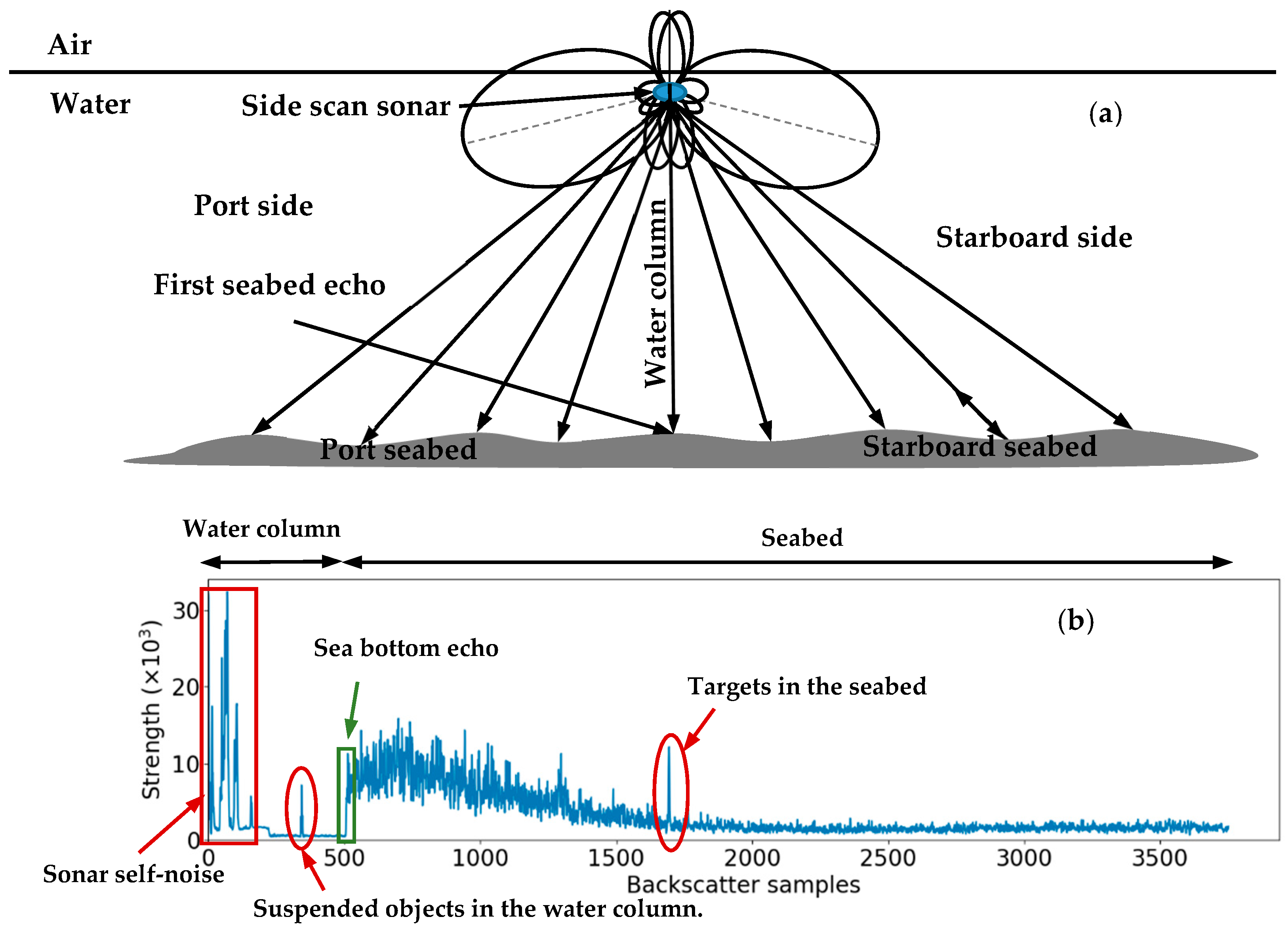
Figure 1. Operation and one-ping port-side (starboard-side) backscatter strength sequence of the side-scan sonar. (a) shows the beam pattern and the sound propagation of a side-scan sonar; (b) shows a backscatter strength sequence of a port-side (starboard-side) ping affected by many factors.
Remotesensing 13 01024 g001
Figure 2. The flow chart of the proposed one-dimensional (1D)-UNet model.
Remotesensing 13 01024 g002
Figure 3. Sampling (input and output) for the 1D-UNet model. (a) is the raw backscatter strength sequence of a ping port-side data. (b) shows normalization and resizing of the sequence. (c) shows the corresponding sea bottom probabilities of each backscatter sample.
Remotesensing 13 01024 g003
Figure 4. Structure of the proposed 1D-UNet for bottom detection from backscatter strength data of the conventional side-scan sonar.
Remotesensing 13 01024 g004
Figure 5. Bottom detection result for ping data obtained by using the trained 1D-UNet model.
Remotesensing 13 01024 g005
Figure 6. Procedure of bottom detection and tracking of successive side-scan pings.
Remotesensing 13 01024 g006
Figure 7. Experimental regions of side-scan sonar data. (a) is the Meizhou Bay region; (b) is the Bayuquan District.
Remotesensing 13 01024 g007
Figure 8. Sampling for input and target data from the measured side-scan data. (a) is the selected survey line for the training; (b) is the waterfall image constructed using the backscatter strength data; (c) shows the known sea bottom result of the survey line; (d) is the input sequence from a port-side ping data; and (e) shows the corresponding target sequence that represents the bottom probabilities.
Remotesensing 13 01024 g008
Figure 9. Training and validation accuracies and losses of 1D-UNet in 20 epochs.
Remotesensing 13 01024 g009
Figure 10. Bottom detection results obtained by using the trained 1D-UNet model. (a) shows the detected sea bottom positions of the port-side and starboard-side pings on the side-scan waterfall image; (b) shows the comparison and differences between the bottom position labels with the port-side and starboard-side predicted results; (c) shows the histograms and fitted probability distribution function (PDF) curves of the position difference data from (b).
Remotesensing 13 01024 g010
Figure 11. Sea bottom detection and tracking of other survey lines in Meizhou Bay. Panels (ae) are the corresponding bottom detection results represented on the waterfall image of five survey lines.
Remotesensing 13 01024 g011
Figure 12. Bottom detection results of five different side-scan ping data processed by the last peak method, 1D-CNN, and 1D-UNet. Panels (ae) show five different backscatter strength sequences, and i1 to i3 (i = a, b, …, e) are the detected bottom results using the last peak, 1D-CNN, and 1D-UNet, respectively.
Remotesensing 13 01024 g012
Figure 13. Real-time experimental results of 10,000 successive pings using 1D-CNN and 1D-UNet. These results were processed by the computer with AMD R5-2600X CPU and GTX-2070 GPU. (a) shows the bottom detection results of these pings; (b) shows the corresponding time costs of each ping using 1D-CNN and 1D-UNet; (c) shows the histogram and PDF curves of the time costs of 1D-CNN and 1D-UNet.
Remotesensing 13 01024 g013
Figure 14. Model validation using side-scan data in Bayuquan. (a) shows the survey track lines, and the red lines were selected for validation of the 1D-UNet model. (bd) are the bottom detection and tracking results of these three selected survey lines. (b1), (c1) and (d1) are the bottom detection result of three backscatter strength sequences from these three lines.
Remotesensing 13 01024 g014
Figure 15. Backscatter strength sequence with very low signal to noise ratio.
Remotesensing 13 01024 g015
Figure 16. Backscatter strength sequence with a very large suspended object in the water column region.
Remotesensing 13 01024 g016
Figure 17. Apply the 1D-UNet model for bottom detection from backscatter data of multibeam echosounders. (a,b) show two multibeam pings containing water column backscatter data. The backscatter strengths of selected beams in blue rectangles are processed using 1D-UNet, and the corresponding bottom detection results are obtained at the right.
Remotesensing 13 01024 g017
Publisher’s Note: MDPI stays neutral with regard to jurisdictional claims in published maps and institutional affiliations.