Abstract
Climate change increases extreme whether events such as floods, hailstorms, or storms, which can affect agriculture, causing damages and economic loss within the agro-food sector. Optical remote sensing data have been successfully used in damage detections. Cloud conditions limit their potential, especially while monitoring floods or storms that are usually related to cloudy situations. Conversely, data from the Polarimetric Synthetic Aperture Radar (PolSAR) are operational in all-weather conditions and are sensitive to the geometrical properties of crops. Apple orchards play a key role in the Italian agriculture sector, presenting a cultivation system that is very sensitive to high-wind events. In this work, the H-α-A polarimetric decomposition technique was adopted to map damaged apple orchards with reference to a stormy event that had occurred in the study area (NW Italy) on 12 August 2020. The results showed that damaged orchards have higher H (entropy) and α (alpha angle) values compared with undamaged ones taken as reference (Mann–Whitney one-tailed test U = 14,514, p < 0.001; U = 16604, p < 0.001 for H and α, respectively). By contrast, A (anisotropy) values were significantly lower for damaged orchards (Mann–Whitney one-tailed test U = 8616, p < 0.001). Based on this evidence, the authors generated a map of potentially storm-damaged orchards, assigning a probability value to each of them. This map is intended to support local funding restoration policies by insurance companies and local administrations.
1. Introduction
Climate change and related natural disasters affect several sectors [1]. Agriculture is one of the most vulnerable [2,3]. Between 2005 and 2015, the impact of natural disasters on the agricultural sector was estimated to be 96 billion dollars in damaged, or completely lost, crops [4]. Climate change-related effects (e.g., temperature and precipitation increasing in terms of level, time, and variability) are expected to reduce the yield and quality of many crops, especially cereals and fodder cereals [5].
Storms and hail also can cause serious damage to crops [6]. Hurricanes can cause much damage, with grass lodging, uprooting of orchards, and falling trees [7,8]. These critical events, potentially highly impacting farmers’ income, must be carefully accounted for in the context of risk management in agriculture.
Fruits and vegetables represent (year 2018) about 14% of the total value of European (EU) agricultural production [9,10]. These crops are very important for many EU member states, in particular for Mediterranean countries such as Spain, Italy, and France. Italy is one of the main European leaders in the apple sector [11]. Consequently, the yield loss risks concerning the fruit and vegetable sector must be minimized. Major threats concern diseases, insects, and natural disasters such as hail, drought, frost, and storms.
Apple cultivation is very intensive today, with a plant density around 2000 plants per hectare [12]. Such density allows a very high yearly production (about 45 tons per hectare) [13], which is obtained by a row-based cultivation strategy where young plants begin to be productive after the third year. The adoption of low-vigor rootstocks enables an increase in planting density and rapid fruiting. Unfortunately, this kind of cultivation determines a very underdeveloped root system, not enough to guarantee plant stability under unfavorable conditions. The situation is more critical during extreme weather events, especially when there are many weighty fruits, i.e., before harvesting [14,15]. Steel cables anchored to concrete or wooden poles are used to improve row stability.
Within this context, when a stormy event occurs, it is important to assess the spatial level and extent of damage to start remedial actions and minimize crop loss. Farmers are interested in damage estimation especially when a refund is due by insurance companies [16,17]. In this case, damage is assessed through on-the-spot checks by an expert surveyor from the insurance company, who determines the extent, type, and quality of damage. Such an approach depends on a high level of subjectivity related to the expert’s skill and experience. Moreover, these operations require a lot of time and are expensive, especially where large areas have been affected by the event.
In this operative context concerning crop damage analysis, a more objective monitoring could play a key role, providing more robust forecasts about potential yield or yield losses. Many agricultural stakeholders, such as farmers, consortia, agronomists, insurance companies, and local administrations, require a continuous monitoring of crops over large spatial extents.
A method based on free Earth Observation (EO) data can certainly represent an effective support [18] and the consequent technological transfer desirable [19,20,21,22,23,24].
In particular, optical remote sensing data have been successfully used in several operational frameworks, as proved by many works [25,26,27,28,29,30,31,32]; unfortunately, cloud conditions limit the nominal temporal resolution of this type of data, especially while monitoring natural disasters (e.g., floods or storms) that ordinarily occur when clouds are present. Data from synthetic aperture radar (SAR) systems can operate during all-weather conditions, and, while exploring agronomical issues, they can be used to analyze the moisture and geometrical conditions of crops [33,34,35]. In particular, dual-polarimetric SAR acquisitions from Copernicus Sentinel-1 mission (S1) provide unique opportunities to disseminate operational monitoring for several application communities [36,37]. Dual-pol acquisition mode has a larger swath and a lower data volume compared with full-pol acquisitions, thus improving data collection and processing for operational activities [38,39]. Polarimetric data can provide information about polarization amplitude and phase, allowing scattering mechanism definition (i.e., single-bounce, double-bounce, or volume scattering) induced by target properties. SAR polarimetry (PolSAR) is a technique that analyzes SAR polarization with respect to the vector of polarized electromagnetic waves. When a signal passes through a medium, the refraction index changes, or when it strikes an object, it is reflected; the so-called backscattering matrix [40] contains information about the reflectivity, shape, and orientation of the reflecting target. An important improvement in the extraction of physical information from the ordinary coherent backscattering matrix was achieved by Cloude and Pottier [41,42], who proposed the composition of system vectors. Most studies have assessed the sensitivity of polarimetric indicators derived from the C-band space-borne SAR to derive crop parameters [43]. The PolSAR technique was successfully applied to monitor crop growth and give estimates of yield. For example, Betberder [44] analyzed temporal trends of polarimetric indicators, proving their high potential to detect crop growth changes. Valcarce [45] used polarimetric data time series for land-cover classification, adopting a decision tree classification algorithm performing high crop class detection accuracies. Mercier and Qi [46,47] used PolSAR to support/integrate vegetation phenology monitoring based on optical data.
Only few works referring to PolSAR application in crop damage analysis are present in the literature [48,49], denoting a lack of scientific production about this issue. Nevertheless, hailstorms and storms are known to change vegetation structure, resulting in lodging or tree uprooting/breaking. Therefore, this peculiar effect changes polarimetric response and could be used to detect and characterize tree structure [50]. In general, it can be said that decomposition techniques offer a new insight into PolSAR data for describing vegetation structural proprieties [51].
The polarimetric decomposition technique decomposes the signal into its individual scattering components, permitting identification of the dominant scattering type [42,52]; this information is related to the target structural properties [18,53,54]. Various decomposition techniques have been proposed, and Lee and Cloude provided a comprehensive review about this topic [42,55]. Model-based [56] and eigenvector-based [41] algorithms have been preferred by many researchers [51]. According to Ji and his collaborators [57], the Cloude–Pottier H-α-A decomposition seems to be the most promising approach. It is based on second-order statistics extracted by a set of neighbor pixels that are used to calculate the local entropy H and the α angle (related to average scattering mechanisms). These are used to define a Cartesian space, H-α, that is linearly divided into nine zones describing the main scattering mechanisms. Recently, eigenvector decomposition has been widely applied in several applications [55,58,59,60,61]. The method was originally developed for quad-polarization data. Nevertheless, it was also adapted to work with dual-pol data [57,62,63], and consequently, it can be successfully used to retrieve polarimetric information also from S1 data that are unable to collect quad-pol data.
In this work, the applicability of the H-α-A polarimetric decomposition technique to the detection and mapping of damages from storms affecting fruit orchards was tested. In particular, the proposed case study refers to the stormy event that occurred in Northwest Italy on 12 August 2020. Consequently, a map of potentially damaged orchards was generated with the aim of supporting insurance companies and local administrations to address their funding restoration policies.
2. Materials and Methods
2.1. Study Area
On 12 August 2020, an exceptional storm affected the Northwest of Italy. In particular, the storm uprooted many apple orchards in the province of Cuneo (Piemonte region, NW Italy). Moreover, it occurred in a critical period of the year, when the main fruits (apples, pears, and peaches) were still to be harvested (Figure 1). Because in this period the farmers are focused on harvesting, no early recovery efforts were performed in the damaged fields. Therefore, the majority of the uprooted trees were not removed until October.
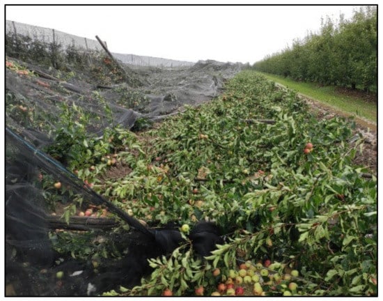
Figure 1.
An apple orchard (cultivar “Gala”) with hail nets uprooted by the storm on 12 August 2020. At the bottom, many mature apples can be noted, suggesting the economic loss caused by the storm.
The study area includes four municipalities: Saluzzo, Verzuolo, Manta, and Lagnasco (Figure 2). The area of interest (AOI) is sized about 132.23 km2. It plays a crucial economic role in Piemonte fruit production. In fact, this zone is suitable for this cultivation: the loose soil without water stagnation, sunny and dry atmosphere, and strong temperature difference between day and night allow the correct ripening and coloring of fruits. Apples represent the primary crop in Manta. Since August is a droughty period in the AOI, no significative previous precipitations had occurred before the event; 1.2 mm had cumulated in the previous week, as reported by the regional environmental agency (www.arpa.piemonte.it). Therefore, the authors supposed that moisture-related conditions cannot significantly affect the SAR signal.
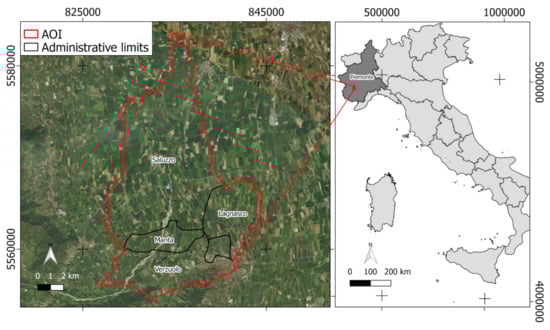
Figure 2.
Italian regions (light gray) and the Piemonte region (dark gray). (Red) The AOI includes the Saluzzo, Manta, Lagnasco, and Verzuolo municipalities (reference frame: WGS84 UTM32N).
2.2. Data and Data Collection
2.2.1. Sentinel-1 Data
Sentinel-1 is currently one of the largest space-borne missions providing free and openly accessible SAR data. The S1 mission relies on a constellation of two satellites (Sentinel-1A and Sentinel-1B) operating in the C-band (5.54 cm wavelength). The main acquisition mode over land is the Interferometric Wide (IW) swath, recording approximately 250 km in length at 5 × 20 m spatial resolution in a single look. Ordinarily, S1 records data in a dual pole mode (VV and VH), where electromagnetic waves are polarized vertically (V) for transmission and horizontally/vertically for reception. The data are recorded as complex values (I/Q components) and in SAR geometry (range and azimuth). A descending single-look complex (SLC) IW image (relative orbit no. 139), acquired after the storm (14 August 2020), was obtained from the Copernicus Open Access Hub (https://scihub.copernicus.eu/dhus/#/home, accessed: 20 December 2020).
2.2.2. Cadastral Data
A cadastral map coupled with farmers’ applications for EU Common Agricultural Policy (CAP) incentives was used in this work to classify the orchards in the AOI. The correspondent map (hereafter called orchard map (OM)) was consequently generated. The damaged orchards were analyzed at cadastral parcel level. The cadastral map was obtained for free from the regional geoportal in vector format georeferenced in the WGS84 UTM zone 32N reference frame and updated in 2018 (nominal scale was 1:2000). Databases containing farmers’ applications for EU CAP incentives of 2019 were used to map orchard types in the AOI (2020 data are not yet available). Every year, farmers support their activities with CAP incentives. These data were obtained for free from the regional public information system for agriculture. CAP applications contain the cadastral parcel code and the declaration of the most relevant crops as communicated by farmers. In this way, it is possible to couple the cadastral map with crop type information at parcel level by an ordinary join operation available in the Geographical Information System (GIS) software. In this work, 2040 (about 1136 ha) apple orchards were selected from the joined data to test the procedure.
2.2.3. Ground Dataset
A ground survey was conducted to gather the field data needed to calibrate and validate the PolSAR-based mapping procedure. In total, 72 apple orchards were surveyed (about 3.5% of the apple orchards in the AOI) during a ground campaign aimed at labeling damaged (22) and undamaged (50) fields. Specifically, the surveyed fields have an average size of about 0.92 ha, fitting well with the S1 geometrical resolution. In fact, about 40 S1 pixels can characterize each field. In particular, a visual assessment aimed at recognizing the following conditions was performed: if the majority of the trees were uprooted, the field was labeled as damaged; otherwise, it was labeled undamaged, and the related cadastral parcel was selected from the OM layer.
The dataset was split in a training (60%) and a test set (40%) by random selection from the surveyed parcels. In total, 13 damaged fields (hereafter called DTFs) and 28 undamaged ones (hereafter called UTFs) were assigned to the training set. Conversely, 10 damaged fields (hereafter called DVFs) and 21 undamaged ones (hereafter called UVFs) were assigned to the test set. The training and test set parcels are shown in Figure 3.
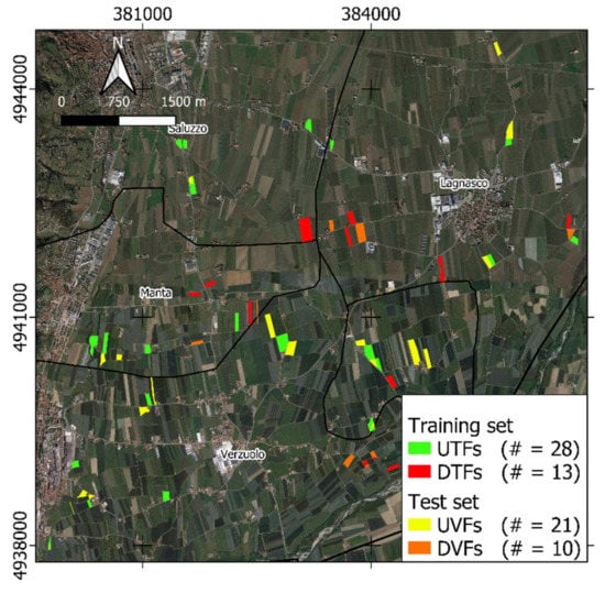
Figure 3.
Parcels belonging to the training and test sets. Colors (see legend) define the state of the surveyed parcel (damaged/undamaged). Reference frame is WGS84 UTM 32N.
This dataset was provided by local farmers. The authors found that the supplied sample includes 72 fields corresponding to about 3.5% of the apple orchards in the AOI. The authors had just the opportunity of comparing the sample size with the expected total number of apple orchards in the AOI (about 2050). The authors are aware that this sample size does not perfectly fit statical requirements. Nevertheless, it well represents ordinary availability of ground data from farmers when working with actual data not directly managed by scientists. This situation well represents a common operational condition when working with technology transfer issues, especially in the agronomic sector. In fact, the most of data from farmers, generally, rely on their autonomous collections and decision of making them public. Moreover, the private property of parcels is an objective limiting factor for all the analyses, since free access is not guaranteed. With these premises, we proceed to process the data.
A preliminary economic assessment was also performed since the storm occurred close to the apple harvesting period, determining a significant problem for local apple yield in 2020. This was obtained considering, for damaged parcels, a potential yield equal to the average one in the Piemonte region (31 t·ha−1) and a reference unitary price of 380 €·t−1. These values were obtained from the Italian Statistics Institute (ISTAT) [64].
2.3. Data Processing
2.3.1. Polarimetric Decomposition
The available S1 IW SLC image was processed to compute the polarimetric decomposition parameters. The adopted workflow is shown in Figure 4 and proposed by [65]. The target polarimetric analysis is ordinarily performed starting from the coherency matrix [66,67] or from the 2×2 covariance matrix (C2). Preprocessing steps were managed using the ESA SNAP v. 7.0.0 software [68].
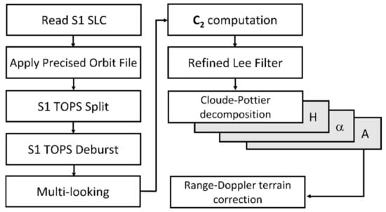
Figure 4.
The adopted workflow. All steps were managed in SNAP ESA v. 7.0.
First, the precise orbit state vector data were downloaded from the ESA archive (https://qc.sentinel1.eo.esa.int/, accessed: 20 December 2020) and applied to refine the satellite position. Precise orbit files are delivered within 20 days after data acquisition and provide accurate satellite position and velocity information. Using the TOPS split module, 1 sub-swath and 2 bursts were selected based on AOI coverage. A radiometric calibration was applied and the result saved in a complex-valued format needed to compute C2. TOPS deburst was applied by merging different bursts into a single SLC image. A spatial subset was then generated covering the AOI. The subset was multi-looked by 4 × 1 (range and azimuth direction, respectively) to generate squared pixels. The resulting multi-looked image, with a geometrical resolution equal to 15 m, was used to generate the local C2 at pixel level. With respect to quad polarization, dual-polarimetric SAR sensors generate a matrix showing the half of the totally occurring scattering components involved in fully polarimetric imagery [69]. In particular, the covariance matrix for dual polarization (e.g., Sentinel-1) is often calculated with reference to a second-order scattering information [18] generated from the spatial averaging of the scattering vector k = [SVV, SVH]T as expressed in Equation (1):
where ∗ denotes the complex conjugate and ⟨ ⟩ the local mean value in a 5 × 5 moving window. Each C2 element (C11, C22, ℜ(C12), and ℑ(C12)) is stored individually and successively refined by Lee filtering (5 × 5 kernel size) to minimize speckle-related noise. H-α-A polarimetric decomposition was obtained by eigenvector computation as proposed by different authors [57,62,63]. The modified formula for dual-pol data, as proposed by [66], is reported in Equations (2) and (3).
where λ1 ≥ λ2 ≥ 0 are the local eigenvalues, [U] is the orthogonal unitary matrix, * and T represents the complex conjugate and transpose matrices, respectively. The angles α and δ define the orientation and size of the polarization ellipse of the recorded signal [62]. The eigenvector dual-pol decomposition results in three roll-invariant parameters: polarimetric scattering entropy (H), mean scattering angle (α), and scattering anisotropy (A).
H was calculated from Equation (4):
where
H defines scatter randomness; it can vary between 0 and 1 and is related to the number of dominant scattering mechanisms, being proportional to the degree of depolarization [70]. H = 0 means that the coherency matrix shows only one eigenvalue and, therefore, the relative orientation of the correspondent pixel elements is quite simplified (e.g., single-bounce reflection).
Anisotropy A (Equation (5)) provides additional information about H in terms of the difference between scattering mechanisms.
The anisotropy quantifies the relative strength between first and second dominant scattering mechanisms. It is strictly related to the degree of signal polarization [18,71,72]. According to Mandal [18], the state of polarization of an electromagnetic (EM) wave is characterized in terms of the degree of polarization (0 ≤ A ≤ 1). The latter is defined as the ratio between the average intensity of the polarized portion of the signal and its total intensity [73]. A = 1 and A = 0 for a completely polarized and completely unpolarized wave, respectively. The unpolarized part of the received wave, (1 − A), is assumed to represent the volume scattering component from the distributed targets [74].
Average scattering mechanisms (i.e., surface, double-bounce, and volume scattering) can be identified with respect to the α parameter, which is computed according to Equation (6):
The α angles close to 0° denote a diffuse surface scattering, α close to 45° means dipole scattering (caused by volumes), and α close to 90° means double-bounce scattering mechanisms.
With these premises, the raster layer mapping local H, α, and A values was computed from the pre-processed SLC image. It was projected onto the WGS84 UTM 32N reference frame, applying the range–Doppler terrain correction. The adopted digital terrain model (DTM) needed for this step was the one freely obtainable from the Piemonte region geoportal [75]. It is supplied with a 5 m grid size and a height accuracy of ±0.30 m and was generated in 2011. The nearest-neighbor resampling method was adopted during the range–Doppler terrain correction.
2.3.2. Testing H-α-A Values after the Storm
To assess how the storm changed the orchards’ polarimetric behavior, a preliminary analysis was performed with reference to the training set. In particular, DTF and UTF pixels distributions were compared using the Mann–Whitney (MW) nonparametric test (one-tailed) [76]. The MW null hypothesis is that DTFs and UTFs have an identical distribution. The one-sided alternative “greater” was set, assuming that the DTF cumulated frequency distribution was expected to have shifted to the right of the UTF one (i.e., DTFs were greater than UTFs) [77].
The authors preliminary explored the polarimetric indices’ behavior using reference ground data. In particular, the frequency distributions were perceptively assessed using boxplots (see Section 3.1). The median value of distribution highlights a shift between damaged and undamaged fields. Therefore, to test these perceptive differences, the authors performed one tail test since the direction of changes is a priori known.
Three MW tests were performed to test if the DTF distributions of the H-α-A pixels within the parcels were statistically different from the UTF ones. All statistical analyses were performed using R software v. 3.6.3 [78]; conversely, spatial analysis was done using SAGA GIS 7.0 [79].
2.3.3. Detection of Damaged Orchards
The main goal of this work was to test the capability of the PolSAR technique to recognize damaged orchards. For this task, UTFs were assumed as representatives of the state of undamaged orchards. Samples were sized about 23 ha and represented about 2% of OM. In spite of this small sample size, the UTFs preliminarily resulted in a good dataset, whose reliability was confirmed by ground surveys. With these premises, the H-α-A distributions within UTFs were used to represent the reference distributions of the undamaged orchards. All H-α-A distributions from the AOI mapped parcels were tested against undamaged ones by the MW test, checking the following conditions: (i) parcel H distribution was greater than that of the UTFs; (ii) parcel α distribution was greater than that of the UTFs; (iii) parcel A distribution was lower than that of the UTFs. The resulting MW U-statistic and related p-value were then mapped for each orchard parcel. Moreover, the compound probability (CP) [80] was also calculated according to Equation (7) using R software v. 3.6.3. CP represents the probability that the previously mentioned three conditions were simultaneously satisfied.
where pH is the p-value resulting from the MW test under condition (i), pα is the p-value resulting from the MW test under condition (ii), and pA is the p-value resulting from the MW test under condition (iii). The resulting CP was then mapped for all OM parcels, representing its compound probability to have been damaged by the storm. A threshold value of CP able to separate damaged fields from undamaged ones has to be necessarily selected by final users, e.g., the insurance company or local public administration, according to their specific policies and strategies. Nevertheless, a possible solution is proposed here, relying on the standard error of the mean (SEM) of the CP distributions of the DTFs and UTFs. The estimated threshold value was used to generate the map of damaged orchards (DM): parcels showing a CP value lower than the threshold was classified as “undamaged,” otherwise as “damaged.” The DMs were then tested against the previously mentioned test set and the correspondent confusion matrix calculated to assess the accuracy of detection.
3. Results
3.1. H-α-A Analysis
The statistical distributions of H-α-A were computed with reference to DTFs and UTFs (Figure 5).
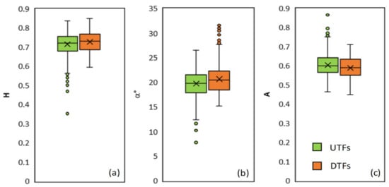
Figure 5.
Boxplots of H-α-A distributions for UTFs and DTFs. The boxplot values are from bottom to top, respectively, 5th, 25th, 50th—cross is mean value—75th, and 95th percentiles. (a) Entropy pixel distribution; (b) alpha angle pixel distribution; (c) anisotropy pixel distribution.
The MW test results (Table 1) show that the H and α distributions of DTFs presented values significantly greater than UTFs; conversely, the A distribution of the DTFs was lower than that of the UTFs.

Table 1.
MW test results obtained by comparing the H-α-A pixel distributions of DTFs and UTFs.
3.2. Damaged Orchards’ Mapping
Based on the assumption that a storm can change the polarimetric behavior of orchards according to previously mentioned dynamics, a map of CP representing the parcel probability of being recognized as damaged was generated using the UTF dataset as reference (Figure 6).
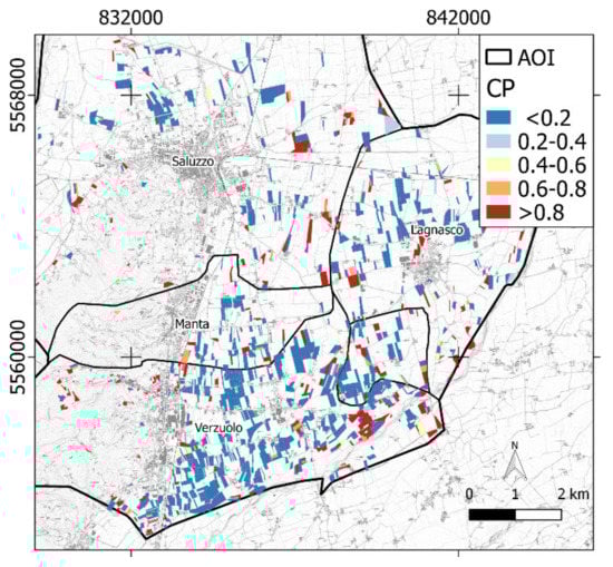
Figure 6.
A CP map of apple orchards in the AOI (Reference frame: WGS84 UTM32N).
With reference to CP, a threshold value was estimated to separate damaged fields from undamaged ones based on the SEM of CP statistic distributions of the DTFs and UTFs (Figure 7b). The DTFs showed a CP mean and SEM value of 0.715 and 0.125, respectively; consequently, one can assume that the CP mean value of all damaged orchards reasonably falls in the range 0.715 ± 0.125, about 0.6 being the lower boundary. A threshold equal to 0.6 was therefore selected to generate the DM binary classification (Figure 7a).
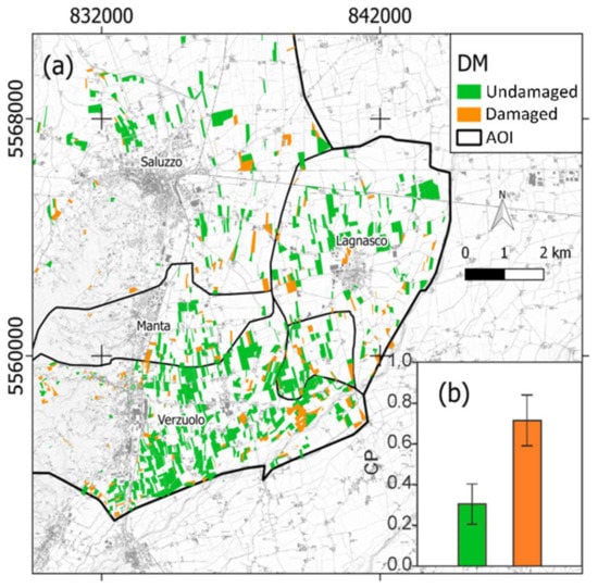
Figure 7.
(a) DM binary classification of the OM in the AOI (reference frame is WGS84 UTM 32N); (b) bar chart representing mean and 1 SEM of the CP for DTFs and UTFs.
A total of 217 ha (430 orchards) of potentially damaged apple orchards were detected in the AOI. According to the OM layer, 19% of the apple orchards were damaged after the event.
The DM was validated with respect to the test set, and the correspondent confusion matrix computed (Table 2). Classification accuracy is defined here as the one for binary classification of imbalanced data [81,82,83] since, in the test set, the number of undamaged fields was significantly greater than that of damaged fields. The resulting precision and specificity were pretty high (0.80 and 0.71, respectively), while balanced accuracy was found to be 0.75. Overall accuracy was 0.74, while F1 score (harmonic mean of the precision and recall) and G-mean (geometric mean of sensitivity and precision) were both about 0.67.
Table 2.
Metrics derived from the confusion matrix of the DM with respect to the test set. True positives (TPs): number of damaged elements predicted as damaged; false positives (FPs): number of undamaged elements predicted as damaged; false negatives (FNs): number of damaged elements predicted as undamaged; true negatives (TNs): number of undamaged elements predicted as undamaged.
Furthermore, it is worth stressing that the storm occurred close to the harvesting period, determining a significant problem for local apple yield in 2020. With reference to the AOI, a preliminary estimate of economic loss was computed to be about €2,500,000. Reported estimates could certainly vary according to the apple orchards’ age, apple variety, plant density, agronomic management, and local soil properties. Nevertheless, these estimates constituted a preliminary assessment of storm damage that occurred on 12 August 2020. Future validation is expected to test these economic deductions.
4. Discussions
Concerning the damaged orchards’ H-α-A distributions (Figure 5 and Table 1), higher values of H and α in the damaged parcels could be attributed to the changes in vegetation structure (Figure 8). In fact, the inter-row spaces of the damaged orchards, after the storm, were completely covered with the crowns of the broken or uprooted plants, which determined a different scattering geometry. Pre-event plant row geometry was characterized by a regular pattern, which drastically changed to a more disordered one, where the fallen crown elements increased the H values. Since the pre-event scattering mechanism was determined by regularly aligned and spaced plants (rows) alternating with bare soil/grass (inter-rows), it determined intermediate α values. After the storm, it can be assumed that the scattering mechanism was strongly influenced by crown volume, inducing an increase in the α values. Conversely, A appeared to reduce after the event. This could be possibly related to a reduction in the eigenvalue difference λ1 − λ2 related to the slightly different scattering mechanism after the storm. The volumetric mechanism appeared to be the prevailing one in the damaged parcels, as proved by the H increase. Since the canopy causes a strong depolarization of the SAR signal, the degree of depolarization (i.e., 1-A) tends to increase with crown closure [18]. Given these interpretation keys, the results obtained seem to support the idea that, after a relevant event able to significantly change vegetation structure, the orchards’ polarimetric behavior significantly changes. Based on the collected reference data, damaged orchards tend to show (i) higher values of H and α due to the increased contribution of the volume scattering mechanism, and (ii) lower A values, possibly due to the inter-row closure generated by broken/fallen trees, which increase signal depolarization.
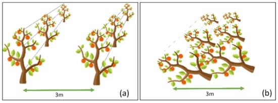
Figure 8.
A sketch representing orchard condition before (a) and after (b) the storm. In (a) the pattern row/inter-row is well defined; (b) after the storm, apple tree uprooting occurred, altering the row/inter-row pattern, and crowns covering the ground increased volumetric scattering.
Concerning the mapping of damaged orchards, the results reported in Table 2 suggest that polarimetric decomposition of S1 data is an effective approach to map orchards affected by a storm, especially during cloudy weather situations. Nevertheless, it is worth stressing that some limitations still persist while working with dual-pol decomposition. In comparison to quad polarization, dual-pol SAR sensors collect half of the scattering matrix components involved in fully polarimetric imagery. Therefore, dual-pol derived products may vary from the classical Wishart distribution. In fact, [57] highlighted that entropy/alpha decomposition using one co-polarization and one cross-polarization does not adequately extract scattering mechanisms in the H-α plane. Nevertheless, Cloude [62] proved how these differences result similarly to the conventional quad-pol one while working with vegetation. In spite of these differences, many operative frameworks were proposed proving how information lost during the dual-pol acquisition can be compensated for enhancing image swath and satellite revisit frequency. Moreover, often quad-pol SAR data are not available free of charge and not readily available for operative purposes. S1 is currently one of the largest space-borne missions providing free and open-access SAR data having high temporal resolution, fitting well with vegetation dynamics monitoring requirement.
Future developments are expected to test if pre- and post-H-α-A differences can be used to semi-automatically detect significance changes. It is worth highlighting that the majority of apple orchards in the study area are covered by plastic nets to protect the trees against hail. Probably, plastic nets can influence the complex permittivity of the analyzed volume and therefore affect the polarimetric response of the observed uprooted trees. Since in the study area, a few fields do not have hail nets, the authors did not survey such orchards, and therefore no assessment looking for the effects of nets on polarimetric response was performed. A specific research should be addressed to assess how plastic hail nets can affect backscattered signal.
5. Conclusions
In this work, a preliminary assessment about the polarimetric behavior of orchards after a storm was performed. The analysis was aimed at proposing a first methodological approach to detect orchard damage by a storm based on the PolSAR decomposition technique using S1 data. The joint adoption of free accessible S1 data, institutional free auxiliary data (a cadastral map and farmers’ CAP application database), and open software (SNAP) constituted a peculiar trait of the proposed approach. It moves in the direction of technological transfer, aiming at making SAR data/techniques an operational tool for agronomic applications, with special concern about weather-related damages to crops, which could be of interest to insurance companies or public administrations. The results proved that storm damages significantly increase the H and α parameters. By contrast, the A parameter tends to be lower in the damaged orchards. This phenomenon is possibly related to the changes affecting vegetation structure in the damaged fields, where the crowns and branches of fallen/broken plants fill the inter-row space, changing the regular pattern ordinarily characterizing apple orchards. Based on this evidence, the authors proposed a methodology to map possibly damaged orchards that relies on the knowledge about the behavior of witness (and neighboring) undamaged orchards. The method permitted the mapping of the probability that an orchard is damaged or not, constituting a new free tool able to improve orchard monitoring after a calamitous event by regional agencies and insurance companies. It is worth reminding that only apple orchards were considered for this case study. Future developments are expected to test the effectiveness of this method in other orchard types, as pear or peach, which are very diffuse in the AOI.
Author Contributions
Conceptualization, S.D.P.; data curation, S.D.P.; formal analysis, S.D.P. and F.S.; investigation, E.B.-M.; methodology, S.D.P. and E.B.-M.; software, S.D.P.; validation, M.G.; visualization, F.S.; writing—original draft, S.D.P., F.S. and M.G.; writing—review and editing, E.T. and E.B.-M. All authors have read and agreed to the published version of the manuscript.
Funding
This research received no external funding.
Institutional Review Board Statement
Not applicable.
Informed Consent Statement
Not applicable.
Data Availability Statement
Data sharing not applicable.
Acknowledgments
We would like to thank Az. Agr. Fessia Franca for having provided ground control data and fundamental operational information useful to reach the results presented in this work.
Conflicts of Interest
The authors declare no conflict of interest.
References
- Hsiang, S.; Kopp, R.; Jina, A.; Rising, J.; Delgado, M.; Mohan, S.; Rasmussen, D.J.; Muir-Wood, R.; Wilson, P.; Oppenheimer, M. Estimating Economic Damage from Climate Change in the United States. Science 2017, 356, 1362–1369. [Google Scholar] [CrossRef]
- Nelson, G.C.; Valin, H.; Sands, R.D.; Havlík, P.; Ahammad, H.; Deryng, D.; Elliott, J.; Fujimori, S.; Hasegawa, T.; Heyhoe, E. Climate Change Effects on Agriculture: Economic Responses to Biophysical Shocks. Proc. Natl. Acad. Sci. USA 2014, 111, 3274–3279. [Google Scholar] [CrossRef]
- Moore, F.C.; Baldos, U.; Hertel, T.; Diaz, D. New Science of Climate Change Impacts on Agriculture Implies Higher Social Cost of Carbon. Nat. Commun. 2017, 8, 1–9. [Google Scholar] [CrossRef]
- FAO The Impact of Natural Hazards and Disasters on Agriculture and Food Security and Nutrition–A Call for Action to Build Resilient Livelihoods. Available online: http://www.fao.org/emergencies/resources/documents/resources-detail/zh/c/280784/ (accessed on 20 December 2020).
- Welbergen, J.A.; Klose, S.M.; Markus, N.; Eby, P. Climate Change and the Effects of Temperature Extremes on Australian Flying-Foxes. Proc. R. Soc. B. Biol. Sci. 2008, 275, 419–425. [Google Scholar] [CrossRef]
- Wang, E.; Bertis, B.L.; Jimmy, R.W.; Yu, Y. Simulation of Hail Effects on Crop Yield Losses for Corn-Belt States in USA. Trans. Chin. Soc. Agric. Eng. 2012, 28, 177–185. [Google Scholar]
- Reighard, G.L.; Parker, M.L.; Krewer, G.W.; Beckman, T.G.; Wood, B.W.; Smith, J.E.; Whiddon, J. Impact of Hurricanes on Peach and Pecan Orchards in the Southeastern United States. HortScience 2001, 36, 250–252. [Google Scholar] [CrossRef]
- Crane, J.; Balerdi, C.; Campbell, R.; Campbell, C.; Goldweber, S. Managing Fruit Orchards to Minimize Hurricane Damage. HortTechnology 1994, 4, 21–27. [Google Scholar] [CrossRef]
- Notarnicola, B.; Tassielli, G.; Renzulli, P.A.; Castellani, V.; Sala, S. Environmental Impacts of Food Consumption in Europe. J. Clean. Prod. 2017, 140, 753–765. [Google Scholar] [CrossRef]
- Bos-Brouwers, H.E.J.; Graf, V.; Aramyan, L.; Oberc, B. Food Redistribution in the EU–Mapping and Analysis of Existing Regulatory and Policy Measures Impacting Food Redistribution from EU Member States. Available online: https://research.wur.nl/en/publications/food-redistribution-in-the-eu-mapping-and-analysis-of-existing-re (accessed on 20 December 2020).
- FAO FAOSTAT. Available online: http://www.fao.org/faostat/en/#home (accessed on 13 November 2020).
- Eccher, T.; Granelli, G. Fruit Quality and Yield of Different Apple Cultivars as Affected by Tree Density. Acta Hortic. 2006, 535–540. [Google Scholar] [CrossRef]
- Childers, N.F.; Morris, J.R.; Sibbett, G.S. Modern Fruit Science: Orchard and Small Fruit Culture; Horticultural Publications: Gainesville, GA, USA, 1995. [Google Scholar]
- Lordan, J.; Gomez, M.; Francescatto, P.; Robinson, T.L. Long-Term Effects of Tree Density and Tree Shape on Apple Orchard Performance, a 20 Year Study–Part 2, Economic Analysis. Sci. Hortic. 2019, 244, 435–444. [Google Scholar] [CrossRef]
- Lauri, P. Apple Tree Architecture and Cultivation-a Tree in a System. In Proceedings of the I International Apple Symposium 1261; ISHS Acta Horticulturae: Yangling, China, 2016; pp. 173–184. [Google Scholar]
- Prabhakar, M.; Gopinath, K.A.; Reddy, A.G.K.; Thirupathi, M.; Rao, C.S. Mapping Hailstorm Damaged Crop Area Using Multispectral Satellite Data. Egypt. J. Remote Sens. Space Sci. 2019, 22, 73–79. [Google Scholar] [CrossRef]
- Botzen, W.J.W.; Bouwer, L.M.; Van den Bergh, J. Climate Change and Hailstorm Damage: Empirical Evidence and Implications for Agriculture and Insurance. Resour. Energy Econ. 2010, 32, 341–362. [Google Scholar] [CrossRef]
- Mandal, D.; Kumar, V.; Ratha, D.; Dey, S.; Bhattacharya, A.; Lopez-Sanchez, J.M.; McNairn, H.; Rao, Y.S. Dual Polarimetric Radar Vegetation Index for Crop Growth Monitoring Using Sentinel-1 SAR Data. Remote Sens. Environ. 2020, 247, 111954. [Google Scholar] [CrossRef]
- De Petris, S.; Berretti, R.; Guiot, E.; Giannetti, F.; Motta, R.; Borgogno-Mondino, E. Detection And Characterization of Forest Harvesting In Piedmont Through Sentinel-2 Imagery: A Methodological Proposal. Ann. Silvic. Res. 2020, 45, 92–98. [Google Scholar] [CrossRef]
- Sarvia, F.; De Petris, S.; Borgogno-Mondino, E. Remotely sensed data to support insurance strategies in agriculture. In Remote Sensing for Agriculture, Ecosystems, and Hydrology XXI; SPIE-Intl. Soc. Opt. Eng.: Strasbourg, France, 2019. [Google Scholar]
- Sarvia, F.; De Petris, S.; Borgogno-Mondino, E. Multi-Scale Remote Sensing to Support Insurance Policies in Agriculture: From Mid-Term to Instantaneous Deductions. GIScience Remote Sens. 2020, 57, 770–784. [Google Scholar] [CrossRef]
- Borgogno-Mondino, E.; Sarvia, F.; Gomarasca, M.A. Supporting Insurance Strategies in Agriculture by Remote Sensing: A Possible Approach at Regional Level. In Proceedings of the Lecture Notes in Computer Science; Springer Science and Business Media LLC: Berlin/Heidelberg, Germany, 2019; pp. 186–199. [Google Scholar]
- Sarvia, F.; De Petris, S.; Borgogno-Mondino, E. A Methodological Proposal to Support Estimation of Damages from Hailstorms Based on Copernicus Sentinel 2 Data Times Series. In Proceedings of the International Conference on Computational Science and Its Applications; Springer: Berlin/Heidelberg, Germany, 2020; pp. 737–751. [Google Scholar]
- Sarvia, F.; Xausa, E.; Petris, S.D.; Cantamessa, G.; Borgogno-Mondino, E. A Possible Role of Copernicus Sentinel-2 Data to Support Common Agricultural Policy Controls in Agriculture. Agronomy 2021, 11, 110. [Google Scholar] [CrossRef]
- Boryan, C.; Yang, Z.; Mueller, R.; Craig, M. Monitoring US Agriculture: The US Department of Agriculture, National Agricultural Statistics Service, Cropland Data Layer Program. Geocarto Int. 2011, 26, 341–358. [Google Scholar] [CrossRef]
- López-Lozano, R.; Duveiller, G.; Seguini, L.; Meroni, M.; García-Condado, S.; Hooker, J.; Leo, O.; Baruth, B. Towards Regional Grain Yield Forecasting with 1 Km-Resolution EO Biophysical Products: Strengths and Limitations at Pan-European Level. Agric. For. Meteorol. 2015, 206, 12–32. [Google Scholar] [CrossRef]
- Chipanshi, A.; Zhang, Y.; Kouadio, L.; Newlands, N.; Davidson, A.; Hill, H.; Warren, R.; Qian, B.; Daneshfar, B.; Bedard, F. Evaluation of the Integrated Canadian Crop Yield Forecaster (ICCYF) Model for in-Season Prediction of Crop Yield across the Canadian Agricultural Landscape. Agric. For. Meteorol. 2015, 206, 137–150. [Google Scholar] [CrossRef]
- de Wit, A.; Duveiller, G.; Defourny, P. Estimating Regional Winter Wheat Yield with WOFOST through the Assimilation of Green Area Index Retrieved from MODIS Observations. Agric. For. Meteorol. 2012, 164, 39–52. [Google Scholar] [CrossRef]
- Doraiswamy, P.C.; Sinclair, T.R.; Hollinger, S.; Akhmedov, B.; Stern, A.; Prueger, J. Application of MODIS Derived Parameters for Regional Crop Yield Assessment. Remote Sens. Environ. 2005, 97, 192–202. [Google Scholar] [CrossRef]
- Chen, Y.; Zhang, Z.; Tao, F. Improving Regional Winter Wheat Yield Estimation through Assimilation of Phenology and Leaf Area Index from Remote Sensing Data. Eur. J. Agron. 2018, 101, 163–173. [Google Scholar] [CrossRef]
- Patel, N.R.; Bhattacharjee, B.; Mohammed, A.J.; Tanupriya, B.; Saha, S.K. Remote Sensing of Regional Yield Assessment of Wheat in Haryana, India. Int. J. Remote Sens. 2006, 27, 4071–4090. [Google Scholar] [CrossRef]
- Orusa, T.; Orusa, R.; Viani, A.; Carella, E.; Borgogno Mondino, E. Geomatics and EO Data to Support Wildlife Diseases Assessment at Landscape Level: A Pilot Experience to Map Infectious Keratoconjunctivitis in Chamois and Phenological Trends in Aosta Valley (NW Italy). Remote Sens. 2020, 12, 3542. [Google Scholar] [CrossRef]
- Ulaby, F.T.; Moore, R.K.; Fung, A.K. Microwave Remote Sensing: Active and Passive. Volume 1-Microwave Remote Sensing Fundamentals and Radiometry; Artech House: Norwood, MA, USA, 1981. [Google Scholar]
- Ulaby, F. Radar Response to Vegetation. IEEE Trans. Antennas Propag. 1975, 23, 36–45. [Google Scholar] [CrossRef]
- McNairn, H.; Shang, J. A review of multitemporal synthetic aperture radar (SAR) for crop monitoring. In Multitemporal Remote Sensing; Springer: Berlin, Germany, 2016; pp. 317–340. [Google Scholar]
- Karagiannopoulou, A.; Tsiakos, C.; Tsimiklis, G.; Tsertou, A.; Amditis, A.; Milcinski, G.; Vesel, N.; Protic, D.; Kilibarda, M.; Tsakiridis, N. An integrated service-based solution addressing the modernised common agriculture policy regulations and environmental perspectives. In Proceedings Volume 11528, Remote Sensing for Agriculture, Ecosystems, and Hydrology XXII; International Society for Optics and Photonics: Bellingham, WA, USA, 2020. [Google Scholar]
- Kanjir, U.; DJurić, N.; Veljanovski, T. Sentinel-2 Based Temporal Detection of Agricultural Land Use Anomalies in Support of Common Agricultural Policy Monitoring. ISPRS Int. J. Geo Inf. 2018, 7, 405. [Google Scholar] [CrossRef]
- Lee, J.-S.; Grunes, M.R.; Pottier, E. Quantitative Comparison of Classification Capability: Fully Polarimetric versus Dual and Single-Polarization SAR. IEEE Trans. Geosci. Remote Sens. 2001, 39, 2343–2351. [Google Scholar]
- Ainsworth, T.L.; Kelly, J.P.; Lee, J.-S. Classification Comparisons between Dual-Pol, Compact Polarimetric and Quad-Pol SAR Imagery. ISPRS J. Photogramm. Remote Sens. 2009, 64, 464–471. [Google Scholar] [CrossRef]
- Boerner, W.-M.; Mott, H.; Luneburg, E. Polarimetry in Remote Sensing: Basic and Applied Concepts. In Proceedings of the IGARSS’97, 1997 IEEE International Geoscience and Remote Sensing Symposium Proceedings, Remote Sensing-A Scientific Vision for Sustainable Development Singapore, 3–8 August 1997; Volume 3, pp. 1401–1403. [Google Scholar]
- Cloude, S.R.; Pottier, E. An Entropy Based Classification Scheme for Land Applications of Polarimetric SAR. IEEE Trans. Geosci. Remote Sens. 1997, 35, 68–78. [Google Scholar] [CrossRef]
- Cloude, S.R.; Pottier, E. A Review of Target Decomposition Theorems in Radar Polarimetry. IEEE Trans. Geosci. Remote Sens. 1996, 34, 498–518. [Google Scholar] [CrossRef]
- Nasirzadehdizaji, R.; Balik Sanli, F.; Abdikan, S.; Cakir, Z.; Sekertekin, A.; Ustuner, M. Sensitivity Analysis of Multi-Temporal Sentinel-1 SAR Parameters to Crop Height and Canopy Coverage. Appl. Sci. 2019, 9, 655. [Google Scholar] [CrossRef]
- Betbeder, J.; Fieuzal, R.; Philippets, Y.; Ferro-Famil, L.; Baup, F. Contribution of Multitemporal Polarimetric Synthetic Aperture Radar Data for Monitoring Winter Wheat and Rapeseed Crops. J. Appl. Remote Sens. 2016, 10, 026020. [Google Scholar] [CrossRef]
- Valcarce-Diñeiro, R.; Arias-Pérez, B.; Lopez-Sanchez, J.M.; Sánchez, N. Multi-Temporal Dual-and Quad-Polarimetric Synthetic Aperture Radar Data for Crop-Type Mapping. Remote Sens. 2019, 11, 1518. [Google Scholar] [CrossRef]
- Mercier, A.; Betbeder, J.; Baudry, J.; Le Roux, V.; Spicher, F.; Lacoux, J.; Roger, D.; Hubert-Moy, L. Evaluation of Sentinel-1 & 2 Time Series for Predicting Wheat and Rapeseed Phenological Stages. ISPRS J. Photogramm. Remote Sens. 2020, 163, 231–256. [Google Scholar]
- Qi, Z.; Yeh, A.G.-O.; Li, X. A Crop Phenology Knowledge-Based Approach for Monthly Monitoring of Construction Land Expansion Using Polarimetric Synthetic Aperture Radar Imagery. ISPRS J. Photogramm. Remote Sens. 2017, 133, 1–17. [Google Scholar] [CrossRef]
- Zhao, L.; Yang, J.; Li, P.; Shi, L.; Zhang, L. Characterizing Lodging Damage in Wheat and Canola Using Radarsat-2 Polarimetric SAR Data. Remote Sens. Lett. 2017, 8, 667–675. [Google Scholar] [CrossRef]
- Yang, H.; Chen, E.; Li, Z.; Zhao, C.; Yang, G.; Pignatti, S.; Casa, R.; Zhao, L. Wheat Lodging Monitoring Using Polarimetric Index from RADARSAT-2 Data. Int. J. Appl. Earth Obs. Geoinf. 2015, 34, 157–166. [Google Scholar] [CrossRef]
- Dickinson, C.; Siqueira, P.; Clewley, D.; Lucas, R. Classification of Forest Composition Using Polarimetric Decomposition in Multiple Landscapes. Remote Sens. Environ. 2013, 131, 206–214. [Google Scholar] [CrossRef]
- Trisasongko, B.H. The Use of Polarimetric SAR Data for Forest Disturbance Monitoring. Sens. Imaging 2010, 11, 1–13. [Google Scholar] [CrossRef]
- Le Toan, T.; Beaudoin, A.; Riom, J.; Guyon, D. Relating Forest Biomass to SAR Data. IEEE Trans. Geosci. Remote Sens. 1992, 30, 403–411. [Google Scholar] [CrossRef]
- Ruiz, J.S.; Ordonez, Y.F.; McNairn, H. Corn Monitoring and Crop Yield Using Optical and Microwave Remote Sensing. Geosci. Remote Sens. 2008, 10, 405–420. [Google Scholar]
- Mandal, D.; Kumar, V.; Lopez-Sanchez, J.M.; Bhattacharya, A.; McNairn, H.; Rao, Y.S. Crop Biophysical Parameter Retrieval from Sentinel-1 SAR Data with a Multi-Target Inversion of Water Cloud Model. Int. J. Remote Sens. 2020, 41, 5503–5524. [Google Scholar] [CrossRef]
- Lee, J.-S.; Grunes, M.R.; Ainsworth, T.L.; Du, L.-J.; Schuler, D.L.; Cloude, S.R. Unsupervised Classification Using Polarimetric Decomposition and the Complex Wishart Classifier. IEEE Trans. Geosci. Remote Sens. 1999, 37, 2249–2258. [Google Scholar]
- Freeman, A.; Durden, S.L. A Three-Component Scattering Model for Polarimetric SAR Data. IEEE Trans. Geosci. Remote Sens. 1998, 36, 963–973. [Google Scholar] [CrossRef]
- Ji, K.; Wu, Y. Scattering Mechanism Extraction by a Modified Cloude-Pottier Decomposition for Dual Polarization SAR. Remote Sens. 2015, 7, 7447. [Google Scholar] [CrossRef]
- McNairn, H.; Shang, J.; Jiao, X.; Champagne, C. The Contribution of ALOS PALSAR Multipolarization and Polarimetric Data to Crop Classification. IEEE Trans. Geosci. Remote Sens. 2009, 47, 3981–3992. [Google Scholar] [CrossRef]
- Lopez-Sanchez, J.M.; Cloude, S.R.; Ballester-Berman, J.D. Rice Phenology Monitoring by Means of SAR Polarimetry at X-Band. IEEE Trans. Geosci. Remote Sens. 2011, 50, 2695–2709. [Google Scholar] [CrossRef]
- Ramsey III, E.; Rangoonwala, A.; Suzuoki, Y.; Jones, C.E. Oil Detection in a Coastal Marsh with Polarimetric Synthetic Aperture Radar (SAR). Remote Sens. 2011, 3, 2630. [Google Scholar] [CrossRef]
- Yonezawa, C.; Watanabe, M.; Saito, G. Polarimetric Decomposition Analysis of ALOS PALSAR Observation Data before and after a Landslide Event. Remote Sens. 2012, 4, 2314. [Google Scholar] [CrossRef]
- Cloude, S.R. The Dual Polarisation Entropy/Alpha Decomposition. In Proceedings of the 3rd International Workshop on Science and Applications of SAR Polarimetry and Polarimetric Interferometry, Noordwijk, The Netherlands; 2007; pp. 22–26. [Google Scholar]
- Ghods, S.; Shojaedini, S.V.; Maghsoudi, Y. A Modified H- α Classification Method for Dcp Compact Polarimetric Mode by Reconstructing Quad h and α Parameters from Dual Ones. IEEE J. Sel. Top. Appl. Earth Obs. Remote Sens. 2016, 9, 2233–2241. [Google Scholar] [CrossRef]
- ISTAT ISTAT Data. Available online: http://dati.istat.it/ (accessed on 13 November 2020).
- Mandal, D.; Vaka, D.S.; Bhogapurapu, N.R.; Vanama, V.S.K.; Kumar, V.; Rao, Y.S.; Bhattacharya, A. Sentinel-1 SLC Preprocessing Workflow for Polarimetric Applications: A Generic Practice for Generating Dual-Pol Covariance Matrix Elements in SNAP S-1 Toolbox. 2019. Available online: https://www.preprints.org/manuscript/201911.0393/v1 (accessed on 9 February 2021).
- Lee, J.-S.; Pottier, E. Polarimetric Radar Imaging: From Basics to Applications; CRC Press: Boca Raton, FL, USA, 2017. [Google Scholar]
- Shan, Z.; Wang, C.; Zhang, H.; Chen, J. H-Alpha Decomposition and Alternative Parameters for Dual Polarization SAR Data. In Proceedings of the PIERS Proceedings, SuZhou, China, 12–16 September 2011. [Google Scholar]
- Veci, L.; Prats-Iraola, P.; Scheiber, R.; Collard, F.; Fomferra, N.; Engdahl, M. The Sentinel-1 Toolbox. In Proceedings of the IEEE International Geoscience and Remote Sensing Symposium (IGARSS), Quebec City, QC, Canada, 13–18 July 2014; pp. 1–3. [Google Scholar]
- Ainsworth, T.L.; Kelly, J.; Lee, J.-S. Polarimetric Analysis of Dual Polarimetric SAR Imagery. In Proceedings of the 7th European Conference on Synthetic Aperture Radar; VDE, Friedrichshafen, Germany, 2–5 June 2008; 2008; pp. 1–4. [Google Scholar]
- Crabbe, R.A.; Lamb, D.W.; Edwards, C.; Andersson, K.; Schneider, D. A Preliminary Investigation of the Potential of Sentinel-1 Radar to Estimate Pasture Biomass in a Grazed Pasture Landscape. Remote Sens. 2019, 11, 872. [Google Scholar] [CrossRef]
- Chang, J.; Shoshany, M. Radar Polarization and Ecological Pattern Properties across Mediterranean-to-Arid Transition Zone. Remote Sens. Environ. 2017, 200, 368–377. [Google Scholar] [CrossRef]
- Chang, J.G.; Shoshany, M.; Oh, Y. Polarimetric Radar Vegetation Index for Biomass Estimation in Desert Fringe Ecosystems. IEEE Trans. Geosci. Remote Sens. 2018, 56, 7102–7108. [Google Scholar] [CrossRef]
- Cloude, S. Polarisation: Applications in Remote Sensing; Oxford University Press: Oxford, UK, 2009. [Google Scholar]
- Raney, R.K.; Cahill, J.T.; Patterson, G.W.; Bussey, D.B.J. The M-Chi Decomposition of Hybrid Dual-Polarimetric Radar Data with Application to Lunar Craters. J. Geophys. Res. Planets 2012, 117. [Google Scholar] [CrossRef]
- Borgogno Mondino, E.; Fissore, V.; Lessio, A.; Motta, R. Are the New Gridded DSM/DTMs of the Piemonte Region (Italy) Proper for Forestry? A Fast and Simple Approach for a Posteriori Metric Assessment. iFor. Biogeosci. For. 2016, 9, 901–909. [Google Scholar] [CrossRef]
- Nachar, N. The Mann-Whitney U: A Test for Assessing Whether Two Independent Samples Come from the Same Distribution. Tutor. Quant. Methods Psychol. 2008, 4, 13–20. [Google Scholar] [CrossRef]
- Hollander, M.; Wolfe, D.A.; Chicken, E. Nonparametric Statistical Methods; John Wiley & Sons: Hoboken, NJ, USA, 2013; Volume 751. [Google Scholar]
- R Development Core Team, R. R: A Language and Environment for Statistical Computing; R Foundation for Statistical Computing: Vienna, Austria, 2013. [Google Scholar]
- Conrad, O.; Bechtel, B.; Bock, M.; Dietrich, H.; Fischer, E.; Gerlitz, L.; Wehberg, J.; Wichmann, V.; Böhner, J. System for Automated Geoscientific Analyses (SAGA) v. 2.1. 4. Geosci. Model Dev. Discuss. 2015, 8, 1991–2007. [Google Scholar] [CrossRef]
- Wallis, W.A. Compounding Probabilities from Independent Significance Tests. Econom. J. Econom. Soc. 1942, 10, 229–248. [Google Scholar] [CrossRef]
- Zliobaite, I. On the Relation between Accuracy and Fairness in Binary Classification. arXiv 2015, arXiv:1505.05723. [Google Scholar]
- Akosa, J. Predictive Accuracy: A Misleading Performance Measure for Highly Imbalanced Data. Available online: https://www.semanticscholar.org/paper/Predictive-Accuracy-%3A-A-Misleading-Performance-for-Akosa/8eff162ba887b6ed3091d5b6aa1a89e23342cb5c (accessed on 9 February 2021).
- Guo, X.; Yin, Y.; Dong, C.; Yang, G.; Zhou, G. On the Class Imbalance Problem. In Proceedings of the 2008 Fourth International Conference on Natural Computation; IEEE: Jinan, China, 2008; Volume 4, pp. 192–201. [Google Scholar]


Publisher’s Note: MDPI stays neutral with regard to jurisdictional claims in published maps and institutional affiliations. |
© 2021 by the authors. Licensee MDPI, Basel, Switzerland. This article is an open access article distributed under the terms and conditions of the Creative Commons Attribution (CC BY) license (http://creativecommons.org/licenses/by/4.0/).