Article

Deriving Water Quality Parameters Using Sentinel-2 Imagery: A Case Study in the Sado Estuary, Portugal

1
MARE—Marine and Environmental Science Centre, Faculdade de Ciências da Universidade de Lisboa, 1749-016 Lisboa, Portugal
2
Instituto Hidrográfico, Rua das Trinas 49, 1249-093 Lisboa, Portugal
3
Instituto de Astronomía y Física del Espacio (IAFE), CONICET-Universidad de Buenos Aires, Pabellón IAFE, Ciudad Universitaria, Ciudad Autónoma de Buenos Aires C1428EGA, Argentina
4
Departamento de Biologia Vegetal, Faculdade de Ciências, Universidade de Lisboa, 1749-016 Lisboa, Portugal
*
Author to whom correspondence should be addressed.
Currently at Portugal Space, Estrada das Laranjeiras, 1500-423 Lisboa, Portugal.
Remote Sens. 2021, 13(5), 1043; https://doi.org/10.3390/rs13051043
Submission received: 4 February 2021 / Revised: 2 March 2021 / Accepted: 2 March 2021 / Published: 9 March 2021

Abstract

:
Monitoring water quality parameters and their ecological effects in transitional waters is usually performed through in situ sampling programs. These are expensive and time-consuming, and often do not represent the total area of interest. Remote sensing techniques offer enormous advantages by providing cost-effective systematic observations of a large water system. This study evaluates the potential of water quality monitoring using Sentinel-2 observations for the period 2018–2020 for the Sado estuary (Portugal), through an algorithm intercomparison exercise and time-series analysis of different water quality parameters (i.e., colored dissolved organic matter (CDOM), chlorophyll-a (Chl-a), suspended particulate matter (SPM), and turbidity). Results suggest that Sentinel-2 is useful for monitoring these parameters in a highly dynamic system, however, with challenges in retrieving accurate data for some of the variables, such as Chl-a. Spatio-temporal variability results were consistent with historical data, presenting the highest values of CDOM, Chl-a, SPM and turbidity during Spring and Summer. This work is the first study providing annual and seasonal coverage with high spatial resolution (10 m) for the Sado estuary, being a key contribution for the definition of effective monitoring programs. Moreover, the potential of remote sensing methodologies for continuous water quality monitoring in transitional systems under the scope of the European Water Framework Directive is briefly discussed.

1. Introduction

Estuaries, defined as water bodies partially saline due to their proximity to coastal waters, but substantially influenced by the freshwater flows [1], are extremely important ecosystems for different life forms. These complex systems are characterized by high levels of primary and secondary productivity, supporting high abundance of organisms and providing key nursery services.
For centuries, estuaries have been considered as regions of extremely high relevance for society as many of the resources encountered on these ecosystems reach high economic and social values. Although human civilizations have historically benefited from estuaries (a majority of the world’s largest cities are located in proximity to estuaries [2]), only in the last decades we have become aware of the disturbing effects of human activities in these habitats [3]. Given the increasing anthropogenic pressure on such important ecosystems, the assessment of water quality is now essential to ensure the best possible water conditions. Therefore, the development of cost-effective tools for these assessments is crucial to promote continuous evaluations and maintain sustainable exploitation of these aquatic systems, keeping their natural balance. As such, it is critical to standardize water quality analysis and turn these processes accessible and understandable, not only for researchers, but also for environmental managers and policy makers, which are the ones who can put the results of this type of analysis into practice [4]. In this context, the European Union created a legislation aiming to balance the requirements of human needs and ecosystems conservation by a sustainable planning of human activities: The Water Framework Directive (WFD) (2000/60/EC). The WFD obliges all Member States to implement water management mechanisms, as well as to assess the ecological status of their water bodies by monitoring and classifying them according to regulated parameters [5]. Routine monitoring of the water quality status is an important step in order to comply with WFD requirements and objectives.
Water quality (WQ) can be measured in terms of biological, chemical, and physical indicators, such as turbidity, chlorophyll-a, harmful algae, temperature, metals, dissolved oxygen, nutrients (primarily phosphorus and nitrogen), and many other contaminants [2]. Here, we focus on core WQ indicators that can be derived directly from ocean colour satellite remote sensing: coloured dissolved organic matter absorption (aCDOM), chlorophyll-a (Chl-a), suspended particulate matter (SPM) and turbidity. These four indicators are traditionally monitored through field sampling programs, which can be labour intensive, time consuming and expensive. Hence, it is not feasible for some of the member states to carry out continuous monitoring, an issue that needs to be overcome. Moreover, it is often necessary to assume that field samples, which are often limited both spatially and temporally, are representative of the total area of interest. In this context, remote sensing (RS) is a valuable tool for monitoring WQ parameters. The incrementing interest in understanding the potential of this technique is driven by the reduced costs and the high spatial and temporal resolution that allows obtaining information for large areas. Furthermore, the possibility to access historical data allows us to track changes and patterns of the different WQ parameters through time [6].
Nevertheless, RS has been far less successful in transitional waters than in other areas given the high optical complexity of the waters and the proximity to the land (adjacency effect). Retrieving reliable information from RS in transitional systems can be considered a complex task, with a relevant number of challenges involved. The first challenge is performing a good atmospheric correction (AC), a crucial step when using space-born imagery, as it removes the signal coming from the atmosphere from the total signal received by the satellite-sensor system, allowing to isolate the signal coming from just below the water surface. The AC in such mutable and complex environments requires different approaches from the ones used for land and open ocean applications. Moses et al. [7] indicated three main issues that make the AC challenging in optically complex waters: (i) the proximity to terrestrial sources of atmospheric pollution, that may result in optically heterogeneous atmosphere which is difficult to model; (ii) the adjacency effect, which is the contamination of the signal received at the sensor by the contribution of the adjacent land pixels; and (iii) the non-negligible reflectance of water in the near-infrared (NIR) region of the spectra, due to high sediment concentrations preventing the use of the AC schemes adopted for open oceans.
Once the water-leaving signal is retrieved, the complexity of the waters poses another challenge: to retrieve the different parameters contributing to the optical signal. A high range of optical variability can be found among estuaries. These waters can be a mixture of optically shallow and optically deep waters, with different optically active compounds (i.e., phytoplankton, CDOM, SPM) that do not co-vary and/or interact between them. Such aquatic systems can present short spatial and temporal gradients of clear to turbid waters, as well as oligotrophic to hypertrophic productive waters, often driven by tidal conditions. This optical variability challenges the application of standard algorithms for WQ monitoring. Therefore, the validation of such products by performing comparisons with in situ data is a crucial step for reliable analysis. Moreover, most of the bio-optical algorithms for WQ parameters retrieval are often calibrated regionally for the optical characteristics of the different sites. Thus, the performance of such algorithms outside their calibration region is also a critical topic.
In the past years, the number of WQ studies using space-born imagery over estuaries has been growing promisingly. Usually, this type of analysis in marine environments is made with ocean colour sensors, as they are specifically designed for marine purposes and have a good temporal (daily) and spatial resolution (300 m−1 Km). However, for smaller regions, such as estuaries, the spatial resolution of this type of sensor could be inadequate. As an alternative, it is possible to use land sensors, as the MultiSpectral Instrument (MSI) on board the Sentinel-2 (S2) satellites, which have a finer spatial resolution (10, 20, or 60 m), even though they have a lower revisiting time (5 days considering 2-satellite constellation) [8]. As this sensor was designed primarily for land applications with bands in different wavelengths, it is important to compare different AC processors to find the most suitable one for water applications [5].
The use of Sentinel-2 MSI for WQ analysis has been showing interesting results. For example, [9] retrieved better Chl-a estimations from S2-MSI for inland and coastal waters distributed worldwide using a machine learning algorithm in comparison with state of the art ocean colour algorithms. They identified the atmospheric correction as the main hurdle in generating high-quality Chl-a products. Ansper and Alikas [5] retrieved Chl-a from S2-MSI in Estonian lakes and concluded that the sensor has potential for deriving WQ parameters from small areas, fulfilling European Union WFD monitoring and reporting requirements. In [10], the authors made use of the Sentinel-2 derived turbidity product to monitor changes in the water transparency in the Venice lagoon before and after the first COVID-19 lockdown. In Portugal, using Sentinel-2 data for this type of systems is revealing to be a good option [11,12], including for the Sado estuary [13]. However, these approaches seem to have some gaps in terms of image processing or in their framing in a water quality analysis. It is hard to find published studies based on the use of satellite imagery to discuss water quality management in the Portuguese territory, in support of water policy and legislation as the WFD. Brito et al. [14] and Cristina et al. [15] are two of the few examples and are applied to coastal waters in Western Iberia.
In the last decades, hundreds of RS publications have proposed solutions to overcome the challenges previously described and accurately quantify the biogeochemical parameters of WQ [8,16,17,18]. However, most of these analyses focus on the development of methods and do not use RS as a tool to better understand the dynamics of WQ in estuaries [8]. Additionally, the reviewed literature showed a lack of analysis that integrates several WQ parameters and not focusing only on one, such as chlorophyll-a or suspended solids as it is often observed.
In this study, we show the potential of WQ monitoring using Sentinel-2 MSI observations in the Sado estuary (Portugal), through an algorithm intercomparison exercise and time-series analysis of different WQ parameters (CDOM, Chlorophyll-a, SPM, and turbidity). This analysis was developed with the purpose of demonstrating that satellite RS can be useful for ecological assessment of estuarine systems through a water quality evaluation, studying the feasibility of using Sentinel-2 for studies in transitional waters, even if it was originally designed for land applications. Moreover, we also briefly discuss the potential and benefits of using RS methodologies to implement continuous WQ monitoring plans in transitional systems under the scope of the WFD to overcome the issue of the lack of continuous monitoring due to the high cost of in situ samplings.

2. Materials and Methods
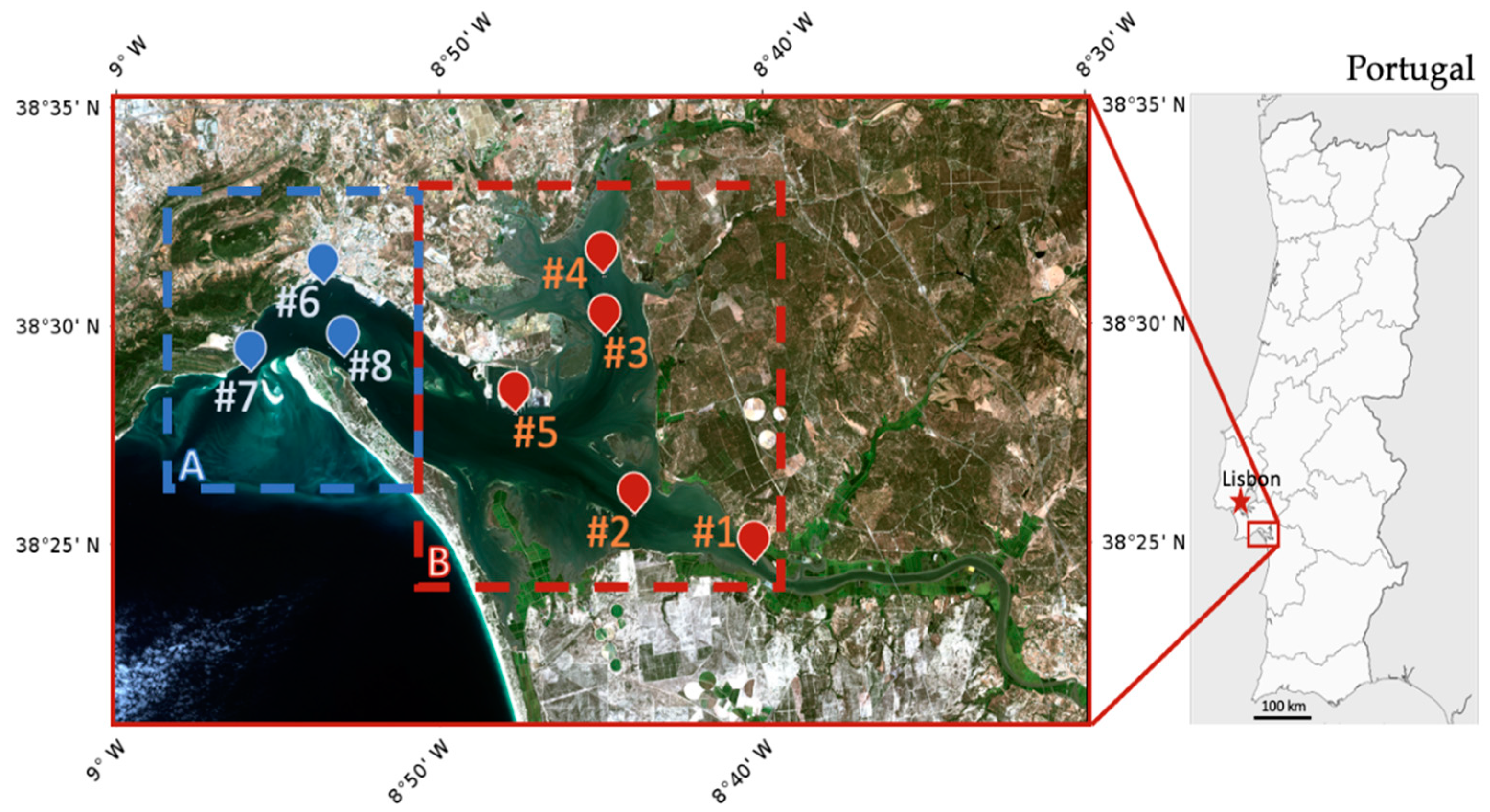
2.1. Study Area

The Sado estuary is a transitional system located near Setúbal, Portugal. It has a total area of 212.4 km2 [19], being, therefore, one of the biggest estuaries in Europe and the second largest national estuary (Figure 1). Given its high productivity, biodiversity and aesthetic value, it has been part of a natural reserve since 1980 [20]. Besides all the characteristics that make the Sado estuary a unique estuarine system, it is also a privileged place for aquaculture. The Sado oyster (Magallana angulata) is the main example of this activity in the region and is currently one of the main icons of the Setúbal region. In the context of WFD, nationally it is classified as a transitional water of typology A2- mesotidal well-mixed estuary [21].
The Sado estuary is characterized by a complex morphology and can be divided into two regions: (i) the outermost area (A in Figure 1), the Setubal bay, with 5 km wide, 20 km long and an average depth of 10m; and (ii) the innermost region (B in Figure 1), that presents a mixture of navigation channels and a vast intertidal zone of reduced depth (average depth of 10 m), relevantly influenced by the tide [22]. The connection to the ocean is made through a deep and narrow channel of approximately 1.5 km long and maximum depth of 50 m [23].
The Sado river flow can be considered low, varying on average from 0.7 m3/s in the summer to 60.0 m3/s in the winter [19,20]. Therefore, there is a strong influence of the tidal effect on the water circulation within the estuary [21,22]. The inflow and outflow of water is generally made along the two navigation channels (North and South channels, where stations 6 and 8 are located, respectively), according to the tide, with more intense currents in the South channel [24,25].
The estuary presents relatively low sun elevation during winter and higher wind intensities during spring-summer (hourly average with a maximum of ~8 m/s in 2018 and ~6m/s in 2019, Source: https://snirh.apambiente.pt (accessed on 26 November 2020)). These factors along with the tidal variation, the low water column depth and, consequently, the observed bottom resuspension, makes accurate ocean colour remote sensing challenging in this system.

2.2. In Situ Data

For the present analysis, 8 sampling stations distributed along the estuary, shown in Figure 1, were considered. The estuary was divided into two areas according to its morphologic characteristics and the variation of its physicochemical properties, as described earlier, thus stations #6, #7, and #8 were located in the outermost area (A) and stations #1 to #5 in the innermost region of the estuary (area B) (Figure 1). All sampling stations were located in optically deep waters (verified by the in situ measurements of Secchi depth). Monthly campaigns were performed between March 2018 and November 2019 within the framework of the AQUASado project. All campaigns were planned to start the water samples collection at similar tidal conditions (high water), to avoid the influence of the tide on the temporal variability of the WQ parameters, and to coincide with the S2-MSI satellite passage over the Sado estuary, when possible.
Surface water samples were collected and taken to the laboratory for quantification of aCDOM, Chl-a, SPM, and turbidity. It is relevant to note that the total number of samples for the different parameters may vary according to the quality control results and data availability.
Moreover, the absorption coefficients of phytoplankton (aphy) and non-algal particles (anap) were also obtained following the method described in [26]. These data were only used for the characterization of the study area and will be further analysed in a different work. Water temperature and salinity were also measured for site characterization purposes. The temperature was measured using an EXO2 Multiparameter Sonde (YSI) and the salinity through a high precision salinometer (Guildline Autosal 8400B) [27].

2.2.1. CDOM Absorption Coefficient

The methodology described in [26] was used to obtain the CDOM absorption coefficient (aCDOM (λ), m−1). Water samples were filtered in triplicate through a 0.2 µm pore size polycarbonate filter (Whatman). The absorbance readings of the filtrate were obtained at the range of 300–800 nm through a dual-beam spectrophotometer (Shimadzu 2600). From the average of the absorbance readings and the subtraction of the reference sample, the values obtained at each λ were multiplied by the light extinction coefficient (2.303) and divided by the cuvette length (0.01 m) [26].

2.2.2. Chlorophyll-a

Water samples were filtered using GF/F filters with 25 mm diameter and a pore of 0.7 μm (Whatman). The filters were then wrapped in aluminium and stored at −80 °C to be later analysed through high performance liquid chromatography (HPLC) (C18 column) to quantify the different phytoplankton pigments following the method described in [28] and adapted by [29]. For the extraction, 3 mL of a solution composed of 95% cold methanol, buffered with 2% of ammonium acetate and containing 0.35 mgL−1 of trans-β-Apo-8′-carotenal (as internal standard) were used. After placing the extraction solution in the sample test tube, the filter was grinded with a glass rod. Then, the tube was placed in the freezer (−20 °C) for 30 min after which it was placed in the ultrasound for 5 min. The test tube was then put back in the freezer (−20 °C) for another 30 min and, just after, centrifuged for 10–15 min at 4000 RPM (4 °C). Lastly, the sample was filtered and run in the HPLC machine.

2.2.3. Suspended Particulate Matter

SPM, defined as the dry mass of particles per unit volume of water sample (mg L−1), was determined following the standard gravimetric method described in [30]. A known volume of water sample was filtered through pre-ashed and pre-weighted Whatman GF/F filters (nominal pore size 0.7 µm and 47 mm diameter), with volume depending on the amount of material present in the water. At the end of filtration, the filters, including the outer edge of the filters, and filtration apparatus were rinsed with MilliQ water to remove any salt. The dry mass of particles collected on the filters was then measured with a precision balance.

2.2.4. Turbidity

The turbidity was determined with a portable infrared turbidimeter (Lovibond TB 210 IR) which quantifies the turbidity in nephelometric turbidity units (NTU) by measuring the light (λ = 860 nm) scattered at 90°, with an accuracy of ±2.5% of reading. The instrument calibration was checked before each sampling campaign using the calibration standards provided with the instrument (<0.1, 20, 200, and 800 NTU) and track the instrument stability. The turbidity was always recorded in triplicate for the same water sample and averaged.

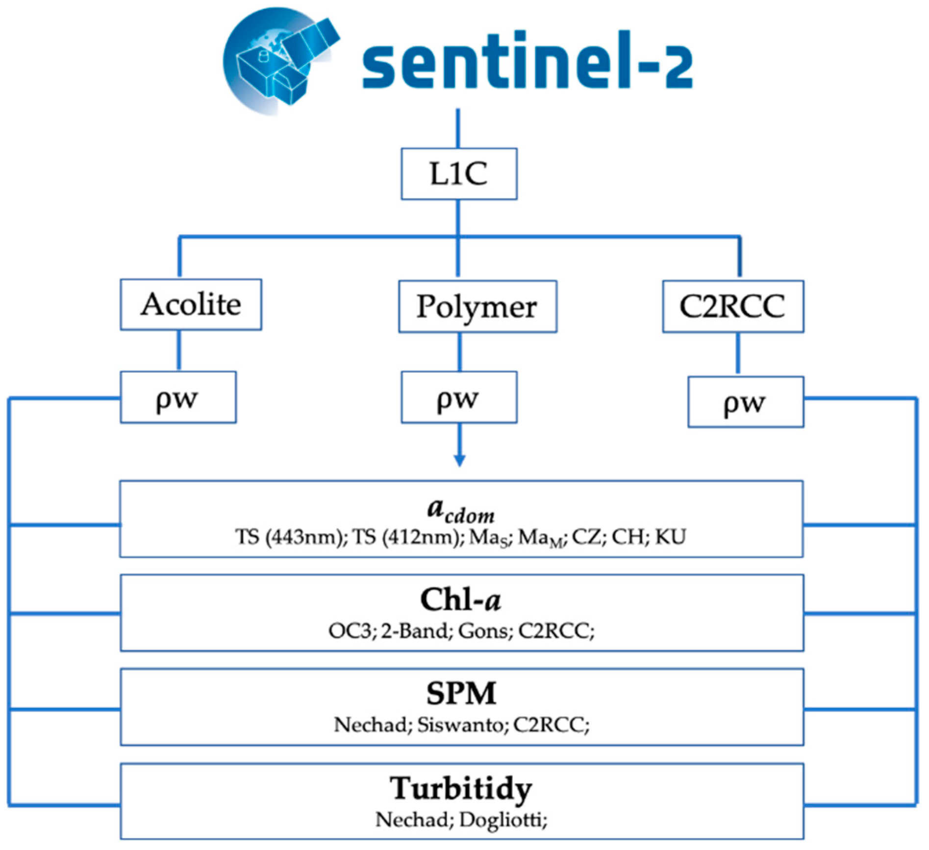
2.3. Sentinel-2 MSI Data

Sentinel-2 (A/B) MSI Level 1C images were used in the present study. The S2-MSI granules acquired between March 2018 and March 2020 were downloaded from Sentinel Scientific Data Hub (https://scihub.copernicus.eu/ (accessed on 26 November 2020)). Cloud free L1C images with coincident field campaign dates were used to compare satellite-derived data with in situ measurements or match-ups (processing chain shown in Figure 2). The images were re-sampled to 10 m as part of the pre-processing and the average of 3 × 3 pixels window centred on the sampling station was used for the in situ comparison and to perform the time-series.
To perform the matchups, the available images were filtered considering the time difference between the satellite passage and the in situ measurements. The time window chosen was ±2 h. The number of total match-ups depended on the AC processor used. To ensure high quality of satellite data, different quality flags were considered (Table 1). These quality flags are part of the L2 processing and, when raised, they indicate that something might have gone wrong during the data processing and that the retrieved product should be carefully analysed. Moreover, the IdePix (v2.2) was used on L1C images for pixel type identification.
Given the lack of in situ radiometric measurements for the direct test of AC, three AC processors were evaluated by testing a combination of AC + bio-optical algorithms (Figure 2). The AC processors tested were Acolite v20190326 (RBINS) [31], C2RCC v2.0 [32] and Polymer v4.12 [33]. The selection of the aforementioned AC algorithms was based on their free availability, and on the correcting effects that could be applied, such as sun glint and adjacency of land pixels, common sources of errors in transitional waters.
Acolite is an AC processor developed for coastal and inland waters. By default, it performs atmospheric correction using the dark spectrum fitting approach, but it can be configured to use an exponential extrapolation approach [34].
The C2RCC processor relies on a database of radiative transfer simulations of water-leaving reflectance and related top-Of-atmosphere radiances (satellite signal) [32]. The inversion of water signal and satellite signal is performed by neural networks and is fully described in [32].
Polymer AC is a coupled water-atmosphere model that uses a spectra-matching optimization approach to obtain a best-fitting combination of water and atmosphere unknowns, being one of its strengths to retrieve water reflectance in the presence of sun glint. This AC does not use exclusively the signal in the NIR, but it also uses all the available spectral bands in the visible [33].
It is important to note that these processors are all under active development but they are publicly available and are considered mature and useful to compare [35]. Each processor was used with its default settings, as this should be the best option for general use, without a priori knowledge of the water body or atmospheric conditions.
Once the image processing was complete, the atmospherically corrected outputs, i.e., water reflectance ρw or remote sensing reflectance Rrs (Rrs = ρw/π), were used to test different algorithms for WQ parameters retrieval (Table 2), with the aim of selecting the best processing chain for the study area. Several algorithms have been developed to retrieve WQ parameters from S2-MSI data. However, the majority of them are often calibrated regionally for the optical characteristics of the different sites. Thus, the performance of such algorithms outside their calibration region is a key topic. To address this matter, an algorithm intercomparison exercise was performed for the different parameters under evaluation. The selection of the bio-optical algorithms to test was conducted considering: (i) the similarity between the original ranges of the in situ parameters used for their calibration and the range of in situ parameters observed in this study; (ii) their good performance outside their calibration region based on the literature review; and (iii) their applicability to S2-MSI data.

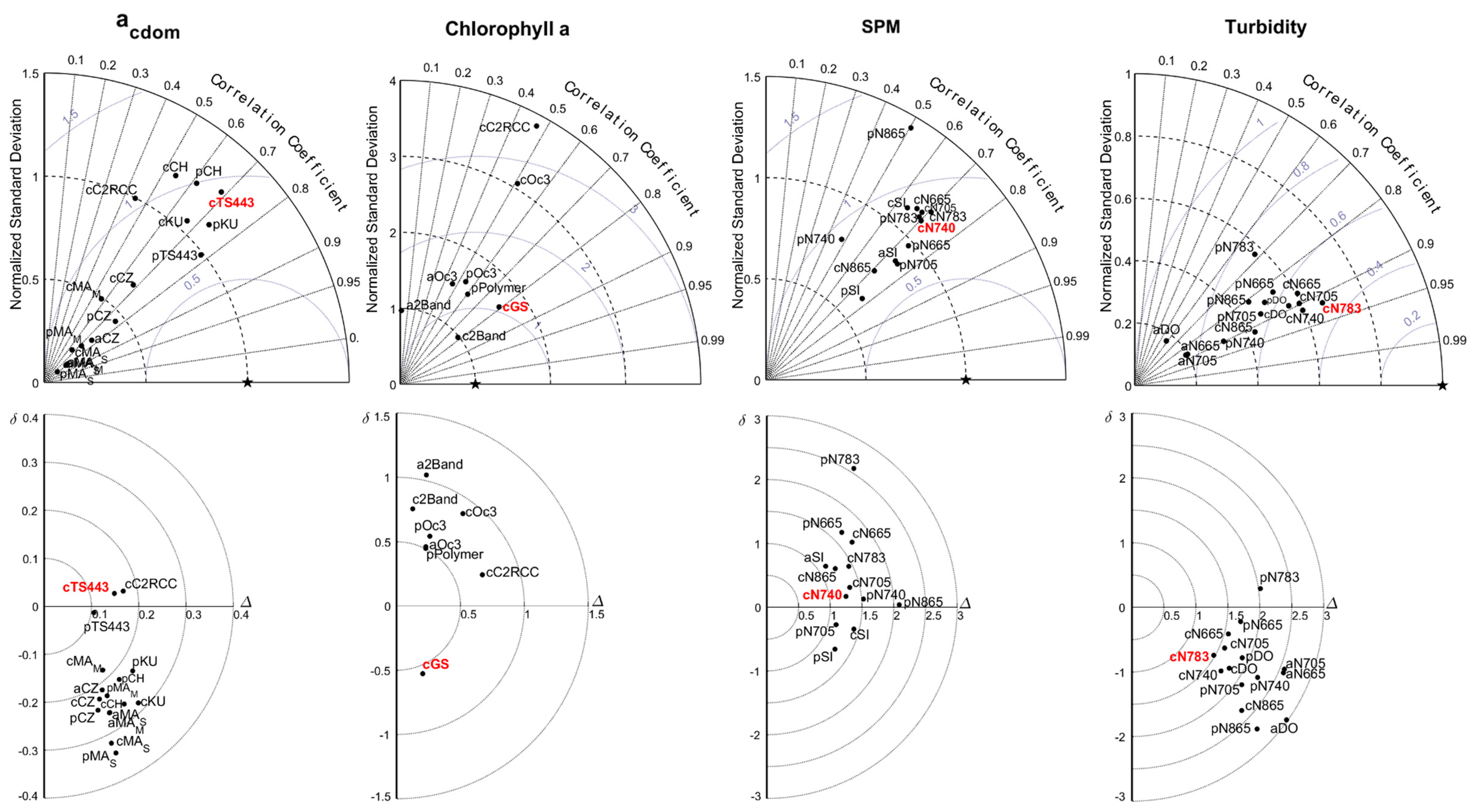
2.4. Statistical Indicators

To assess the agreement between the in situ observations and the satellite data, a statistical evaluation was performed using: linear regression parameters including coefficient of determination (R2), slope and intercept and uncertainty estimates including: root mean square deviation (RMSE), bias error (BIAS, δ), unbiased root mean squared error (URMSE, ∆), absolute percentage difference (APD), and relative percentage difference (RPD). The RMSE, the bias, and the APD were used to evaluate the accuracy of the match-ups and the RPD was used as an indicator of the systematic error (relative bias). These parameters can be defined as follows:
R M S E = i = 1 N   ( s a t i i n   s i t u i ) 2 N
B I A S = 1 N i = 1 N ( s a t i i n   s i t u i )
U R M S   = 1 N 1 = 1 N [ ( s a t i µ s a t ) ( i n   s i t u i µ i ) ] 2
A P D ( % ) = 1 N i = 1 N | s a t i i n   s i t u i | i n   s i t u i × 100
R P D ( % ) = 1 N i = 1 N s a t i i n   s i t u i i n   s i t u i × 100
where Sat is the satellite-derived data and in situ the observations collected in the estuary. N is the total number of samples, i is the sample index and µ s a t = 1 N i = 1 N s a t i – analogous definition applies for µin situ.
Statistical analyses of Chl-a are presented in logarithmic scale to account for the log-normal distribution of the bio-optical parameter [47]. According to [48] the RPD and APD were calculated without log-transforming the Chl-a values.
Additionally, summary diagrams such as Taylor and Target plots, referenced in [49] and [50], were used for a better visualization and inter-comparison of results. The Taylor diagram is based on the scoring of the normalized standard deviation (STDsat/STDin situ, [51]) and correlation coefficient (R). The Target diagram summarizes the scoring of the URMS and BIAS instead.

2.5. Time-Series Analysis

The statistical indicators described in Section 2.4 were used to select the best processing chain from the match-ups intercomparison exercise and perform a spatio-temporal analysis of the different WQ parameters, with the main objective of evaluating the capabilities of S2-MSI imagery for continuous monitoring of WQ variability in estuarine systems.
The best performing combination of AC + bio-optical algorithms was applied to all cloud-free L1C images sensed between March 2018 and March 2020. As done for the match-ups exercise, quality flags were considered to ensure the highest quality of satellite data.
Given the strong variability of the in situ data and the high dynamic that characterizes the Sado estuary, the time-series analysis was performed separately for the region A (outermost area) and the region B (innermost area) (Figure 1). The time-series performed with RS products and in situ observations considered the average of the pixels corresponding to the sampling stations included in each of the areas. Moreover, the seasonal variability (astronomical seasons) of the WQ parameters in the whole estuary and its adjacent area, is provided through high resolution maps.

3. Results

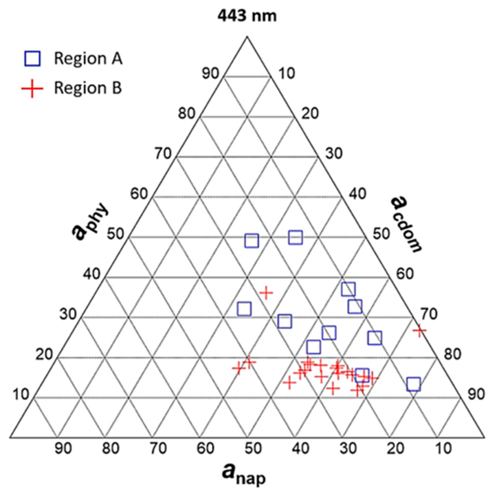
3.1. Study Area Characterization

Based on the monthly surface data collected in situ between March 2018 and February 2019 analysed in the present study (see Section 2.2), the estuary presents clear seasonal patterns of the physical and chemical properties (Table 3) with a clear tendency to find higher values of aCDOM, Chl-a, SPM, and turbidity during spring and summer. Furthermore, the estuary should not be considered spatially homogeneous. The innermost region of the estuary (B) shows higher values of the optically active components and a greater susceptibility to seasonal variations of the weather, given the greater thermal amplitude observed.
The Sado estuary is optically dominated by CDOM, as observed in Figure 3, with higher values of aCDOM compared in respect to phytoplankton and non-algal particle absorption coefficients, aphy and anap respectively. Figure 2 shows the dominance of aCDOM mainly in stations located in area B, showing smaller contributions of anap and aphy. It should be reminded that anap and aphy are only here presented to characterise the study area and will not be further analyzed in the present study. In region A, the contribution of aphy was slightly higher. However, aCDOM remains dominant in most of the stations located in this area. The important contribution of the aCDOM (443 nm) even in stations located in area A, allows to classify the whole estuary as optically complex with Case 2 waters [52], regardless of the studied period and the tidal conditions.

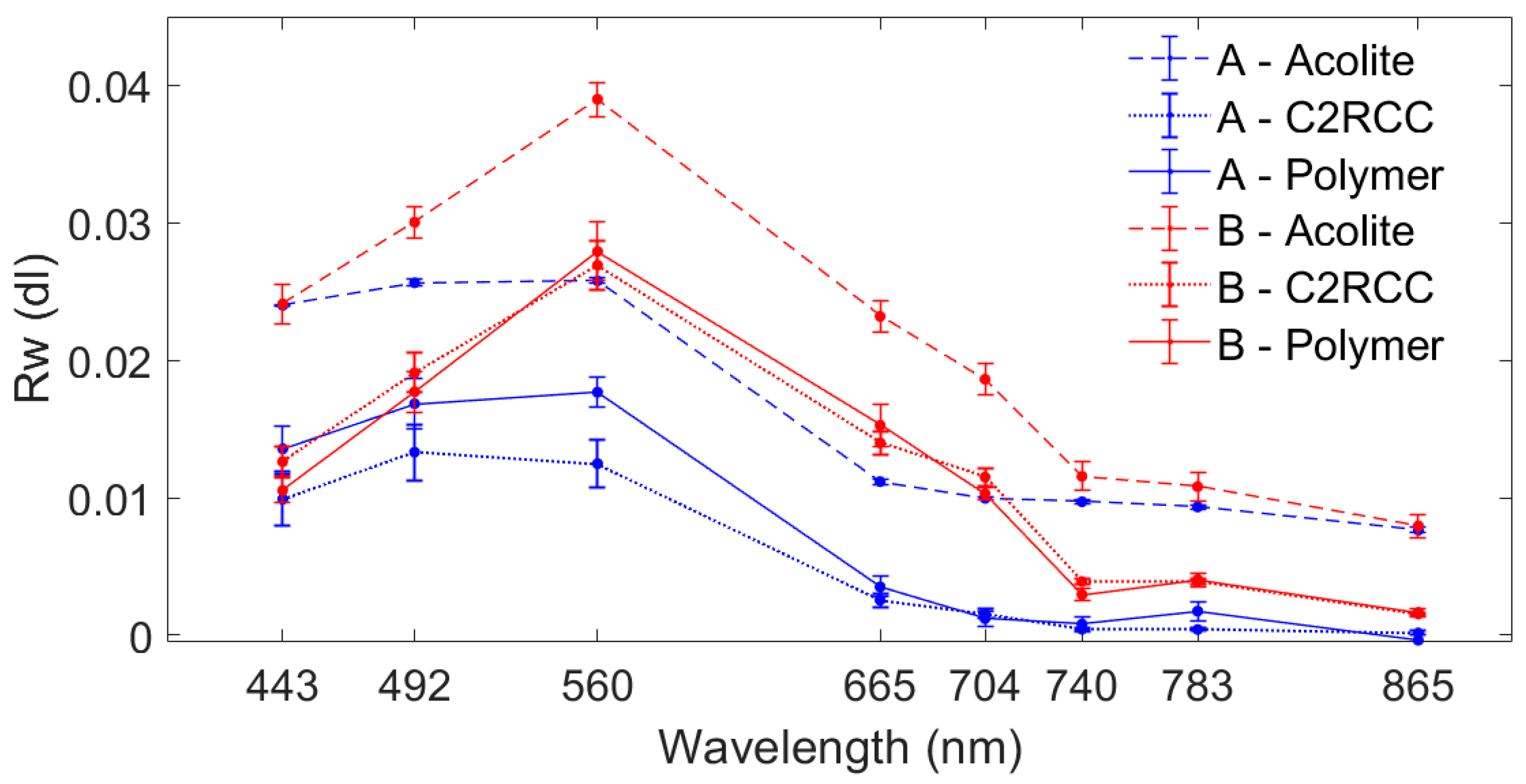
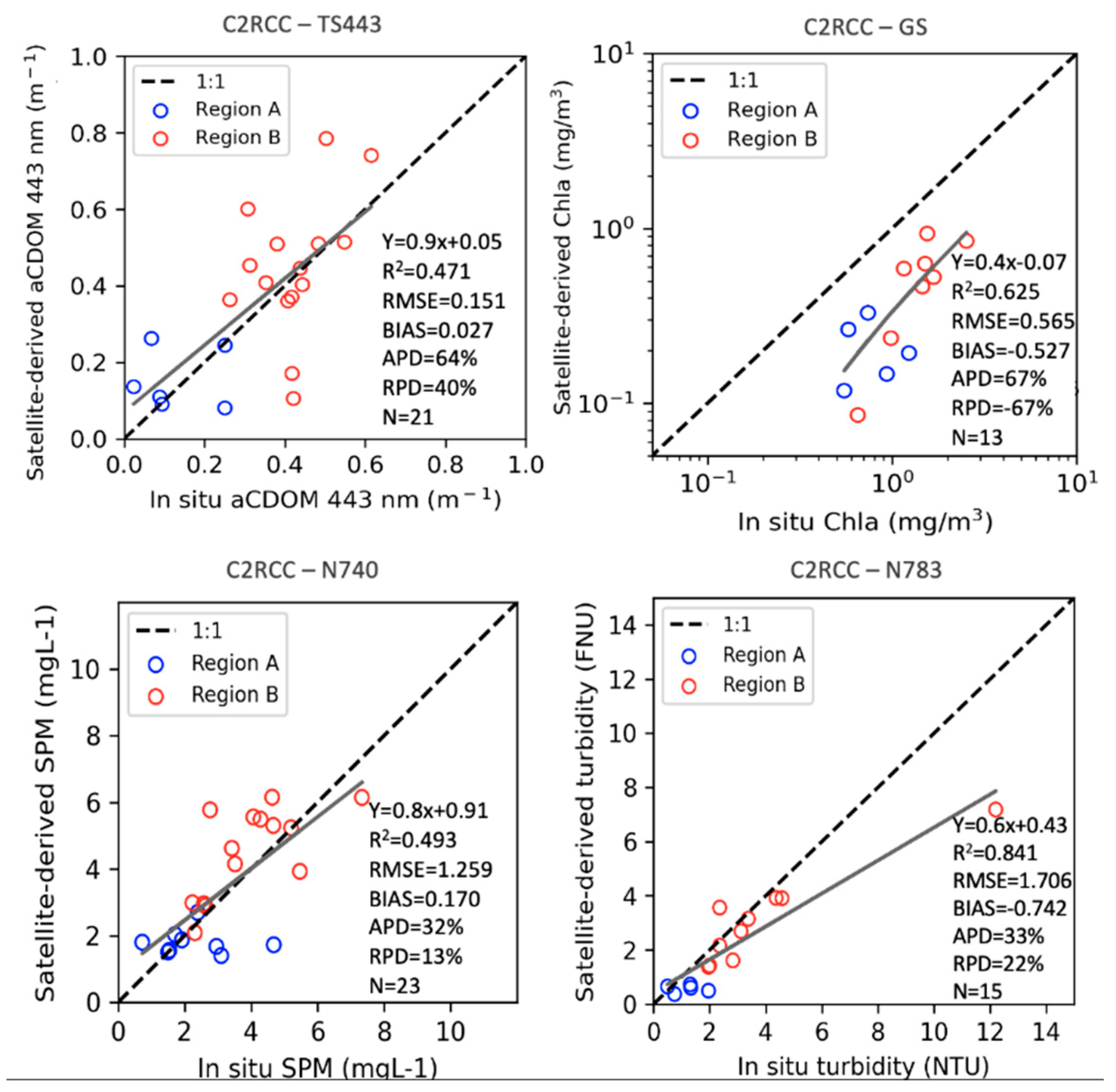
3.2. S2-MSI Match-Ups

For this study, the combination of AC and bio-optical algorithms were evaluated against in situ values of the different WQ parameters. An algorithm intercomparison exercise was performed for the available match-ups with the objective of selecting the best processing chain for a spatio-temporal analysis of the different WQ parameters under investigation. Taylor and Target diagrams were used for the selection of the best performing processing chain.
Even if no in situ radiometric measurements were available for a thorough comparison, the ρ w spectra derived from the matchups of the three AC processors were compared separating the two regions of the estuary (Figure 4).
Figure 4 shows that Acolite retrievals are significantly higher across the whole spectrum compared to the other ACs. In spite of this, similar shapes were obtained by the three processors. From a visual inspection, it can be noted a difference between the spectral shapes of areas A and B. In particular, for area B, ρ w in the blue, is lower compared to the green region of the spectra, i.e., the green peak is more pronounced than in area A. This could be partially due to higher importance of CDOM (aCDOM) and sediments (anap), which agrees with in situ measurements (Figure 3). Moreover, it can be observed that reflectance in the NIR region of the spectra is higher in area B compared to A, which matches the higher SPM found in the inner part of the estuary.
Regarding aCDOM, AC-C2RCC and Polymer showed the best performance (mean APD = 79% and APD = 68%, respectively) when combined with the bio-optical algorithms, compared to the results obtained using Acolite (mean APD = 164%). In the Taylor diagram (Figure 5), the TS443 and KU algorithms combined with Polymer (pTS443 and pKU) were closer to the reference (represented by a star). Considering the AC-C2RCC processor, the KU, CZ, and TS443 were the best combination performing algorithms. In the Target plot, the TS443 algorithm showed the results closest to the reference (zero), both combined with Polymer and AC-C2RCC. All other processing chains (except AC-C2RCC) underestimated the aCDOM. Among the algorithms that showed the best performance, the TS443 was the one with the slope values closest to 1 (0.9 with AC-C2RCC and 0.8 with Polymer), and the lowest RMSE (0.151 and 0.106, respectively for AC-C2RCC and Polymer) compared to the other algorithms (Table 4).
For Chl-a, combining the results obtained with the Taylor diagram and the target plot, the bio-optical algorithm/AC processor combination that compared best with the in situ data was GS with AC-C2RCC (cGS) reflectances. For this processing chain, the highest determination coefficient (R2 = 0.63) was obtained, while the remaining statistical parameters (RMSE, bias, APD and RPD) were the closest to zero (Figure 6). It should be noted that the application of 2-Band algorithm [41] to AC-C2RCC images also produced good results (the second best), superior to the ones of the standard Chla-C2RCC algorithm and even of OC3 (Taylor plot, Figure 5). On the other hand, the standard algorithm from Polymer (pPolymer) showed better results than the standard algorithm from C2RCC, but the first processor failed in the quantification of Chl-a using GS and 2-Band algorithms. In general, the satellite-derived data tended to overestimate the in situ data (except the combination with the GS algorithm). The retrieval of Chl-a remains relatively inconsistent, with large differences between satellite and in situ observations (high APD values).
For the SPM and turbidity products, better results were obtained when NIR bands were used. Considering the rather low measured SPM and turbidity values, signal in the NIR was expected to be low and a better correlation with the red bands could be expected. From the S2 extracted spectra (Figure 4) this is clear for region A, but less evident in region B. However, a poor relationship was found using the red bands for region A (not shown), which could be partially due to the overlap of this band with the location of the Chl-a absorption peak which might be affecting the retrieval of SPM and turbidity at this wavelength. Considering this and given the low number of match-ups available for region A, the dataset was not separated by region and thus, the general performance of the algorithm was used to select the best performing AC+algorithm. It should be noted though that for the clearer waters in region A the correlation is low (blue signs in Figure 6), thus results using the NIR bands should be considered with caution for this area.
For the SPM product, the best results were obtained from Polymer in combination with Nechad algorithm [44] at 705 nm (pN705) (R2 = 0.57, APD = 26%). However, this algorithm decreased its performance when applied to images processed with the AC-C2RCC. On the other hand, with AC-C2RCC, good results were also obtained, using Nechad algorithm for 740 nm (cN740) (R2 = 0.49, APD=31%) (Figure 6). Interestingly, the same algorithm (for the same wavelength) showed a worse performance when applied to images processed with Polymer (Table 4). For SPM, Acolite + bio-optical algorithms were the combinations that presented the worst performance (APD always > 150% except from aS, where APD = 31%) and the only ones in which there was a tendency to overestimate in situ values, suggesting that ρ w   is overestimated compared to other AC (Figure 4). From the set of results, it was the application of Nechad for the 665 and 705 nm wavelengths that showed a greater consistency in the results between the different processors, although they did not have the overall best performance when compared with the in situ dataset.
The highest agreement between the satellite and the in situ turbidity data was achieved by applying Nechad at the wavelength of 783 nm to the images processed with AC-C2RCC (cN783, R2 = 0.84, APD = 33%) (Figure 6). Overall, this AC processor presented good results for the set of algorithms and bands tested. Additionally, AC-C2RCC showed a tendency to underestimate satellite-derived turbidity data in comparison to the in situ measurements (negative RPD for all the algorithms). The application of the Dogliotti algorithm [46] generated results similar to those of Nechad for AC-C2RCC images, as expected. With Acolite, the application of Nechad to bands 740, 783 and 865 nm showed a relevant decrease in the quality of the match-ups results, when compared with the lower wavelengths.
Overall, two out of the three tested AC processors algorithms, AC-C2RCC and Polymer plus bio-optical, seemed to provide results more comparable with in situ data for the selected study area (Table 4). The combinations (AC+bio-optical algorithms) tested with these two processors presented similar results for all the parameters and can be considered more suitable for the study area than the combinations using Acolite (mean APD = 254%), which showed a general overestimation of the in situ values (mean BiasACOLITE = 2.78; mean BiasC2RCC = 0.04; mean BiasPOLYMER = −0.07). Even though Polymer combinations have outperformed AC-C2RCC combinations in specific cases, such as in the quantification of CDOM or SPM, it did not present satisfactory results for Chl-a. Considering that AC-C2RCC combinations showed good capabilities for all these parameters, the best performing AC-C2RCC processor plus bio-optical algorithms were selected for the time-series analysis for being the best combination for the set of parameters analysed. In accordance, only the best match-ups results of the application of the algorithms to AC-C2RCC images will be presented in this section (Figure 6). The full dataset of statistical results is available in Table 4.
Since the combinations using the AC-C2RCC were chosen as overall best performing, the algorithms selected to perform the time-series analysis were the following: cT443 (aCDOM), cGS (Chl-a), cN740 (SPM), and cN783 (turbidity). The table contemplates the data of the average of 3 × 3 pixels centred in the pixel of the sampling stations. The best performing processing chain of eaxh parameter are highlighted in bold.
Overall, for the set of parameters tested, encouraging results were obtained in the satellite data intercomparisons process, which indicates the usefulness of MSI images to monitor water quality parameters in the Sado estuary.

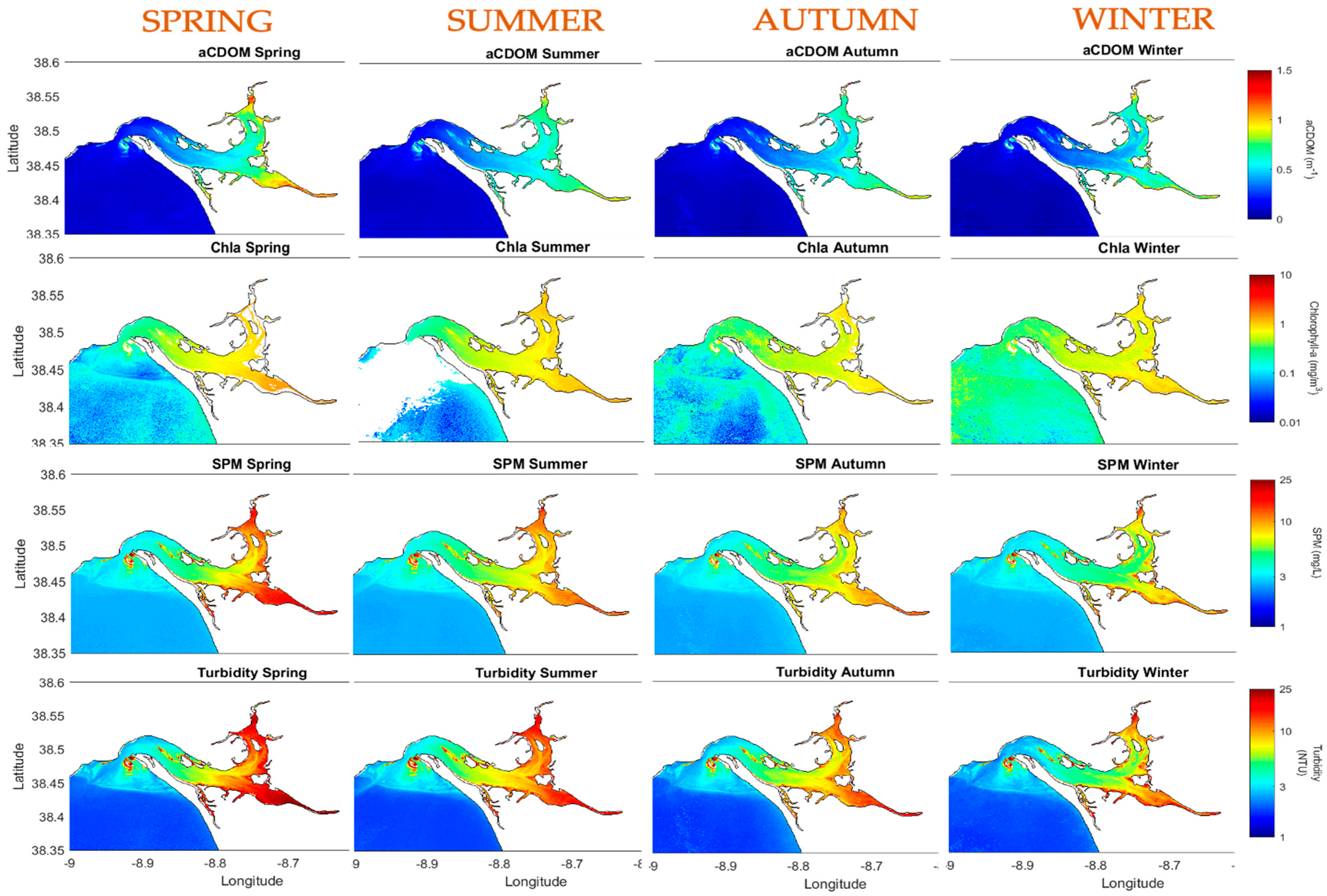
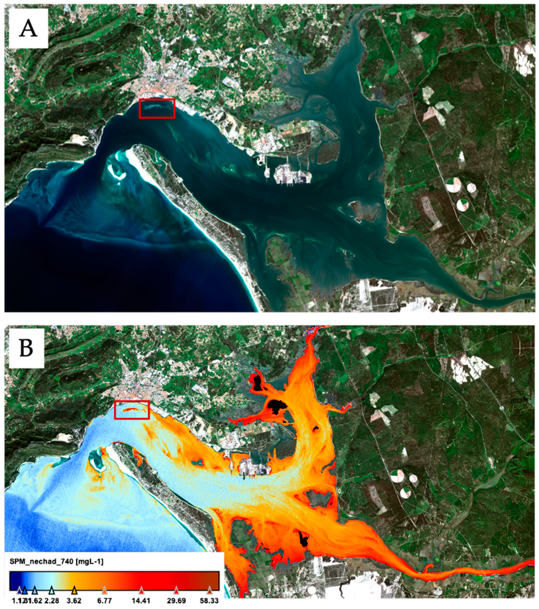
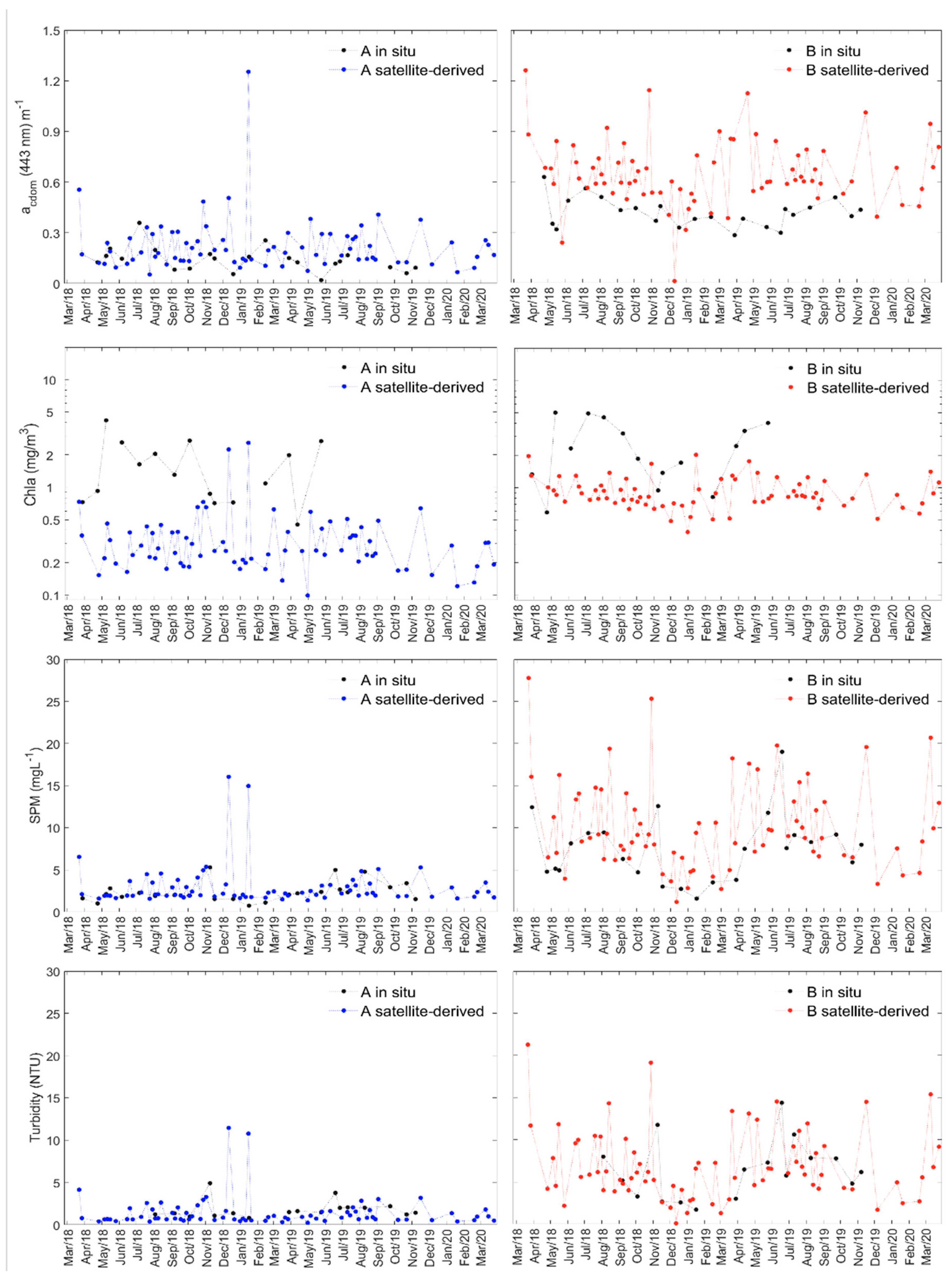
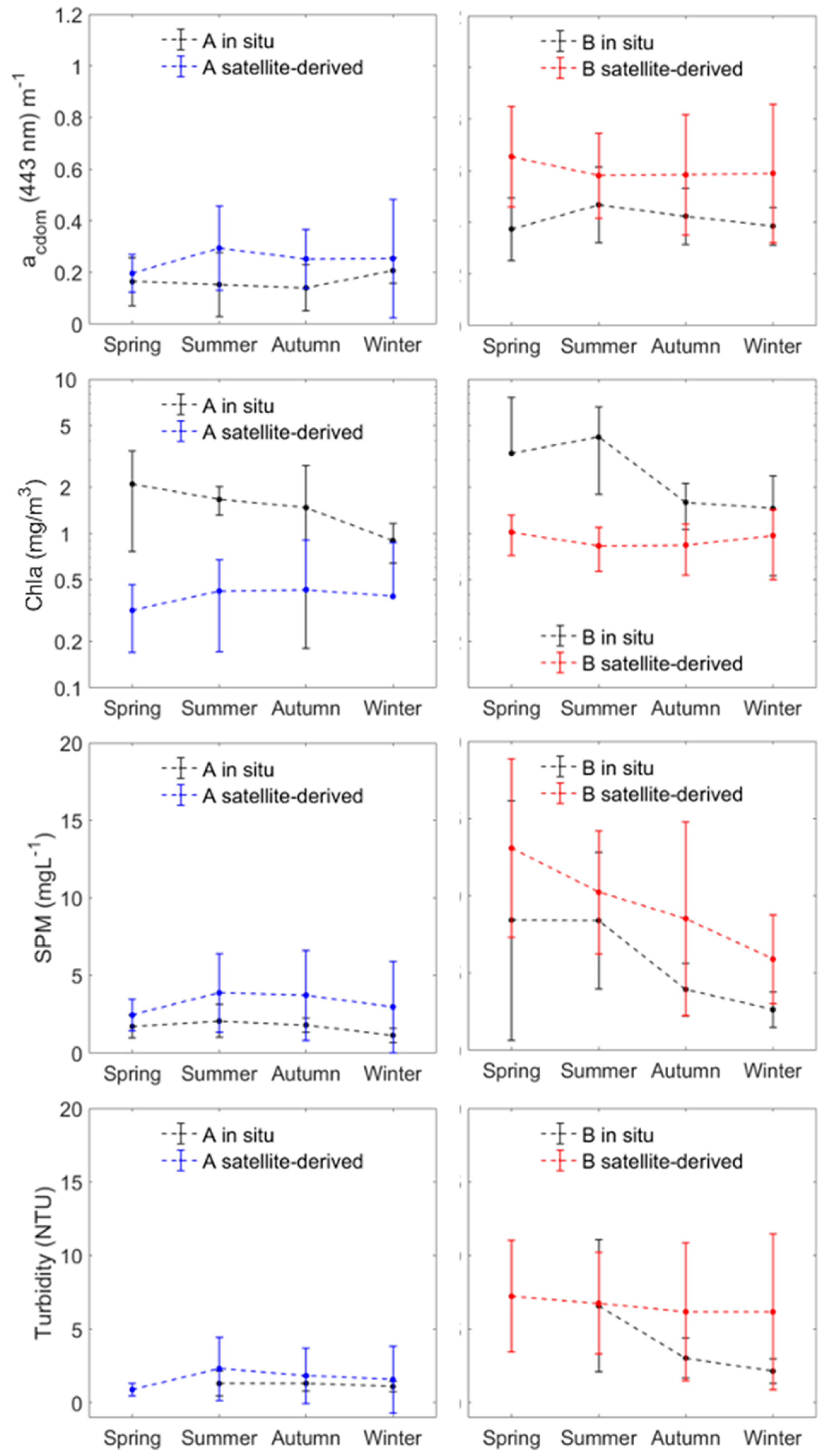
3.3. Spatio-Temporal Analysis: Sado Estuary Case Study

To demonstrate and evaluate the usefulness of a consistent Sentinel-2-derived WQ data record, we present here a spatio-temporal analysis of the four WQ parameters under investigation for the Sado estuary. To do so, the best performing processing schemes chosen during the intercomparison part of the present study were selected and applied to S2-MSI time-series, i.e., AC-C2RCC-TS443 for aCDOM, AC-C2RCC-GS for Chl-a, AC-C2RCC-N740 for SPM, and AC-C2RCC-N783 for turbidity (Figure 6). Moreover, the time-series analysis was performed separately for the two different regions of the estuary, given the high optical variability that characterizes this transitional system.
Figure 7 and Figure 8 show the time-series of the different parameters considering the spatially averaged observations. From a visual inspection, it is hard to observe a clear seasonal variability of any of the selected parameters in area A. Moreover, region B presents a greater amplitude (over a short time, due to tidal variability) of values in respect to region A, which remains relatively constant. This might lead to bigger uncertainties associated with satellite-derived products over region B due to higher optical variability and greater interaction between the optically active compounds. Therefore, a worse performance of the bio-optical algorithms is expected. Moreover, the greater amplitude of values will lead to difficulties in detecting WQ anomalies without a consistent climatological record of the area of interest. On the other hand, S2-MSI time-series may allow us to better understand the short-term variability which would be highly laborious through in situ observation.
For a better visualization of the seasonal patterns, high spatial resolution seasonal maps of the full estuarine system are provided in Figure 9. For all the set of parameters, the highest values were found in Spring and Summer, mainly in the inner region of the estuary, following the tendency shown by the field measurements.
Regarding the aCDOM (443 nm), the seasonal maps show higher values during Spring within the whole estuary. However, the seasonal average of in situ aCDOM (Table 3) shows that the highest values were obtained in Summer in the innermost region of estuary, and in winter in region A. In this region, the outermost area, the greatest differences between the seasonal averages of satellite-data and in situ (Table 1) were found in summer (0.14 m−1) and in autumn (0.11 m−1), while spring and winter presented the smallest variations (0.03 and 0.05 m−1 respectively). In region B, the greatest differences were in spring (0.28 m−1) and in winter (0.20 m−1), while the smallest in summer (0.11 m−1) and during autumn (0.16 m−1). Even if the satellite seems to be able to follow the in situ trend in both areas, the satellite-derived values slightly overestimate the field observations most of the time. This can be clearly seen in the time-series plot, especially in region B between April and October 2019.
For chlorophyll-a, it was possible to observe a significant difference (mean APD = 391%) in terms of absolute values between the in situ data and the satellite-derived ones (Figure 7). This deviation between datasets seemed to be more evident during Spring and Summer, both in region A and region B. It is possible to observe that the satellite-derived data were not able to match the highest chlorophyll in situ values found during the sampling period, presenting a significant underestimation in comparison to the in situ observations. During Autumn and Winter, when field Chl-a measurements were lower, a greater similarity between the datasets was found. In general, region B presented slightly higher Chl-a values than region A, as would be expected, given the in situ variability observed. As such, the MSI sensor was sensitive to the spatial variability of the chlorophyll-a in the Sado estuary. This spatial variability of Chl-a becomes more evident when looking at the entire estuary and its surrounding region (Figure 9). It should be noted that in Summer, it was not possible to obtain valid values for the region in the coastal ocean (Figure 9) due to sun glint occurrences that led to an overcorrection in the atmospheric correction part of the processing, which, combined with low concentrations of chlorophyll, resulted in invalid Chl-a values. During winter, it was also possible to observe high chlorophyll values in the interior of the estuary and in the region of the coastal ocean (higher values than during spring).
Regarding SPM, Figure 7 and Figure 8 show that the derived product can clearly capture the temporal variability and potential anomalies in water conditions. As expected, higher values were observed in the inner region of the estuary at all seasons, being spring and summer the seasons with the highest levels of suspended solids within the estuary. As well as for aCDOM and turbidity, the SPM retrieved recurring to the S2-MSI presented a slight overestimation of the in situ observations.
As already mentioned in the match-ups section, the turbidity product was the best represented WQ parameter using S2-MSI data. This can be easily observed also from the time-series plots, where the satellite-derived turbidity followed the in situ observations with high similarity, showing the great potential of this satellite for routine monitoring of this important parameter. Again, the highest turbidity levels were reached in spring and summer, with higher concentrations in the inner region of the estuary. It is important to note that despite the match-ups stations being optically deep at the time of the sampling, for the time-series it was not possible to know it in advance. Moreover, in this study, it was not possible to assess if the shallower regions of the estuary were influenced by the bottom signal therefore Figure 9 should be interpreted with caution.

4. Discussion

4.1. Algorithms Intercomparison Exercise

The principal objective of this study was to evaluate the potential use of high spatial resolution satellite data to estimate water quality (WQ) parameters in a highly dynamic system. For this purpose, different processing chains (AC plus WQ algorithms) have been selected and applied to S2-MSI imagery in order to evaluate the usefulness of this satellite for water quality monitoring in the Sado estuary.
According to the results, the statistics indicate consistency between the satellite-derived values and in situ observations of turbidity, indicating that this parameter is the best WQ parameter to be retrieved via S2-MSI data. However, the agreement is also relatively strong for SPM and aCDOM for the study area, while the Chl-a product showed some limitations and higher errors associated (Table 4).
Even if no field radiometric measurements were available to directly assess the performance of the AC processors, AC-C2RCC and Polymer combined with bio-optical algorithms were the combinations that provided the most comparable results to the in situ data. Similar results have also been discussed by Warren et al. [35], where different AC processors have been tested on S2-MSI data showing that AC-C2RCC and Polymer outperformed Acolite for applications in coastal waters. Pereira-Sandoval et al. [53] also showed similar results, pointing out the good performance of these two ACs in Spanish inland waters and suggesting the application of a water type classification to improve the performance of the processors.
Polymer and AC-C2RCC were the processor that presented the smallest reflectance values between the processors tested in this study. An underestimation from the Polymer processor was observed in other studies. Steinmetz et al. in [33,54], the authors pointed towards a miss-estimation of the wind speed from the afore-mentioned processor that might lead to an over-correction of the model, resulting in a significant reduction of the total signal, which could explain the invalid Chl-a values obtained using this processor. Again, the lack of in situ radiometric measurements did not permit to deeply explore the performance of the ACs in this study area. Even if the Polymer processor, in combination with bio-optical algorithms, outperformed AC-C2RCC in some cases, the neural network methodology was selected as it provided the best overall combinations performance and was used to perform the time-series analysis.
In complex waters, the CDOM generally increases absorption (reducing reflectance) in the blue bands while the SPM causes an increase in reflectance in the green and red bands due to scattering [53,55]. In the present study, region B of the estuary presented greater contribution of SPM and turbidity and, in fact, the water-leaving reflectance of all AC processors was relatively higher in the green-red bands compared to region A (Figure 4). However, very similar values were observed between the two areas of the estuary in the blue region of the spectra, where also higher values were expected. In conditions of high SPM concentration, the aCDOM algorithms that use the blue/green-red band ratios tend to underestimate the measured aCDOM. These factors may have affected the performance of regionally calibrated algorithms (i.e., MAS, MAM, CZ, CH, and KU) that, in general, underestimate the aCDOM retrieval in conditions of higher SPM concentrations. In cases where the aCDOM does not co-vary with Chl-a, as in the present study, this can significantly affect the bands in the blue to green part of the spectrum due the overlap on the reflected signal [56,57,58,59]. Thus, it is necessary to know the variation of the optically active components present in the water to find alternatives that provide greater accuracy to the retrieval of WQ parameters by satellite remote sensing.
Regarding chlorophyll-a, in the study conducted by Pahlevan et al. [9], the 2-band algorithm originated negative retrievals for low concentrations of Chl-a. The authors considered that this was somehow expected as 2-band algorithms are usually designed to be applied in highly eutrophic waters, a category in which the Sado estuary does not fit. Pereira-Sandoval et al. [53] tested several AC processors to S2-MSI data and observed that, for inland waters with low concentrations of chlorophyll-a, Polymer showed slightly worse results in the NIR bands than C2RCC. Possibly, the existence of low Chl-a values in the Sado estuary, combined with a possible overcorrection performed by Polymer processor, could be the cause of the absence of valid Chl-a values when the GS and 2-band were applied to the data derived from this processor. Interestingly, Chl-a processed by Plymouth Marine Laboratory (PML) using the Calimnos processing chain [60] also did not produce Chl-a matchups with our in situ data for the Gons algorithm [42] coupled with Polymer AC, demonstrating consistency with our results (data not shown). Thus, deriving reliable Chl-a data from S2 is still challenging and further developments are needed. In this context, the on-going H2020 CERTO project (www.certo-project.org (accessed on 26 November 2020)) is likely to provide relevant outputs. This project aims to produce improved satellite data that should be harmonized across different types of complex waters, i.e., from lakes to the sea, with a particular emphasis in transitional waters. Considering its great potential, future work will include testing CERTO’s products, which will be delivered during the project.
Regarding SPM and turbidity retrieval, given the strong relationship between the two parameters (R2 = 0.92 in our study area) their relation is worth to be mentioned. Clear differences can be noticed between the turbidity and SPM S2-MSI retrieval, with turbidity presenting overall better correlations with in situ data. This might be caused by different factors. Firstly, turbidity parameter is less subject to in situ measurements errors than SPM. Röttgers et al. [61] demonstrated that significant uncertainties can be associated with most of the SPM measurements. Their results showed that these errors were mainly associated with salt retention and loss of filter material during washing and drying procedures. Moreover, turbidity is an optical parameter highly related to backscattering [45] and thus to reflectance. To explain the poorer retrieval of SPM using a global algorithm with respect to turbidity, the differences between the SPM and turbidity retrieval algorithms should be considered as suggested by [45]. In fact, since turbidity (a measure of side-scattering) is an inherent optical property (IOP), it is not necessary to consider the potential variability of mass specific optical properties, while SPM algorithms do. On the other hand, SPM retrieval algorithms will also be sensitive to particle size, density, and refractive index, which can be important sources of regional variability for retrieval of SPM concentration.
Furthermore, in Figure 6 it is possible to see that the selected algorithms for SPM and turbidity (which use NIR bands) perform better in region B (more turbid waters) compared to region A (clearer waters). Considering the strong spatial gradients, the non-linearity of SPM optics properties in estuarine environment [62] and the interaction with different optically active constituents such as phytoplankton cells, it is key to develop algorithms that are calibrated regionally to accurately quantify SPM from satellite data. Future work will include further investigation on the performance of single-band algorithms considering the different optical properties that characterize the different regions of the estuary. The work will focus on the development of a switching band algorithm that takes into account the different optical properties of region A and region B.
In general, the results of the present study suggest that for satellite-derived aCDOM, Chl-a and SPM, regional approaches should be adopted for Portuguese transitional waters. Regarding turbidity, the statistical results are encouraging, with reasonably accurate turbidity retrieval using a global algorithm, at least for Region B. As a whole, for the Sado estuary, there is still the need for a more robust database accompanied by in situ and orbital radiometric measurements from remote sensors.

4.2. Spatio-Temporal Analysis

All the analysed parameters showed strong spatial variability within the estuary, as expected. This indicates that to analyze these parameters using in situ measurements, multiple sampling points are needed to fully represent the study area, which is not always feasible. In turn, the seasonal variability of the WQ parameters seemed to be well captured from the S2-MSI satellite products, evidenced in the time series by overlapping the in situ with the satellite-derived data.
For all parameters, higher values were obtained in the interior area of the estuary and during Spring and Summer, in concordance with previous studies [18,63], mainly due to phytoplankton blooms and bottom resuspension caused by stronger wind regimes in the referred period of the year. In the period here studied, the highest SPM values were also found in spring and summer, even if precipitation is stronger in autumn and winter, when higher terrigenous inputs from the rivers are expected. The higher values of SPM (which are historically found in spring) are related to the phytoplankton spring blooms and bottom resuspension due to stronger wind regimes, and not to terrigenous inputs of the SPM [64].The aCDOM (443) parameter did not correlate or co-vary with the Chl-a, but it had an inverse relationship of R2 = −0.57 (p < 0.05) with salinity (not shown here). This suggests that most of the CDOM’s origin is not local (e.g., from the phytoplankton derived components), but rather from bottom resuspension processes due to stronger wind regime within the estuary during spring/summer and from increased rain and riverine input mainly during winter [64,65].
As already mentioned, Chl-a was the parameter that presented the greatest challenges in achieving accurate satellite-derived data. However, it was possible to obtain useful results on the patterns of temporal and spatial variability of the phytoplankton proxy using Sentinel−2 MSI in the Sado estuary. The highest concentrations were found in spring and summer, as expected, even if high values of Chl-a were also observed during winter in the inner region of the estuary. It is also interesting to note that the region of the coastal ocean presented unexpected variation patterns, showing higher values of Chl-a during winter with respect to spring. Furthermore, during summer, the same region did not present any valid Chl-a data, suggesting that the selected algorithms may not be suitable for Chl-a retrieval for the clearer waters in the coastal ocean which present different optical properties, more similar to the open ocean.
Overall, the time-series analysis of all the studied parameters was found to be in agreement with the historical climatological data available for the area and, therefore, the use of the S2-MSI sensor can be considered useful for water quality analysis over the Sado estuary using the selected best-performing processing chain. The high spatial resolution maps provided for the study area are a relevant achievement since no such information was available until the present work, although improvements regarding the bottom effect should be pursued in future work.

4.3. Applicability of Satellite RS Products to WFD

The EU WFD requires that all Member States achieve and/or maintain good ecological status of their water bodies, including estuaries. Under the directive, the assessment of WQ is based on the deviation from a predefined reference condition. However, as discussed by [66], this is one of the most complex, and still under discussion, points of its implementation. For the Sado estuary, in fact, the phytoplankton Chl-a is one of the few water parameters that have a well-defined classification system to assess the ecological status of the water body. According to the range of values observed during the period under analysis, the concentrations never exceeded the reference value for the highest salinity class (6.67 mg m−3 for salinities higher than 25 [67,68]) being the observed Chl-a concentration (both in situ and satellite-derived) always <5 mg m−3, and therefore indicating that the Sado estuary has currently no clear sign of eutrophication problems. However, it should be reminded that the in situ data considered was always collected at high tide conditions. Higher values might be encountered during low tides.
The lack of historical data for the other physicochemical parameters in the Sado estuary increased the level of difficulty in applying RS WQ products in the context of ecological quality assessment, under the WFD. The definition of reference values is crucial to further explore the potential of RS in the context of the WFD, for which S2-MSI satellites have a great potential. The provided time-series of the WQ parameters obtained through remote sensing observations are crucial to define baseline levels and allowed to confirm the values used to assess the normal variation patterns (i.e., SPM < 20 mgL−1, data not shown). This will help decision-makers to detect potential anomalies and support further studies on ecological aspects. Moreover, these high-resolution maps provide key information to implement effective and meaningful monitoring programs for WQ assessments under the WFD.
Considering the great importance of CDOM as a WQ indicator, we consider that more efforts should be put to retrieve more accurate CDOM absorption values from the S2-MSI data. As discussed previously, aCDOM is strongly related to salinity [69] and therefore could be used by policymakers as an indicator of fresh-water input within the estuary or to infer drought periods.
One major benefit of using remote sensing data to support the monitoring of surface water status is the capability of providing systematic observations of the whole water-system. The high revisit frequency (5 days) allows an easier detection of small-scale changes and a more synoptic view of the water body. However, a relevant drawback of optical remote sensing data is that cloud coverage and sun glint effects may seriously affect its usefulness [70]. In the present work, only an average of 55% of the total images available (over the 2 years period under investigation) were cloud-free and focused on periods with good atmospheric conditions. This means that image availability is non-homogeneous around the year and can make routine monitoring challenging.
As an example of the applicability of S2-MSI images for water quality assessment, Figure 10A shows the RGB image acquired on 19 February 2020 by the satellite S2A, that captured the dredging activities conducted in the Sado estuary. In the RGB image (top), the sediment plume produced by the dredge is clearly visible (red box). Using the selected algorithm for SPM retrieval (Figure 10B), we observed that a value of 35 mgL−1 of suspended solids was reached in the pixels corresponding to the sediment plume, compared to an average of 2 mgL−1 of SPM in the surrounding pixels. Considering that concentration of SPM in the same area never exceeded 8 mgL−1 during the studied period, it can be concluded that, although locally, the dredging activities performed in the area had a severe impact on the water clarity of that specific area of the estuary. Unfortunately, it was not possible to follow the evolution of impacts during the dredging period due to cloud-coverage of Sentinel-2 images.
Finally, we consider that the approach followed in this research may be extended to other Portuguese transitional systems and European countries in support of the WFD considering the low costs of the data production with respect to continuous in situ monitoring programs.

5. Conclusions

Over the past few decades, satellite remote sensing techniques have increasingly been used to support environmental monitoring and to assess different types of water bodies, mainly because of their cost-effectiveness and spatio-temporal resolution [71]. The aim of the present study was to demonstrate the capabilities and knowledge gaps of S2-MSI data for continuous monitoring of WQ parameters in a highly dynamic system and evaluate its usefulness under the WFD.
In fact, the Sentinel-2 satellites showed their encouraging potential for routine monitoring of WQ parameters in the Sado estuary. Their medium temporal resolution (5 days at mid latitudes) and, therefore, the higher frequency of satellite data regarding in situ observations, lead to an easier detection of small-scale changes and allow a synoptic view and analysis of the system.
In the context of the WFD, this study demonstrates the high potential of S2-MSI in water quality mapping and monitoring. However, a regional validation and calibration of the bio-optical algorithms is suggested. The turbidity product showed high consistency with in situ observations, proving the great capabilities of the MSI sensor to monitor this important water quality parameter. However, for the key parameter Chl-a further research is needed, with a more complete set of match-ups. Moreover, in the context of the WFD, the need to define reference values for variables such aCDOM, SPM, and turbidity for the Sado estuary (and other Portuguese estuaries) may be overcome through the provided remote sensing data (maps and time series) which are fundamental to be used as a baseline information for the characterization of the normal conditions of the Sado estuary.
Improvements in the management of water resources can be achieved only through the delivery of continuous and sustained WQ data, to allow forecasts at local and regional scales and achieve an effective decision-making process. In this context, remote sensing is an extraordinary tool that allows a better understanding of how water bodies are changing due to environmental perturbations, anthropogenic pressure and climate change.
Future work will focus on a more direct link between S2-MSI derived products and WFD for the determination of the ecological status of Portuguese transitional systems. In addition, to further evaluate the best processing chain for estuarine systems as the Sado estuary, the collection of in situ radiometric data is key, in order to carry out robust satellite data validation and calibration exercises. It would also be interesting to use remote satellite detection to monitor the water quality during the course of specific engineering operations, such as dredging activities, that, as observed, may cause relevant changes in the estuarine system.
The present work was the first exercise to provide inter-annual and seasonal variability of several WQ parameters, with high spatial resolution (10 m) for the Sado estuary, being fundamental for the establishment of effective monitoring in the study area.

Author Contributions

Conceptualization, A.C.B., C.S., V.B.; data curation, J.C.; methodology, G.S., B.B., L.F.; software, G.S.; writing—original draft preparation, G.S. and B.B.; writing—review and editing, G.S., B.B., L.F., A.C.B., C.P., A.I.D., C.S.; supervision, A.C.B., C.S., A.I.D.; V.B.; project administration, A.C.B.; funding acquisition, A.C.B. and V.B. All authors have read and agreed to the published version of the manuscript.

Funding

This research was developed in the framework of the AQUASADO—Promoting Sustainable Aquaculture in the Sado Estuary (MAR-02.01.91-FEAMP-0051), funded by the Operational Program Mar2020. A.C. Brito was funded by the Fundação para a Ciência e a Tecnologia (FCT), through the Scientific Employment Stimulus Programme (CEECIND/0095/2017). This work was also supported by “Copernicus Evolution: Research for harmonised Transitional water Observation” (CERTO) under the European Union’s Horizon 2020 research and innovation programme, Grant nº 870349. It also received further support from Fundação para a Ciência e a Tecnologia, through the strategic project (UID/MAR/04292/2020) granted to MARE.

Institutional Review Board Statement

Not applicable.

Informed Consent Statement

Not applicable.

Data Availability Statement

The data presented in this study are available on request from the corresponding author.

Acknowledgments

The authors wish to acknowledge all colleagues from MARE and IH for fieldwork support. The authors also acknowledge the support of the CoastNet Infrastructure, funded by the Foundation for Science and Technology (FCT) and the European Regional Development Fund (FEDER), through LISBOA2020 and ALENTEJO2020 regional operational programmes, in the framework of the National Roadmap of Research Infrastructures of strategic relevance (PINFRA/22128/2016) and the MESCLA project (POSEUR-03-2013-FC-000001). This work was also funded by European Union Horizon 2020 Research and Innovation Programme under grant agreement nº 810139: Project Portugal Twinning for Innovation and Excellence in Marine Science and Earth Observation—PORTWIMS. The authors also want to thank the reviewers for their appreciation and the comments/suggestions made to the manuscript.

Conflicts of Interest

The authors declare no conflict of interest.

References

  1. European Commission. Common Implementation Strategy for the Water Framework Directive (2000/60/EC). Guidance Document No. 5. Transitional and Coastal Waters—Typology, Reference Conditions and Classification Systems; European Commission: Brussels, Belgium, 2003; Volume 5. [Google Scholar]
  2. IOCCG. Reports and Monographs of the International Ocean Colour Coordinating Group Earth Observations in Support of Global Water Quality Monitoring; No. 17; IOCCG: Dartmouth, NS, Canada, 2018. [Google Scholar]
  3. Day, J.; Yáñez-Arancibia, A.; Kemp, W.; Crump, B.; Kemp, M. Chapter Nineteen: Human Impact And Management of Coastal And Estuarine Ecosystems, Estuar. Ecol. In Human Impact and Management of Coastal and Estuarine Ecosystems, 2nd ed.; Wiley-Blackwell: Singapore, 2013; Volume 1, pp. 483–496. ISBN 9780471755678. [Google Scholar]
  4. Karydis, M.; Kitsiou, D. Marine water quality monitoring: A review. Mar. Pollut. Bull. 2013, 77, 23–36. [Google Scholar] [CrossRef]
  5. Ansper, A.; Alikas, K. Retrieval of Chlorophyll a from Sentinel-2 MSI Data for the European Union Water Framework Directive Reporting Purposes. Remote Sens. 2018, 11, 64. [Google Scholar] [CrossRef] [Green Version]
  6. Werdell, P.J.; McKinna, L.I.; Boss, E.; Ackleson, S.G.; Craig, S.E.; Gregg, W.W.; Lee, Z.; Maritorena, S.; Roesler, C.S.; Rousseaux, C.S.; et al. An overview of approaches and challenges for retrieving marine inherent optical properties from ocean color remote sensing. Prog. Oceanogr. 2018, 160, 186–212. [Google Scholar] [CrossRef]
  7. Moses, W.J.; Sterckx, S.; Montes, M.J.; De Keukelaere, L.; Knaeps, E. Atmospheric Correction for Inland Waters. In Bio-optical Modeling and Remote Sensing of Inland Waters; Elsevier BV: Amsterdam, The Netherlands, 2017; pp. 69–100. [Google Scholar]
  8. Topp, S.N.; Pavelsky, T.M.; Jensen, D.; Simard, M.; Ross, M.R.V. Research Trends in the Use of Remote Sensing for Inland Water Quality Science: Moving Towards Multidisciplinary Applications. Water 2020, 12, 169. [Google Scholar] [CrossRef] [Green Version]
  9. Pahlevan, N.; Smith, B.; Schalles, J.; Binding, C.; Cao, Z.; Ma, R.; Alikas, K.; Kangro, K.; Gurlin, D.; Hà, N.; et al. Seamless retrievals of chlorophyll-a from Sentinel-2 (MSI) and Sentinel-3 (OLCI) in inland and coastal waters: A machine-learning approach. Remote Sens. Environ. 2020, 240, 111604. [Google Scholar] [CrossRef]
  10. Braga, F.; Scarpa, G.M.; Brando, V.E.; Manfè, G.; Zaggia, L. COVID-19 lockdown measures reveal human impact on water transparency in the Venice Lagoon. Sci. Total Environ. 2020, 736, 139612. [Google Scholar] [CrossRef] [PubMed]
  11. Caballero, I.; Fernández, R.; Escalante, O.M.; Mamán, L.; Navarro, G. New capabilities of Sentinel-2A/B satellites combined with in situ data for monitoring small harmful algal blooms in complex coastal waters. Sci. Rep. 2020, 10, 1–14. [Google Scholar] [CrossRef] [PubMed]
  12. Potes, M.; Costa, M.J.; Da Silva, J.C.B.; Silva, A.M.; Morais, M. Remote sensing of water quality parameters over Alqueva Reservoir in the south of Portugal. Int. J. Remote Sens. 2011, 32, 3373–3388. [Google Scholar] [CrossRef]
  13. Sent, G.; de Sa, C.V.; Dogliotti, A.I. Remote Sensing for Water Quality Studies: Test of Suspended Particulate Matter and Turbidity Algorithms for Portuguese Transitional and Inland Waters. Master’s Thesis, Universidade de Lisboa, Lisbon, Portugal, 2020. [Google Scholar]
  14. Brito, A.C.; Garrido-Amador, P.; Gameiro, C.; Nogueira, M.; Moita, M.T.; Cabrita, M.T. Integrating in Situ and Ocean Color Data to Evaluate Ecological Quality under the Water Framework Directive. Water 2020, 12, 3443. [Google Scholar] [CrossRef]
  15. Cristina, S.; Icely, J.; Goela, P.C.; DelValls, T.A.; Newton, A. Using remote sensing as a support to the implementation of the European Marine Strategy Framework Directive in SW Portugal. Cont. Shelf. Res. 2015, 108, 169–177. [Google Scholar] [CrossRef] [Green Version]
  16. Harmel, T.; Chami, M.; Tormos, T.; Reynaud, N.; Danis, P.-A. Sunglint correction of the Multi-Spectral Instrument (MSI)-SENTINEL-2 imagery over inland and sea waters from SWIR bands. Remote Sens. Environ. 2018, 204, 308–321. [Google Scholar] [CrossRef]
  17. O’Reilly, J.E.; Werdell, P.J. Chlorophyll algorithms for ocean color sensors—OC4, OC5 & OC6. Remote Sens. Environ. 2019, 229, 32–47. [Google Scholar] [CrossRef] [PubMed]
  18. Giardino, C.; Brando, V.E.; Gege, P.; Pinnel, N.; Hochberg, E.; Knaeps, E.; Reusen, I.; Doerffer, R.; Bresciani, M.; Braga, F.; et al. Imaging Spectrometry of Inland and Coastal Waters: State of the Art, Achievements and Perspectives. Surv. Geophys. 2019, 40, 401–429. [Google Scholar] [CrossRef] [Green Version]
  19. Neto, J.; Caçador, I.; Caetano, M.; Chaínho, P.; Costa, L.; Gonçalves, A.; Pereira, L.; Pinto, L.; Ramos, J.; Seixas, S. Capítulo 16: Estuários. In Rios de Portugal—Comunidades, Processos e Alterações; Coimbra University Press: Coimbra, Portugal, 2019; pp. 381–421. [Google Scholar]
  20. Reserva Natural do Estuário do Sado—Informação. Available online: http://www2.icnf.pt/portal/ap/resource/ap/rnes/rnes-net-%0Afinal.pdf (accessed on 26 November 2020).
  21. Ferreira, J.G.; Abreu, P.F.; Bettencourt, A.M.; Bricker, S.B.; Marques, J.C.; Meio, J.J.; Newton, A.; Norbe, A.; Patricio, J.; Rocha, F.; et al. Water Framework Directive—Transitional and Coastal Waters Proposal for the Definition of Water Bodies; MONAE: Amora, Portugal, 2005; p. 38. [Google Scholar]
  22. Coutinho, M.T.C.P. Comunidade Fitoplanctónica do Estuário do Sado. Estrutura, Dinâmica e Aspectos Ecológicos; Instituo nacional de investigação agrária e das pescas, IPIMAR: Lisboa, Portugal, 2003; p. 323. [Google Scholar]
  23. Brito, P.; Amorim, A.; Andrade, C.; Freitas, M.C.; Monteiro, J. Assessment of morphological change in estuarine systems—A tool to evaluate responses to future sea level rise. The case of the Sado Estuary (Portugal). In Proceedings of the II Congresso sobre Planejamento e Gestão da Zonas Costeiras dos Países de Expressão Portuguesa, Recife, Brasil, 12–19 October 2003. [Google Scholar]
  24. Sousa, F.; Lourenço, I. Oceanografia Física do Estuário do Sad; Universidade de Lisboa: Lisbon, Portugal, 1980. [Google Scholar]
  25. Biguino, B.; Sousa, F.; Brito, A.C. Variability of Currents and Water Column Structure in a Temperate Estuarine System (Sado Estuary, Portugal). Water 2021, 13, 187. [Google Scholar] [CrossRef]
  26. Mitchell, B.G.; Kahru, M.; Wieland, J.; Stramska, M. Ocean Optics Protocols for Satellite Ocean Colour Sensor Validation, Revision 2. In Determination of Spectral Absorption Coefficients of Particles, Dissolved Material and Phytoplankton for Discrete Water Samples; NASA Tech: Greenbelt, MD, USA, 2002; pp. 125–153. [Google Scholar]
  27. UNESCO. The practical salinity scale 1978 and the international equation of state seawater 1980. Tenth report of the joint panel on oceanographic tables and standards. UNESCO Tech. Pap. Mar. Sci. 1981, 36, 1–22. [Google Scholar]
  28. Kraay, G.W.; Zapata, M.; Veldhuis, M.J.W. Separation of Chlorophylls c1c2, AND c3 of Marine Phytoplankton by Reversed-Phase-C18-High-Performance Liquid Chromatography1. J. Phycol. 1992, 28, 708–712. [Google Scholar] [CrossRef]
  29. Brotas, V.; Plante-Cuny, M.R. Identification et quantification des pigments chlorophylliens et carotenoides des sediments marins: Un protocole d’analyse par HPLC. Oceanol. Acta 1996, 19, 623–634. [Google Scholar]
  30. Van Der Linde, D.W. Protocol for determination of Total Suspended Matter in oceans and coastal zones. JCR Tech. Note 1998, 98, 182. [Google Scholar]
  31. Vanhellemont, Q.; Ruddick, K. ACOLITE processing for Sentinel-2 and Landsat-8: Atmospheric correction and aquatic applications. In Proceedings of the Ocean Optics Conference 2016, Victoria, BC, Canada, 23–28 October 2016. [Google Scholar]
  32. Brockmann, C.; Doerffer, R.; Peters, M.; Stelzer, K.; Embacher, S.; Ruescas, A. Evolution of the C2RCC neural network for Sentinel 2 and 3 for the retrieval of ocean colour products in normal and extreme optically complex waters. Eur. Sp. Agency 2016, 740, 9–13. [Google Scholar]
  33. Steinmetz, F.; Deschamps, P.-Y.; Ramon, D. Atmospheric correction in presence of sun glint: Application to MERIS. Opt. Express 2011, 19, 9783–9800. [Google Scholar] [CrossRef] [Green Version]
  34. Vanhellemont, Q. Adaptation of the dark spectrum fitting atmospheric correction for aquatic applications of the Landsat and Sentinel-2 archives. Remote Sens. Environ. 2019, 225, 175–192. [Google Scholar] [CrossRef]
  35. Warren, M.; Simis, S.; Martinez-Vicente, V.; Poser, K.; Bresciani, M.; Alikas, K.; Spyrakos, E.; Giardino, C.; Ansper, A. Assessment of atmospheric correction algorithms for the Sentinel-2A MultiSpectral Imager over coastal and inland waters. Remote Sens. Environ. 2019, 225, 267–289. [Google Scholar] [CrossRef]
  36. Tiwari, S.P.; Shanmugam, P. An optical model for the remote sensing of coloured dissolved organic matter in coastal/ocean waters. Estuar. Coast. Shelf. Sci. 2011, 93, 396–402. [Google Scholar] [CrossRef]
  37. Mannino, A.; Russ, M.E.; Hooker, S.B. Algorithm development and validation for satellite-derived distributions of DOC and CDOM in the U.S. Middle Atlantic Bight. J. Geophys. Res. Space Phys. 2008, 113. [Google Scholar] [CrossRef]
  38. Chen, J.; Zhu, W. Consistency evaluation of landsat-7 and landsat-8 for improved monitoring of colored dissolved organic matter in complex water. Geocarto Int. 2020, 1–12. [Google Scholar] [CrossRef]
  39. Chen, J.; Zhu, W.; Tian, Y.Q.; Yu, Q.; Zheng, Y.; Huang, L. Remote estimation of colored dissolved organic matter and chlorophyll-a in Lake Huron using Sentinel-2 measurements. J. Appl. Remote Sens. 2017, 11, 036007. [Google Scholar] [CrossRef]
  40. Kutser, T.; Pierson, D.C.; Kallio, K.Y.; Reinart, A.; Sobek, S. Mapping lake CDOM by satellite remote sensing. Remote Sens. Environ. 2005, 94, 535–540. [Google Scholar] [CrossRef]
  41. Moses, W.J.; Gitelson, A.A.; Berdnikov, S.; Saprygin, V.; Povazhnyi, V. Operational MERIS-based NIR-red algorithms for estimating chlorophyll-a concentrations in coastal waters—The Azov Sea case study. Remote Sens. Environ. 2012, 121, 118–124. [Google Scholar] [CrossRef] [Green Version]
  42. Gons, H.J.; Rijkeboer, M.; Ruddick, K.G. Effect of a waveband shift on chlorophyll retrieval from MERIS imagery of inland and coastal waters. J. Plankton Res. 2004, 27, 125–127. [Google Scholar] [CrossRef] [Green Version]
  43. Nechad, B.; Ruddick, K.; Park, Y. Calibration and validation of a generic multisensor algorithm for mapping of total suspended matter in turbid waters. Remote. Sens. Environ. 2010, 114, 854–866. [Google Scholar] [CrossRef]
  44. Siswanto, E.; Tang, J.; Yamaguchi, H.; Ahn, Y.-H.; Ishizaka, J.; Yoo, S.; Kim, S.-W.; Kiyomoto, Y.; Yamada, K.; Chiang, C.; et al. Empirical ocean-color algorithms to retrieve chlorophyll-a, total suspended matter, and colored dissolved organic matter absorption coefficient in the Yellow and East China Seas. J. Oceanogr. 2011, 67, 627–650. [Google Scholar] [CrossRef]
  45. Dogliotti, A.; Ruddick, K.; Nechad, B.; Doxaran, D.; Knaeps, E. A single algorithm to retrieve turbidity from remotely-sensed data in all coastal and estuarine waters. Remote Sens. Environ. 2015, 156, 157–168. [Google Scholar] [CrossRef] [Green Version]
  46. Nechad, B.; Ruddick, K.; Park, Y. Calibration and validation of a generic multisensor algorithm for mapping of turbidity in coastal waters. Remote Sens. Ocean Sea Ice Large Water Reg. 2009, 747. [Google Scholar] [CrossRef]
  47. Campbell, J.B.; Wynne, R.H. Introduction to Remote Sensing, 5th ed.; The Guilford Press: New York, NY, USA, 2011. [Google Scholar]
  48. Mélin, F.; Vantrepotte, V.; Clerici, M.; D’Alimonte, D.; Zibordi, G.; Berthon, J.-F.; Canuti, E. Multi-sensor satellite time series of optical properties and chlorophyll-a concentration in the Adriatic Sea. Prog. Oceanogr. 2011, 91, 229–244. [Google Scholar] [CrossRef]
  49. Taylor, K.E. Summarizing multiple aspects of model performance in a single diagram. J. Geophys. Res. Atmos. 2001, 106, 7183–7192. [Google Scholar] [CrossRef]
  50. Sá, C.; D’Alimonte, D.; Brito, A.; Kajiyama, T.; Mendes, C.; Vitorino, J.; Oliveira, P.; da Silva, J.; Brotas, V. Validation of standard and alternative satellite ocean-color chlorophyll products off Western Iberia. Remote Sens. Environ. 2015, 168, 403–419. [Google Scholar] [CrossRef]
  51. Jolliff, J.K.; Kindle, J.C.; Shulman, I.; Penta, B.; Friedrichs, M.A.; Helber, R.; Arnone, R.A. Summary diagrams for coupled hydrodynamic-ecosystem model skill assessment. J. Mar. Syst. 2009, 76, 64–82. [Google Scholar] [CrossRef]
  52. IOCCG. Reports of the International Ocean-Colour Coordinating Group. Remote Sensing of Ocean Colour in Coastal, and Other Optically-Complex, Waters; IOCCG: Dartmouth, NS, Canada, 2000. [Google Scholar]
  53. Pereira-Sandoval, M.; Ruescas, A.; Urrego, P.; Ruiz-Verdú, A.; Delegido, J.; Tenjo, C.; Soria-Perpinyà, X.; Vicente, E.; Soria, J.; Moreno, J. Evaluation of Atmospheric Correction Algorithms over Spanish Inland Waters for Sentinel-2 Multi Spectral Imagery Data. Remote Sens. 2019, 11, 1469. [Google Scholar] [CrossRef] [Green Version]
  54. Steinmetz, P.; Ramon, F.; Deschamps, D. Ocean Colour Climate Change (OC CCI)-Phase One; ESA: Frascaty, Italy, 2016. [Google Scholar]
  55. Wang, M. Atmospheric correction of Ocean Color RS observations. In IOCCG Summer Lecture Series; IOCCG: Dartmouth, NS, Canada, 2014; pp. 1–58. [Google Scholar]
  56. Babin, M.; Morel, A.; Fournier-Sicre, V.; Fell, F.; Stramski, D. Light scattering properties of marine particles in coastal and open ocean waters as related to the particle mass concentration. Limnol. Oceanogr. 2003, 48, 843–859. [Google Scholar] [CrossRef]
  57. Odermatt, D.; Gitelson, A.A.; Brando, V.E.; Schaepman, M.E. Review of constituent retrieval in optically deep and complex waters from satellite imagery. Remote Sens. Environ. 2012, 118, 116–126. [Google Scholar] [CrossRef] [Green Version]
  58. Goela, P.C.; Icely, J.; Cristina, S.; Newton, A.; Moore, G.; Cordeiro, C. Specific absorption coefficient of phytoplankton off the Southwest coast of the Iberian Peninsula: A contribution to algorithm development for ocean colour remote sensing. Cont. Shelf. Res. 2013, 52, 119–132. [Google Scholar] [CrossRef]
  59. Qin, P.; Simis, S.G.; Tilstone, G.H. Radiometric validation of atmospheric correction for MERIS in the Baltic Sea based on continuous observations from ships and AERONET-OC. Remote Sens. Environ. 2017, 200, 263–280. [Google Scholar] [CrossRef] [Green Version]
  60. Simis, S.; Stelzer, K.; Müller, D.; Selmes, N. Copernicus Global Land Operations ‘Cryosphere and Water’. 2020, p. 46. Available online: https://land.copernicus.eu/global/sites/cgls.vito.be/files/products/CGLOPS2_ATBD_LWQ300_1km_v1.3.1_I1.12.pdf (accessed on 26 November 2020).
  61. Röttgers, R.; Heymann, K.; Krasemann, H. Suspended matter concentrations in coastal waters: Methodological improvements to quantify individual measurement uncertainty. Estuarine Coast. Shelf Sci. 2014, 151, 148–155. [Google Scholar] [CrossRef] [Green Version]
  62. Mobley, C.D. Light and Water; Academic Press: San Diego, CA, USA, 1994. [Google Scholar]
  63. Jouanneau, J.; Garcia, C.; Oliveira, A.; Rodrigues, A.; Dias, J.; Weber, O. Dispersal and deposition of suspended sediment on the shelf off the Tagus and Sado estuaries, S.W. Portugal. Prog. Oceanogr. 1998, 42, 233–257. [Google Scholar] [CrossRef]
  64. Santos, L.; Pinto, A.; Filipe, O.; Cunha, Â.; Santos, E.B.H.; Almeida, A. Insights on the Optical Properties of Estuarine DOM—Hydrological and Biological Influences. PLoS ONE 2016, 11, e0154519. [Google Scholar] [CrossRef] [Green Version]
  65. Matsuoka, A.; Bricaud, A.; Benner, R.; Para, J.; Sempéré, R.; Prieur, L.; Bélanger, S.; Babin, M. Tracing the transport of colored dissolved organic matter in water masses of the Southern Beaufort Sea: Relationship with hydrographic characteristics. Biogeosciences 2012, 9, 925–940. [Google Scholar] [CrossRef] [Green Version]
  66. Brito, A.C.; Brotas, V.; Caetano, M.; Coutinho, T.P.; Bordalo, A.A.; Icely, J.; Neto, J.M.; Serôdio, J.; Moita, T.; Garnel, M.T.C.D.J.M. Defining phytoplankton class boundaries in Portuguese transitional waters: An evaluation of the ecological quality status according to the Water Framework Directive. Ecol. Indic. 2012, 19, 5–14. [Google Scholar] [CrossRef]
  67. European Commision. Directive 2000/60/EC of the European Parliament and of the Council of 23 October 2000 Establishing a Framework for Community Action in the Field of Water Policy; European Commission: Brussels, Belgium, 2000. [Google Scholar]
  68. APA. Plano de Gestão de Região Hidrográfica 2016/2021—Relatório de Caracterização—Região Hidrográfica do Sado e Mira (RH6); APA: Amadora, Portugal, 2014. [Google Scholar]
  69. Bowers, D.; Brett, H. The relationship between CDOM and salinity in estuaries: An analytical and graphical solution. J. Mar. Syst. 2008, 73, 1–7. [Google Scholar] [CrossRef]
  70. Chen, Q.; Zhang, Y.; Ekroos, A.; Hallikainen, M. The role of remote sensing technology in the EU water framework directive (WFD). Environ. Sci. Policy 2004, 7, 267–276. [Google Scholar] [CrossRef]
  71. Yang, X. Remote sensing and GIS applications for estuarine ecosystem analysis: An overview. Int. J. Remote Sens. 2005, 26, 5347–5356. [Google Scholar] [CrossRef]
Figure 1. Location of the Sado estuary in the Portuguese territory and of the 8 sampling stations within the estuary. (A) (blue box) and (B) (red box) are the outermost and innermost areas of the estuary, respectively.
Remotesensing 13 01043 g001
Figure 2. Processing chain applied to Sentinel-2 imagery for water quality parameters retrieval. ρw refers to the water-leaving reflectance obtained from the different AC processors: Acolite, Polymer, and AC-C2RCC.
Remotesensing 13 01043 g002
Figure 3. Ternary plot of absorption at 443 nm of CDOM (aCDOM, N = 33), non-algal particles (anap, N = 33) and phytoplankton (aphy, N = 33) produced using the in situ data considered for the algorithms intercomparison exercise.
Remotesensing 13 01043 g003
Figure 4. Sentinel-2 derived ρ w spectra for the different processors under investigation (Polymer: solid, C2RCC: dotted and ACOLITE: dashed lines). Mean and standard deviation (bars) of the match-ups available for all the processors at stations in the outer (A) and inner basin (B) are shown with blue and red lines, respectively.
Remotesensing 13 01043 g004
Figure 5. Taylor diagrams (top) and Target plots (bottom) showing the performances of the different combinations of AC processors and bio-optical algorithms respect to in situ observations. For CDOM, SPM, and turbidity, only algorithms that presented APD < 100% were considered. For the names reference, the first letter refers to the AC processor (a (Acolite), p (polymer), c (C2RCC)) followed by the bio-optical algorithm and band involved.
Remotesensing 13 01043 g005
Figure 6. Match-ups of the best performing AC plus bio-optical algorithm of the four WQ parameters under investigation. Statistics shown correspond to regions A and B together, but they are identified with different colors. The full statistics of the match-ups results are presented in Table 4. (Please note the different scales).
Remotesensing 13 01043 g006
Figure 7. Time series of S2-MSI-derived and in situ water quality parameters in the two regions of the estuary, A (blue) and B (red). The time-series considered the average of the pixels corresponding to the sampling stations included in each of the areas. Please note the log-scale in the Chl-a plots. It should be noted that the in situ variability does not consider the tidal effect since the in situ samplings were always performed at high tide.
Remotesensing 13 01043 g007
Figure 8. Inter-annual seasonal variability of S2-MSI-derived and in situ water quality parameters in the two regions of the estuary, A (blue) and B (red). The time-series considered the average of the pixels corresponding to the sampling stations included in each of the areas. Please note the log-scale in the Chl-a plots. It should be noted that satellite data include a mixture of tidal conditions while the in situ was always collected at high tide.
Remotesensing 13 01043 g008
Figure 9. Seasonal averages of the four water quality parameters for the period between March 2018 and March 2020. Averages of aCDOM, Chl-a, SPM, and turbidity were performed via the best performing processing chain selected during the algorithms intercomparison exercise (Section 3.1). Please note that no bottom corrections were applied.
Remotesensing 13 01043 g009
Figure 10. (A) S2A RGB image and (B) SPM map of the Sado estuary acquired on 19 February 2020. Inside the red box, the sediment plume produced by the dredging activities is clearly visible. The SPM map (B) was produced through the best performing processing chain selected for SPM retrieval (AC-C2RCC in combination with Nechad algorithm at 740 nm). Please note that no bottom reflection correction was implemented.
Remotesensing 13 01043 g010
Table 1. Flags used from AC-C2RCC and Polymer.
AC ProcessorFlagMeaning
C2RCCRtosa_OOSThe input spectrum to the atmospheric correction neural net was out of the scope of the training range and the inversion is likely to be wrong.
Rtosa_OORThe input spectrum to the atmospheric correction neural net out of training range
Rhow_OOSThe Rhow input spectrum to the Inherent Optical Properties (IOP) neural net is probably not within the training range of the neural net and the inversion is likely to be wrong.
Rhow_OOROne of the inputs to the IOP retrieval neural net is out of training range
Cloud riskHigh downwelling transmission indicates cloudy conditions
Polymer!bitmask & 1023 = 0Invalid pixel
Table 2. Bio-optical algorithms tested for the different water quality parameters.
AlgorithmEquationType of AlgorithmMSI Bands Involved (nm)Reference
acdom(m−1)
TS443 a c d o m ( 443 ) = 0.00129 + 0.6543 × ( R r s 670 R r s 490 ) Empirical490, 665[36]
TS412 a c d o m ( 412 ) = 0.00411 + 2 × ( R r s 670 R r s 490 ) Empirical490, 665[36]
MAs a c d o m (443) = ln[( ( R r s 490 R r s 551 ) − 0.4247)/2.453]/(−13.586)Empirical490, 560[37]
MAM a c d o m (443) = ln[( ( R r s 490 R r s 551 ) − 0.4363)/2.221]/(−13.126)Empirical490, 560[37]
CZ a c d o m (440) = 0.2987x–1.369, x = Rrs B1/Rrs B3Empirical490, 665[38]
CH a c d o m (440) = 28.966e−2.015x, x = Rrs 560 nm/Rrs 665 nmEmpirical560, 665[39]
KU a c d o m ( 420 ) = 5.20 × ( R r s 565 R r s 660 ) 2.76 Empirical560, 665[40]
Chlorophyll-a
C2RCC-Neural network [32]
OC3 O C 3 = l o g 10 [ ( [ R r s ( 442 ) , R r s ( 492 ) ]   ) × R r s ( 560 ) 1 )
y = 0.3308 2.684 x + 1.5990 x 2 + 0.5525 x 3 1.4876 x 4
C h l a O C 3 = 10 y
Empirical443, 490, 560[17]
2-Band C h l a 2 B a n d = ( 35.75 × R r s ( 708 ) R r s ( 665 ) 19.3 ) 1.124 Semi-analytical665, 705[41]
Gons et al. (2005) (GS) b b ( 783 ) = 1.56 × ρ w ( 783 ) / [ 0.082 0.6 × ρ w ( 783 ) ]
a p h y ( 665 ) = ( 0.70 + b b ) × ρ w ( 705 ) / ρ w ( 665 ) 0.4 b b p
C h l a G o n s = a p h y ( 665 ) / a p h y * ( 665 )
Semi-analytical665, 705, 783[42]
Suspended Particulate Matter
C2RCC-Neural network [32]
Nechad S P M = A λ ρ w ( λ ) 1 ( ρ w ( λ ) C λ ) + B λ Semi-analytical, single band665, 705, 740, 783, 865[43]
Siswanto l o g 10 ( S P M ) = 0.649 + 25.623 X 1 0.646 X 2 Empirical560, 665, 490[44]
Turbidity
Dogliotti T u r b = A λ ρ w ( λ ) 1 ( ρ w ( λ ) C λ ) Semi-analytical, single band665, 865[45]
Nechad T u r b = A λ ρ w ( λ ) 1 ( ρ w ( λ ) C λ ) + B λ Semi-analytical, single band665, 705, 740, 783, 865[46]
Table 3. Annual and seasonal averages of the temperature (T), salinity, chlorophyll-a (Chl-a), suspended particulate matter (SPM), colored dissolved organic matter absorption (aCDOM), and turbidity in the Sado estuary (based on the monthly surface data collected in situ between March 2018 and February 2019). A and B are the outermost and innermost regions of the estuary, respectively.
T (°C)SalinityChl-a (mg/m3)SPM (mg/L)aCDOM 443 nm (m−1)Turbidity (NTU)
MeanSTDMeanSTDMeanSTDMeanSTDMeanSTDMeanSTD
WinterA14.30.935.890.400.900.261.140.460.210.051.100.33
B12.92.432.451.951.450.922.611.130.380.072.140.81
Estuary13.42.133.762.291.250.782.191.190.360.101.840.85
SpringA15.51.235.020.892.091.331.710.750.160.09--
B17.42.029.135.133.545.858.407.740.370.12--
Estuary16.71.930.915.043.034.796.097.000.260.15--
SummerA18.71.036.020.271.660.352.061.060.150.121.300.86
B23.30.935.231.424.212.418.374.420.470.156.584.49
Estuary17.74.035.461.253.343.665.744.940.310.204.283.86
AutumnA17.72.235.910.151.471.291.800.460.140.091.310.49
B20.64.334.142.831.590.533.911.690.420.113.031.38
Estuary18.93.334.732.421.550.813.211.720.300.182.461.41
YearA16.12.335.570.781.701.291.550.730.160.101.110.44
B17.44.232.314.303.403.755.994.950.410.134.593.92
Estuary17.03.733.363.873.053.434.974.740.290.173.813.75
Table 4. Summary of the results obtained in the application of the different algorithms to images processed with C2RCC, Polymer and Acolite, for the quantification of CDOM, chlorophyll-a, SPM, and turbidity. The table contemplates the data of the average of 3x3 pixels centred in the pixel of the sampling stations. The best performing processing chain of each parameter are highlighted in bold.
AC ProcessorAlgorithmEquationR2RMSEURMSBIASAPD (%)RPD (%)N
CDOMAC-C2RCCC2RCC (443 nm)Y = 0.4x + 0.220.2010.1700.1670.03299.01970.36021
TS (443 nm)Y = 0.9x + 0.050.4710.1510.1490.02763.57140.00021
TS (412 nm)Y = 1.6x + 0.180.5630.7010.4470.540143.856134.14121
MAS (443 nm)Y = 0.1x + 0.010.4270.3190.142−0.28578.199−78.19920
MAM (443 nm)Y = 0.3x + 0.10.3250.1820.124−0.13363.744−8.54620
CZ (443 nm)Y = 0.4x − 0.0040.4620.2260.117−0.19457.911−51.40021
CH (443 nm)Y = 0.6x − 0.080.2940.2650.169−0.20474.368−68.33621
KU (420 nm)Y = 0.7x − 0.050.4460.2830.199−0.20150.334−40.55321
PolymerTS (443 nm)Y = 0.8x + 0.060.6080.1060.105−0.01346.61219.63021
TS (412 nm)Y = 1.4x + 0.210.6510.5160.3030.418106.388101.80021
MAS (443 nm)Y = 0.1x + 0.010.6070.3420.152−0.30685.400−85.40020
MAM (443 nm)Y = 0.2x + 0.090.5150.2290.133−0.18768.307−27.70821
CZ (443 nm)Y = 0.3x + 0.0030.5820.2450.114−0.21762.152−60.78821
CH (443 nm)Y = 0.7x − 0.070.3760.2200.159−0.15266.332−55.21821
KU (420 nm)Y = 0.8x − 0.040.5290.2310.187−0.13541.981−31.22421
AcoliteTS (443 nm)Y = 0.4x + 0.30.5610.1420.1060.095117.027114.79619
TS (412 nm)Y = 0.8x + 0.890.6720.7870.1650.770258.640258.64019
MAS (443 nm)Y = 0.1x + 0.090.6200.2610.139−0.22274.266−35.15619
MAM (443 nm)Y = 0.1x + 0.090.6200.2620.138−0.22273.605−36.07319
CZ (443 nm)Y = 0.2x + 0.10.5650.2130.123−0.17470.461−18.87919
CH (443 nm)Y = 0.6x + 0.310.1530.5780.2910.499306.715304.30219
KU (420 nm)Y = 0.6x + 0.80.1820.6730.3100.598244.380243.92919
Chlorophyll-aAC-C2RCCChla-C2RCCY = 4.9x − 1.330.2230.7140.6720.242281.060243.55213
OC3Y = 11.0x − 2.490.2590.8850.5190.717749.362733.93213
GSY = 0.4x − 0.070.6250.5650.205−0.52766.985−66.98513
2-BandY = 4.4x + 1.60.6080.7650.1260.754493.038493.03813
PolymerPolymerY = 2.5x + 0.670.3650.5030.2280.448221.230216.12413
OC3Y = 2.8x + 1.270.2940.6030.2600.543309.703304.13613
GS--------
2-Band--------
AcoliteOC3Y = 2.6x + 0.630.2170.51510.2290.461224.311224.31111
GSY = −0.2x + 1.140.00040.3270.306−0.11561.556−1.58611
2-BandY = −1.4x + 13.070.00031.0440.2331.0181116.3601116.36011
SPMAC-C2RCCSPM-C2RCCY = 2.2x − 0.590.46725.6963.9273.025107.69188.15923
N (665 nm)Y = 0.8x + 1.820.4431.6881.3441.02056.50946.04123
N (705 nm)Y = 0.8x + 1.030.4701.3431.3070.311135.31917.71823
N (740 nm)Y = 0.8x + 0.910.4931.2591.2480.17031.81412.88423
N (783 nm)Y = 0.8x + 1.210.4981.4431.2920.64243.56130.14423
N (865 nm)Y = 0.5x + 2.110.5031.2371.0790.60647.69537.52323
SIY = 0.7x + 0.620.4091.4161.373−0.34332.926−8.81423
PolymerN (665 nm)Y = 0.7x + 2.120.5361.6111.1021.17557.33253.04923
N (705 nm)Y = 0.7x + 0.850.5681.0551.018−0.27426.082−2.70323
N (740 nm)Y = 0.4x + 2.170.2291.4271.4210.12942.07218.46323
N (783 nm)Y = 0.8x + 2.940.4752.5211.2792.17395.54694.80323
N (865 nm)Y = 0.7x + 0.940.2531.5931.5400.40957.5686.59921
SIY = 0.5x + 1.050.5891.1981.002−0.65821.122−14.69523
AcoliteN (665 nm)Y = 1.1x + 3.570.4891.2561.1983.849153.309153.30920
N (705 nm)Y = 1.2x + 3.280.5161.3911.2303.838152.629152.62920
N (740 nm)Y = 2.0x + 10.270.1962.4091.513s13.444526.817526.81720
N (783 nm)Y = 1.6x + 11.810.1332.8291.75913.804554.024554.02420
N (865 nm)Y = 2.2x + 15.720.5031.4961.33019.432780.628780.62820
SIY = 0.7x + 1.750.5480.9280.9280.64435.95231.50220
TurbidityAC-C2RCCN (665 nm)Y = 0.5x + 1.000.7621.5631.508−0.41228.999−0.16515
N (705 nm)Y = 0.5x + 0.770.8051.5811.450−0.63029.688−11.26915
N (740 nm)Y = 0.6x + 0.380.8371.7061.393−0.98537.970−31.20915
N (783 nm)Y = 0.6x + 0.430.8411.4791.280−0.74233.400−22.47415
N (865 nm)Y = 0.4x + 0.230.8382.3441.717− 1.59753.064−53.06415
DOY = 0.5x + 0.560.7931.7901.522−0.94337.657−26.33215
PolymerN (665 nm)Y = 0.5x + 1.430.6921.7141.699−0.22031.80315.19215
N (705 nm)Y = 0.4x + 0.580.7612.0931.717−1.19844.136−36.13015
N (740 nm)Y = 0.3x + 1.050.8062.2451.966−1.08538.869−14.18815
N (783 nm)Y = 0.4x + 2.120.4622.0292.0090.29069.47153.83415
N (865 nm)Y = 0.4x + 0.440.6562.7161.957−1.88351.924−49.19111
DOY = 0.4x + 0.950.7151.8931.725−0.78129.646−13.27015
AcoliteN (665 nm)Y = 0.2x + 1.480.7472.5772.370−1.01347.8253.75413
N (705 nm)Y = 0.2 + 1.550.7442.5702.385−0.95750.4369.28213
N (740 nm)Y = 0.2x + 4.140.2822.9832.4641.680182.207173.67213
N (783 nm)Y = 0.2x + 4.380.2583.1372.4851.915199.765193.21713
N (865 nm)Y = 0.2x + 5.860.1864.3192.5673.474296.190292.24613
DOY = 0.1x + 0.970.3402.8582.418−1.74253.563−30.19213
Publisher’s Note: MDPI stays neutral with regard to jurisdictional claims in published maps and institutional affiliations.

