Temperature Variations in Multiple Air Layers before the Mw 6.2 2014 Ludian Earthquake, Yunnan, China

Abstract

On 3 August 2014, an Mw 6.2 earthquake occurred in Ludian, Yunnan Province, China (27.245° N 103.427° E). This damaging earthquake caused approximately 400 fatalities, 1800 injuries, and the destruction of at least 12,000 houses. Using air temperature data of the National Center for Environmental Prediction (NCEP) and the tidal force fluctuant analysis (TFFA) method, we derive the temperature variations in multiple air layers between before and after the Ludian earthquake. In the spatial range of 30° × 30° (12°–42° N, 88°–118° E) of China, a thermal anomaly appeared only on or near the epicenter before earthquake, and air was heated from the land, then uplifted by a heat flux, and then cooled and dissipated upon rising. With the approaching earthquake, the duration and range of the thermal anomaly during each tidal cycle was found to increase, and the amplitude of the thermal anomaly varied with the tidal force potential: air temperature was found to rise during the negative phase of the tidal force potential, to reach peak at its trough, and to attenuate when the tidal force potential was rising again. A significance test supports the hypothesis that the thermal anomalies are physically related to Ludian earthquakes rather than being coincidences. Based on these results, we argue that the change of air temperature could reflect the stress changes modulated under the tidal force. Moreover, unlike the thermal infrared remote sensing data, the air temperature data provided by NCEP are not affected by clouds, so it has a clear advantage for monitoring the pre-earthquake temperature variation in cloudy areas.

1. Introduction

In the past thirty years, there have been numerous reports about surface temperature changes prior to earthquakes [1,2,3,4,5,6,7,8,9,10,11,12,13,14]. Using various thermal infrared (TIR) remote sensing data, researchers have proposed several methods for extracting thermal anomalies before earthquakes. For instance, Ouzounov and Freund [6] proposed the LST (land surface temperature) differencing method based on two years of data; Tramutoli et al. (2007) presented the robust satellite techniques (RST); Zhang et al. [15] used the wavelet transform method to extract the thermal infrared anomalies, and so on. Concerning TIR imagery data, images acquired by different thermal infrared sensors equipping different satellites have been widely used for the extraction of TIR anomalies before earthquakes, such as the Moderate-Resolution Imaging Spectroradiometer (MODIS) loaded on Terra and Aqua, the MeteoSat Second Generation–Spinning Enhanced Visible and Infrared Imager (MSG–SEVIRI), Advanced Very High Resolution Radiometer (AVHRR) loaded on the National Oceanic and Atmospheric Administration (NOAA) satellite, Chinese Feng Yun (FY) meteorological satellite, and so on [2,16,17,18,19,20,21,22,23,24,25]. However, these methods are based on the statistical processing of multiyear remote sensing data, and they usually could not reliably measure small but significant thermal changes occurring prior to single earthquakes [26]. Blackett et al. [27] also found that the reported thermal infrared anomalies before the Gujarat (India) earthquake of 2001 were greatly influenced by cloud cover or other data gaps. Moreover, the TIR remote sensing is badly affected by clouds, and it is impossible to obtain the thermal information emitted by the ground when the interested area is cloudy. Zhang and Meng [28] found that the Sichuan Basin is often covered by clouds, and the seismic activity of this area is frequent, so that identifying thermal anomalies using thermal infrared data in such an area is limited.

On the other hand, the change in tidal force can trigger shallow thrust fault earthquakes [29], and the high correlation between earthquakes and tidal force is statistically significant and physically reasonable [30]. The tidal force will cause tectonic stress in rocks to reach the critical failure point [31,32,33], as the seismotectonic stress is the controlling factor for earthquake nucleation [26]. Some researchers have considered the variation of the tidal force to derive the time reference for choosing the background level above which to extract thermal anomalies, and then found that the extracted TIR anomalies and the tidal force were closely related to the seismic activity [26,34,35,36,37]. Ma et al. [26] used multiple layers of air temperature to study the temperature change before, during, and after the Jiujiang earthquake, and found that seismic activity always leads to atmosphere warming before the earthquake, with heat originating from the ground, followed by atmosphere uplift diffusion, and finally dissipation in the sky.

In this paper, we first introduce in Section 2 the basic information about the Ludian earthquake. In Section 3, the variation of tidal force and the tidal force fluctuant analysis (TFFA) method are presented. The results of thermal anomalies before the Ludian earthquake and the long-term significance test for determining the relation between earthquakes and thermal anomalies are shown in Section 4, while the discussion and conclusion are presented in Section 5 and Section 6.

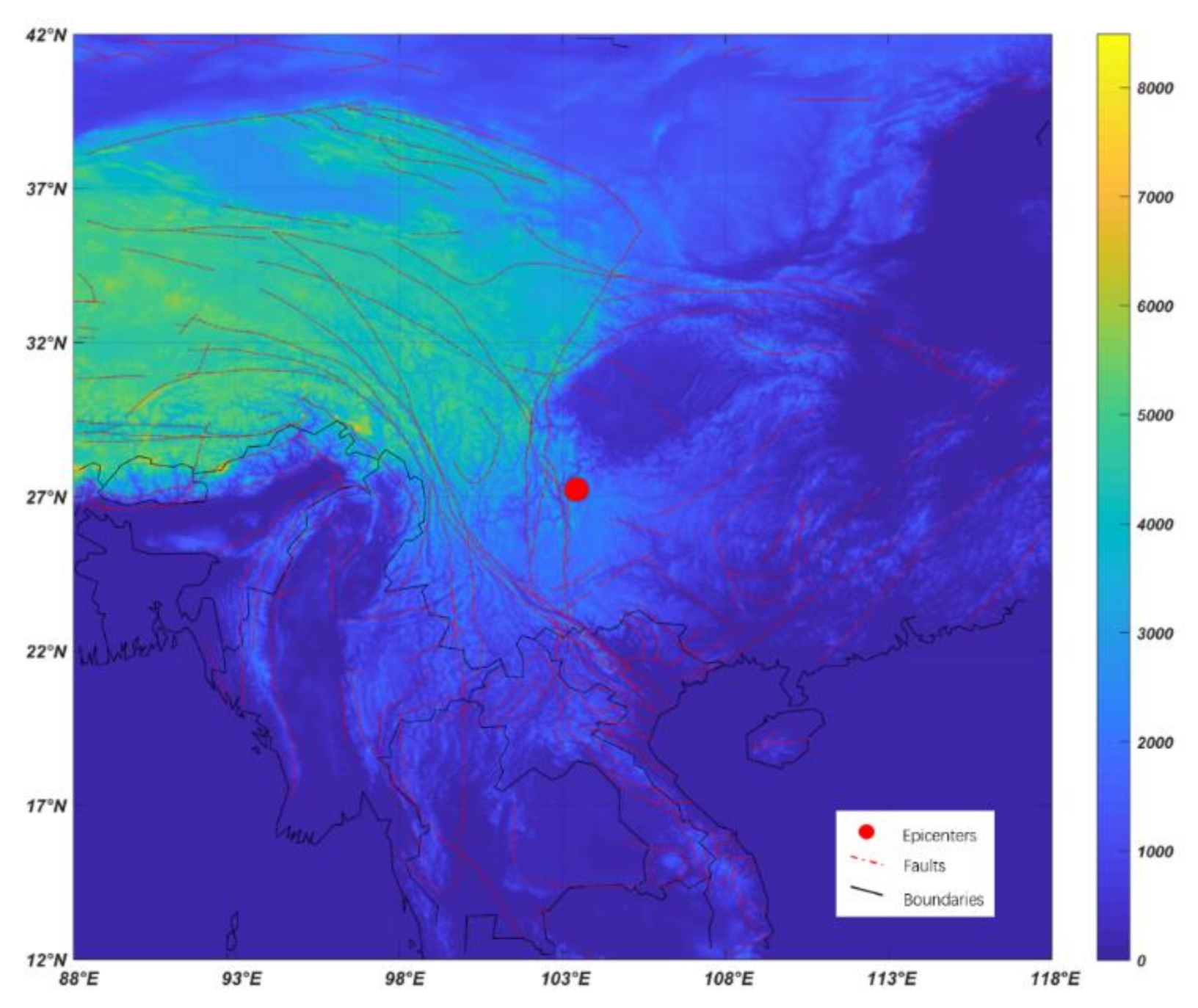
2. Tectonic Environment of Ludian Earthquake

As shown in Figure 1, an Mw 6.2 earthquake occurred on 3 August 2014, 8:30:13 (UTC) in Yunnan Province, China, as a result of shallow strike-slip faulting within the crust of the Eurasia plate, with its epicenter located at 27.245° N 103.427° E. In the following 20 days, there were 18 aftershocks near Ludian and Yongshan with magnitudes ranging from 4.0 to 5.0. Tectonics here are broadly controlled by the convergence of the India and Eurasia plates, which has driven the uplift of the Himalayas to the west of this earthquake, and caused the formation of numerous intraplate continental transform structures in the surrounding region, including the left-lateral Xiaojiang fault system. Local deformation rates in the region of this earthquake indicate as much as 10 mm/yr of left-lateral shear, and at the latitude of the 3 August 2014 event, India moves northwestward with respect to Eurasia at a rate of approximately 51 mm/yr (https://earthquake.usgs.gov/earthquakes (accessed on 1 January 2021)).

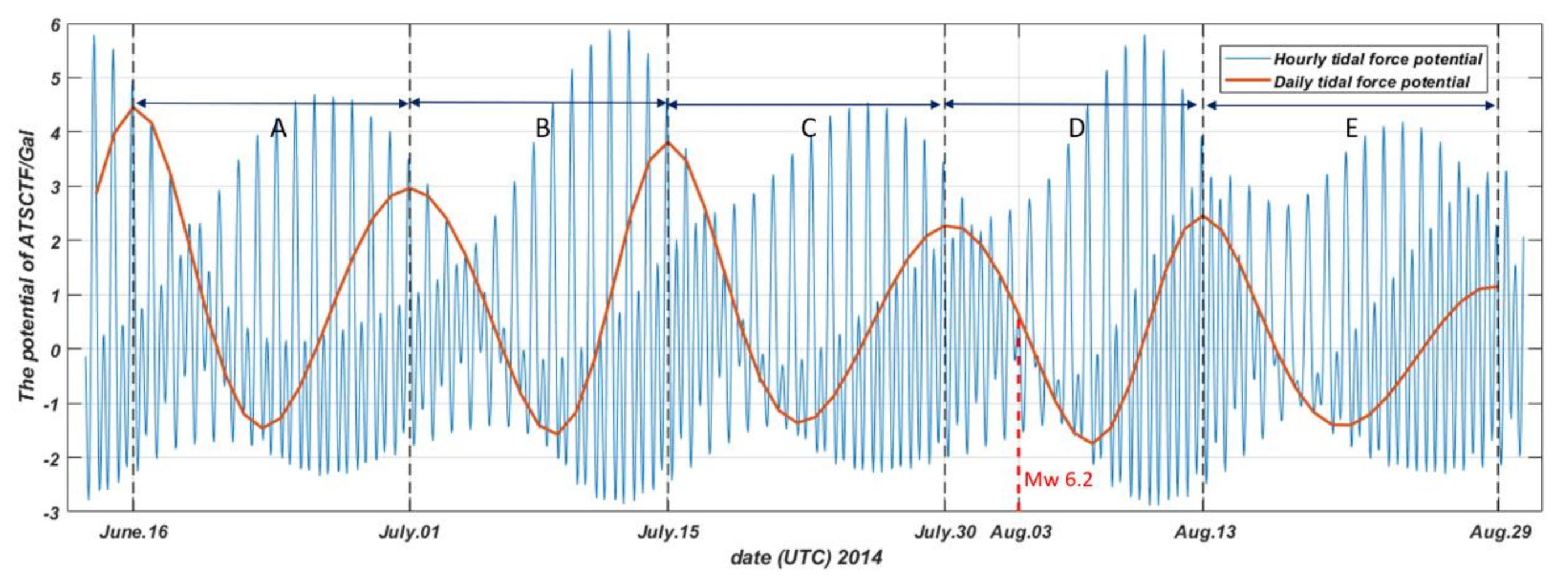
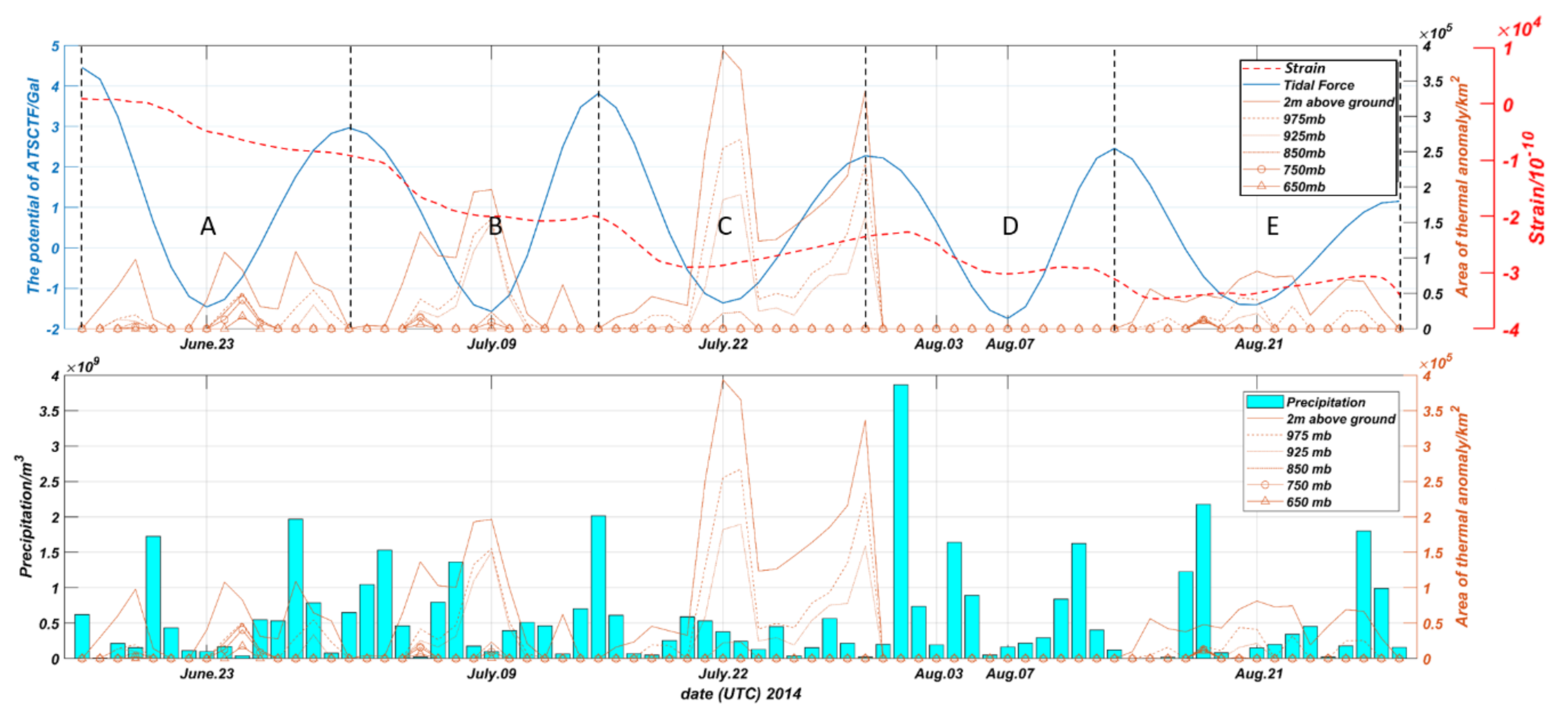
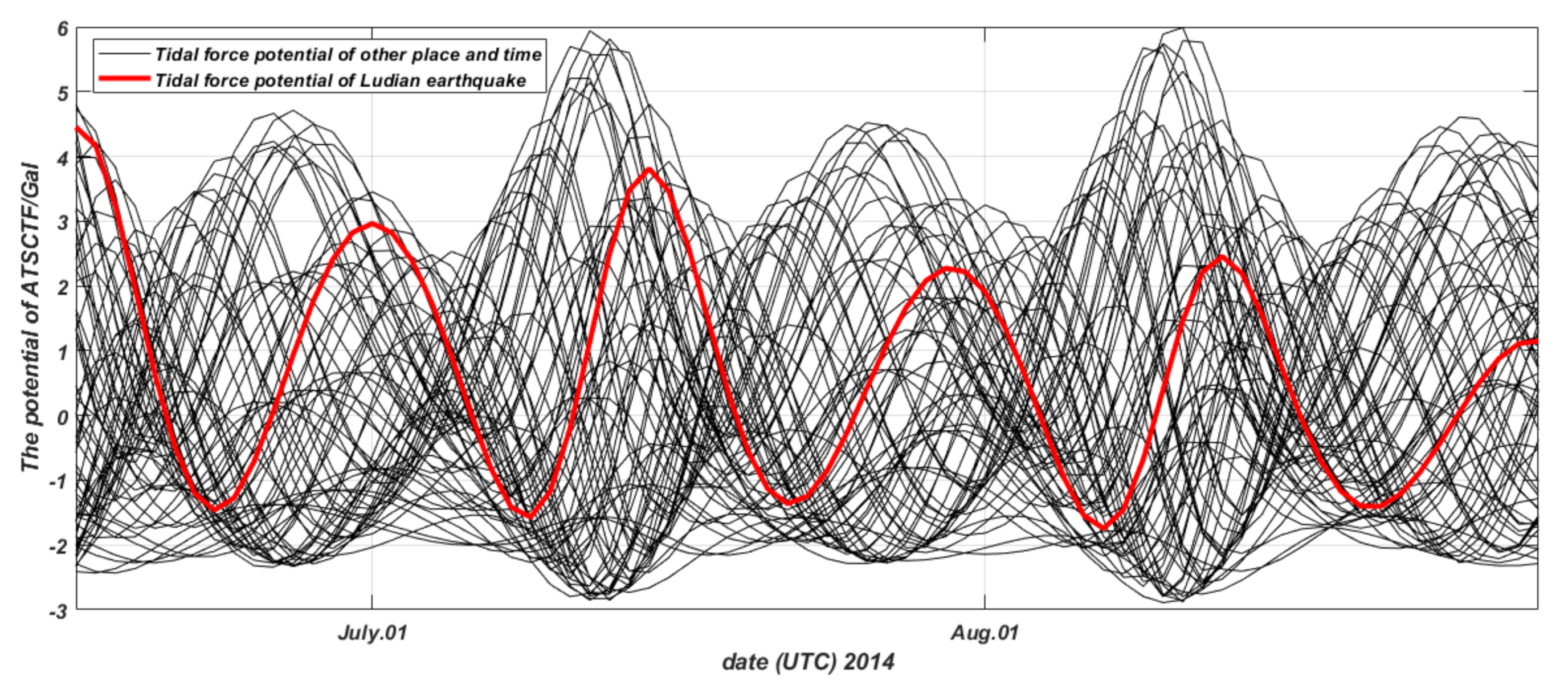
3. Change of Tidal Force and the TFFA Method

The differential gravitational forces provided by the Sun and the Moon lead to deformations on the surface of the Earth, along its radial axis, by up to 40 cm [31], and the tidal force has a significant influence on the stress within the Earth. As shown in Figure 2, we calculated the hourly tidal force potential at the hypocenter of the Ludian event, and the space derivative of the potential is the tidal stress. More information about how to calculate the tidal force potential can be found in References [30,34]. Beeler and Lockner [38] studied the correlation between the failure times and oscillating stress based on laboratory experiments in which faults are loaded to quasiperiodic failure by the combined action of a constant stressing rate, intended to simulate tectonic loading, and a small sinusoidal stress, analogous to the tidal force. They found that when the period of the oscillating stress is less than $t_n$, the correlation is not consistent with the threshold failure models, and the physical interpretation of $t_n$ is the duration of failure nucleation. Beeler and Lockner [38] indicated that “behavior at the higher frequencies is consistent with a second-order dependence of the fault strength on sliding rate, which determines the duration of nucleation and damps the response to stress change at frequencies greater than 1/$t_n$”, and $t_n$ exceeds the daily tidal period. Therefore, rather than the hourly tidal force potential, we considered the tidal force potential at a time scale of 24 h to study the Ludian earthquake. Therefore, we selected the tidal force potential at 8:30:13 (UTC) every day; 8:30:13 (UTC) is the time when the Ludian earthquake happened.

Ma et al. [34] proposed using the TFFA method to extract the thermal infrared (TIR) or thermal anomalies related to earthquakes. The first step of TFFA is to divide the data into different cycles according to the variation of daily tidal force potential. In TFFA, if the aiming earthquake occurred at the trough of sinusoidal tidal force, then each top of the sinusoidal variations is taken as the first day of each cycle. Similarly, if the earthquake occurred at the top, then the trough will be taken as the first day of each cycle. However, if the earthquake did not occur at the trough or the top, then the nearest preceding trough or top to the date of the earthquake is the candidate for the first day of each cycle. If the date of the earthquake is closer to the time of the trough rather than the top, we choose the trough, otherwise we choose the top. In this way, five fortnight cycles were based on the sinusoidal daily tidal force potential, as shown in Figure 2, each of them labeled as A, B, C, D, and E. As the red curve of Figure 2 shows, the Mw 6.2 earthquake occurred at the inflection point of cycle D. The five fortnight cycles we consider cover 16 June–1 July, 2–15 July, 16–30 July, 31 July–13 August, and 14–29 August. TFFA considers the first day of every cycle as the background reference, and $∆$T values are the air temperature data or TIR data of other days subtracted by their corresponding background; then, the variation of $∆$T is obtained. Finally, we need to set a threshold $\mathsf{\Phi }$ to identify the TIR or thermal anomalies, if $∆$T $\ge$ $\mathsf{\Phi }$, then it is regarded as an anomaly. The threshold is determined by the mean $\overline{∆\mathrm{T}}$ and standard deviation ${\sigma }_{∆\mathrm{T}}$ of $∆$T for the entire study area within the total study duration, and $\mathsf{\Phi }=\overline{∆\mathrm{T}}+3\ast {\sigma }_{∆\mathrm{T}}$.

4. Thermal Analysis

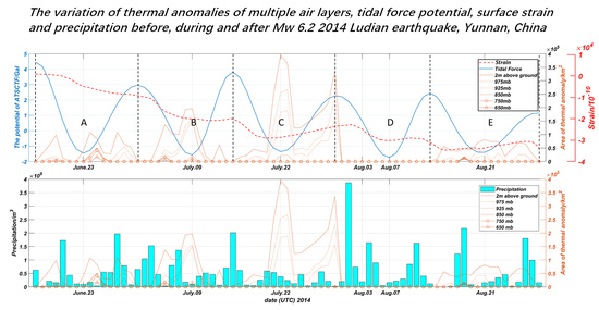
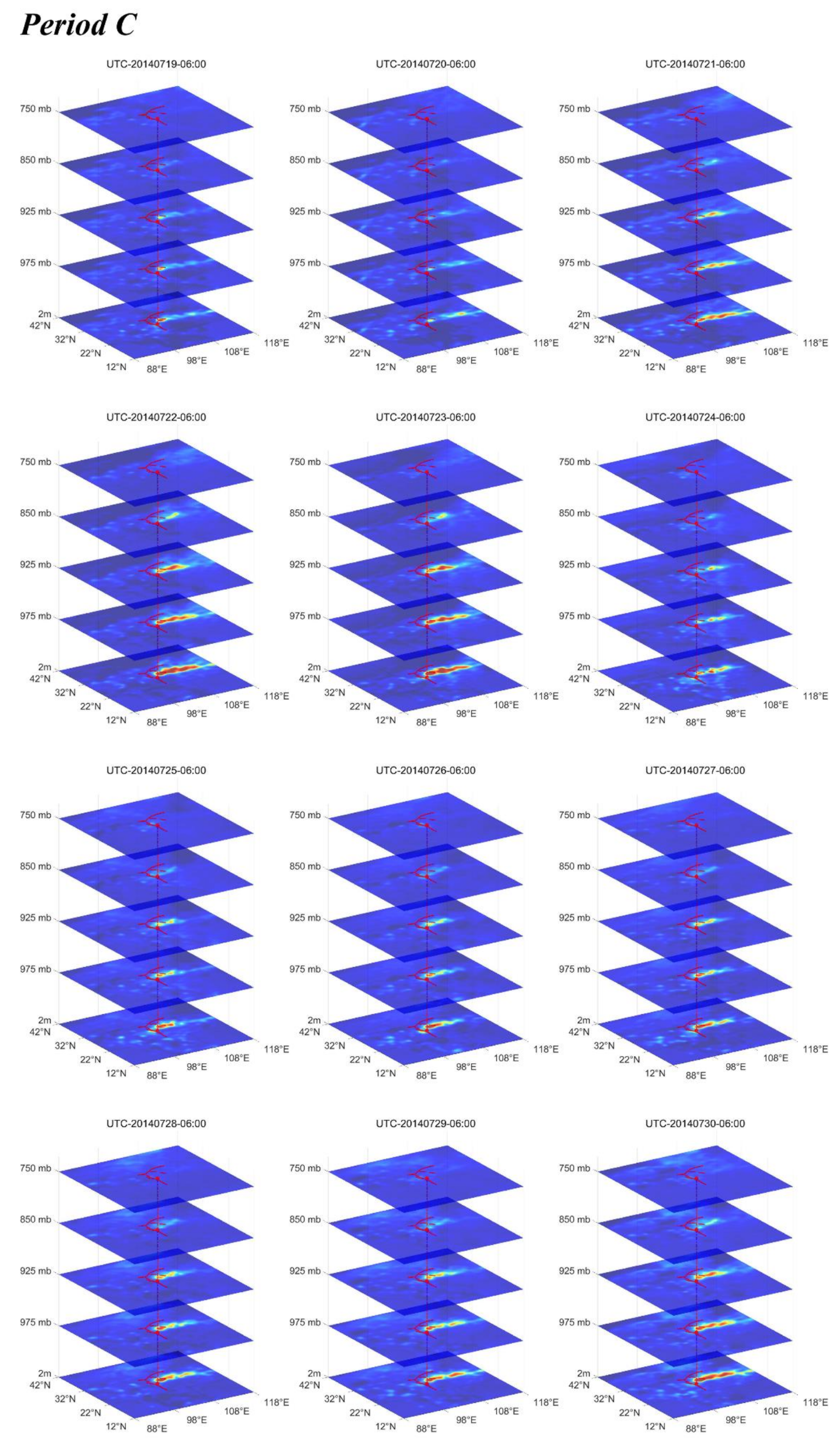
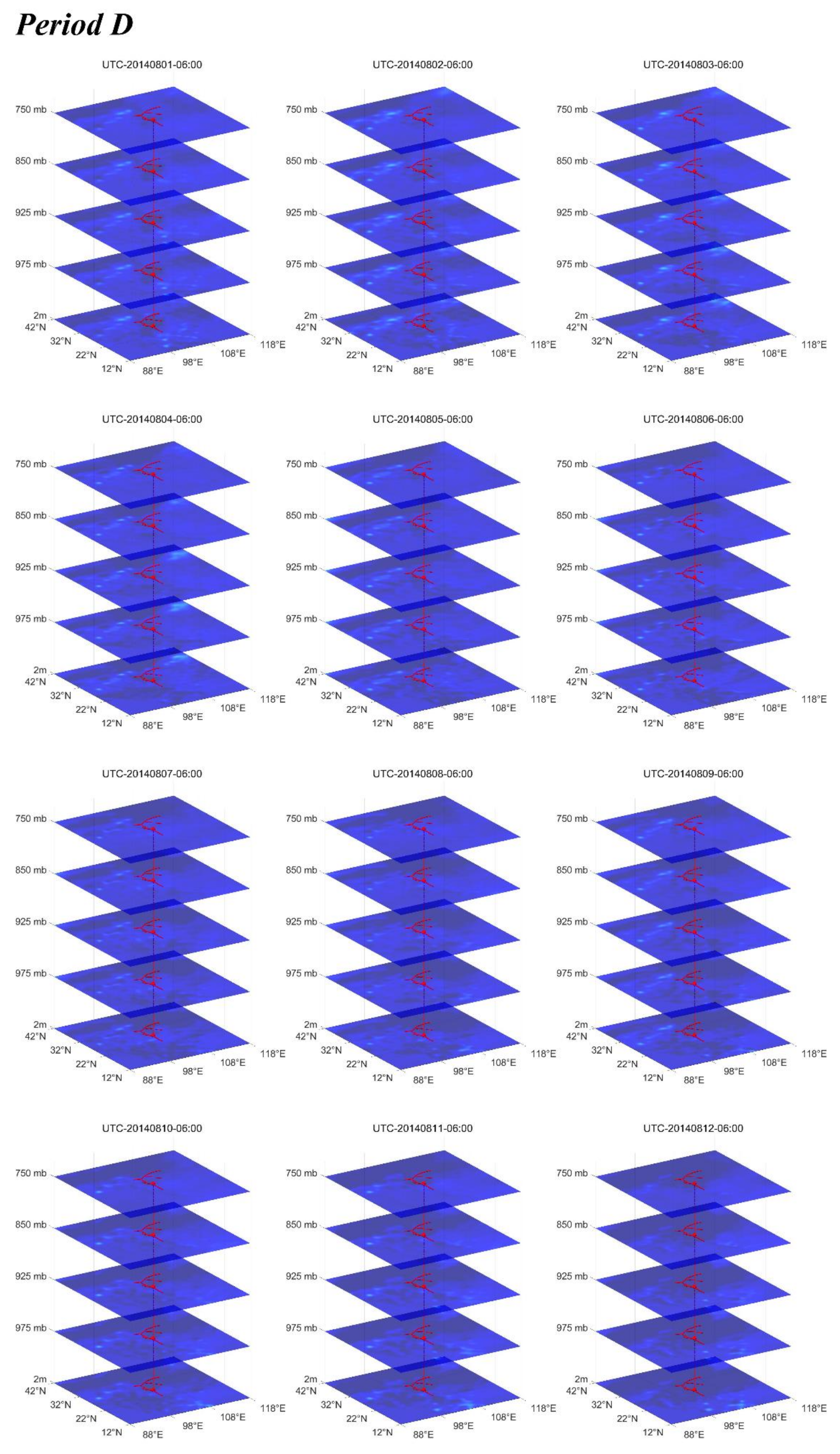
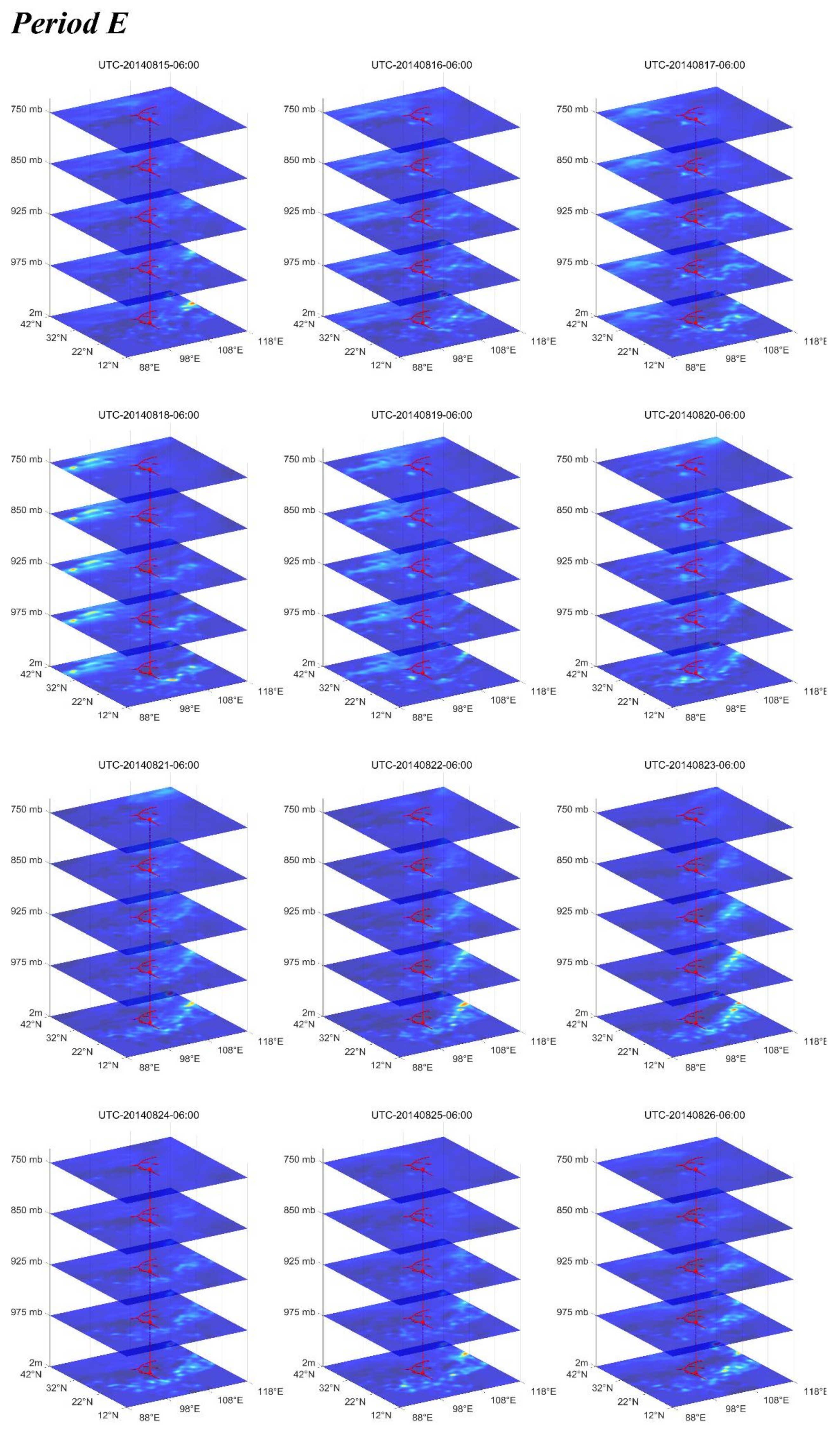
4.1. Multiple Layers of Air Temperature Evolution

The air temperature data are provided by NCEP, and it is a reanalysis product based on the Global Satellite Observation Data, Global Ground Observation Data, Integrated Ocean Data, Unmanned Aerial Vehicle (UAV) Observation Data, etc. The NCEP data are the most comprehensive, global reanalysis of meteorological data with 1° × 1° horizontal resolution, and this dataset provides temperature data for 26 isobaric surfaces [39]. Using the TFFA method, we can get the 3D variation of $∆$T. The multiple layers can help us to distinguish thermal anomalies caused by earthquakes from the ones influenced by a change of weather. If the air temperature increases first in the upper layer and is much larger than in the lower layer, it is obvious that this rise is not caused by land heating and earthquakes, but by the local weather [26]. In this study, we selected five layers of air temperature to show the occurrence, uplift, dissipation, and disappearance of thermal anomalies along the vertical direction. The five layers are located, from lowest to highest, 2 m above the ground, and then at altitudes corresponding to 975, 925, 850, and 750 mb pressure. The reason why isobaric layers started at 975 mb is that the altitude of epicenter is approximately 350 m, which corresponds to the isobaric surface with 976 mb, and the layers above 2 m above the ground should be with lower pressure, so we choose 975 mb as the starting isobaric layer. Moreover, five layers of air temperature ending at 750 mb are sufficient for presenting the vertical occurrence–dissipation–disappearance of the anomalies, and in this case there will be no more anomalies in the layers with pressure lower than 750 mb.

First, as shown in the Figure 3, we do a simple statistical analysis to determine the threshold $\mathsf{\Phi }$ to identify the anomalies. The negative skewness and positive kurtosis indicate that the distribution of $∆$T is not Gaussian, and the Jarque–Bera test also rejects the hypothesis that the distribution of $∆$T is Gaussian. In this case, it is shown in Figure 3 that $\mathsf{\Phi }=\overline{∆\mathrm{T}}+3\ast {\sigma }_{∆\mathrm{T}}\approx 11\mathrm{K}$. Furthermore, as shown in

Table 1. The distribution of $∆\mathrm{T}$.

Description	$\mathbf{Proportion}\mathbf{of}\mathbf{Qualified}\mathbf{∆}$$\mathbf{T}\mathbf{in}\mathbf{Total}\mathbf{∆}$
$∆\mathrm{T}\le \overline{∆\mathrm{T}}-3\ast {\sigma }_{∆\mathrm{T}}or∆\mathrm{T}\le -11\mathrm{K}$	1
$∆\mathrm{T}\le \overline{∆\mathrm{T}}-2\ast {\sigma }_{∆\mathrm{T}}or∆\mathrm{T}\le -8\mathrm{K}$	3.12
$∆\mathrm{T}\le \overline{∆\mathrm{T}}-{\sigma }_{∆\mathrm{T}}or∆\mathrm{T}\le -4\mathrm{K}$	12.06
$∆\mathrm{T}\ge \overline{∆\mathrm{T}}+{\sigma }_{∆\mathrm{T}}or∆\mathrm{T}\ge$4$\mathrm{K}$	12.83
$∆\mathrm{T}\ge \overline{∆\mathrm{T}}+2\ast {\sigma }_{∆\mathrm{T}}or∆\mathrm{T}\ge 8\mathrm{K}$	2.24
$∆\mathrm{T}\ge \overline{∆\mathrm{T}}+3\ast {\sigma }_{∆\mathrm{T}}or∆\mathrm{T}\ge 11\mathrm{K}$	0.57

, the proportion of $∆\mathrm{T}$ values that are greater than or equal to 11 K is only about 0.57%. From a statistical view, in this case, these $∆$T values that are larger than or equal to $\mathsf{\Phi }$ (11 K) are obviously highly anomalous signals.

As shown in Figure 4, there are thermal anomalies during cycles A, B, and C (as defined on Figure 2). All these anomalies appear in the lower layers, ascend, and then disappear in the high layers, so that they are identified as related to fault activity. We estimated the daily total precipitation near the epicenter (26°–28° N, 102°–104° E), which is shown in Figure 5 and at the bottom of Figure 6. Moreover, to quantitatively analyze the relation between thermal anomalies and other factors, we calculated the area of anomalies with $∆\mathrm{T}\ge 11 \mathrm{K}$ in different layers, as shown in Figure 6. As shown in Figure 4 and at the top of Figure 6, the maximum area and duration (A: from 24 to 26 June, 3 days; B: from 4 to 13 July, 10 days; C: from 19 to 30 July, 12 days) of each cycle were gradually increasing (C > B > A) when the earthquake was approaching. In each cycle before the earthquake, air temperature began to rise when the tidal force was quickly decreasing, reaching a peak at the troughs of the tidal force, attenuated, and disappeared when the tidal force was recovering. In periods A and B, the thermal anomalies disappeared after the trough of tidal force; however, the thermal anomalies in period C did not; these had attenuated compared to the last day, and there was another round of rising temperature until the end of the period. Based on the trend, we speculate that there should be some stronger thermal anomalies on 31 July, 1, 2, and 3 August, because seismotectonic stress is severe and approaching the critical breaking point. However, there are no thermal anomalies in period D. As shown in Figure 5, there was heavy rainfall around the epicenter on 1 August, which caused severe landslides (https://earthquake.usgs.gov/earthquakes (accessed on 1 January 2021)). The bottom of Figure 6 also indicates that rainfall around the epicenter is not frequent in these three months, but the strongest rainfall in this period occurred on 1 August, and the amount of precipitation was much larger than that of other days. The heavy regional rainfall may thus have concealed the potentially strong thermal anomalies in period D. There were thermal anomalies in period E as well. However, as shown in Figure 4E, their spatial distribution was scattered, and they were not persistent, so they were not identified as related to earthquakes.

We cannot directly get the seismotectonic stress before the earthquake, so we choose the surface strain data provided by the China Earthquake Administration (CEA), which are obtained by the model YRY-4 four-component borehole strain gauge, to reflect the variation of stress before and after the earthquake. These data are not open access. The strain data in this case were recorded by the Zhaotong station (27.4° N, 103.32° E), which is the closest station to the hypocenter; the sensor lies 45 m underground and far from the depth of the hypocenter (12 km). As shown in the upper plot of Figure 6, the negative strain indicates that the observation point is under compression and contraction during this period; moreover, the negative enhancement of strain indicates that the compression grew more intense from 16 June to 29 August. Chen et al. [40] conducted an experiment to study the relation between stress–strain and variation of temperature, and the results showed that the surface strain is positively correlated to the strain strength. However, as shown in Figure 4 and at the top of Figure 6, there were no thermal anomalies after the earthquake when the strain was still negative and increasing. One possible hypothesis that explains this contradiction is that the deformation of surface ground (45 m) cannot reflect the variation of stress of deep layers near the hypocenters. That is, the elastic deformation of the surface ground is not the source of the thermal anomalies in this case; if it were, then there would be more thermal anomalies in periods D and E after the earthquakes. Moreover, the variation of stress or strain around the hypocenter, where there might be a source creating the thermal anomalies, is different from the strain at the observation point (45 m). The mechanism of thermal anomalies created by earthquakes in the natural environment needs further study.

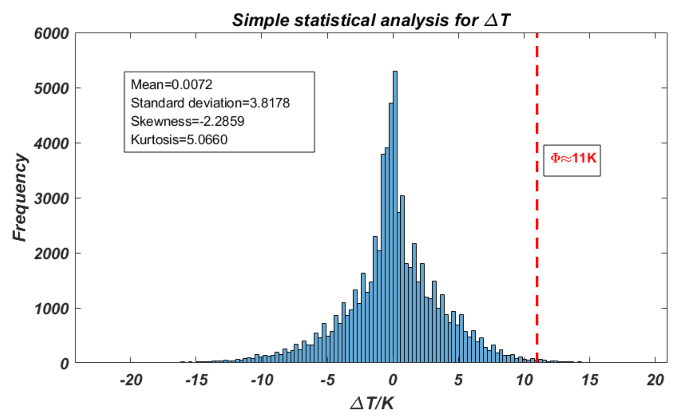
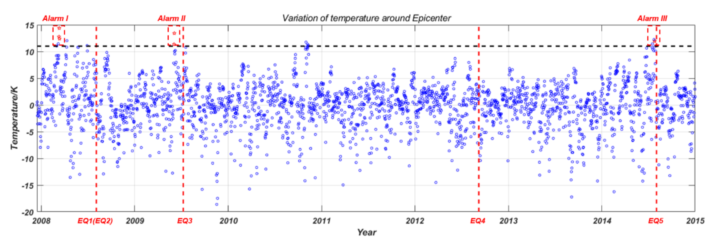
4.2. Significance Test for Thermal Anomalies

We introduce a significance test to prove whether or not the observed thermal anomalies are related to the Ludian earthquake. The variations of fortnight tidal force potential for different hypocenters and times differ much from each other. As shown in Figure 7, we also calculated the tidal force potential at several locations {Longitude, Latitude, Depth|$\left\{\mathrm{Longtitude},\mathrm{Latitude},\mathrm{Depth}\right\}$ and $\mathrm{Time}$, using $\mathrm{Longtitude}=\left\{{88}^{°}\mathrm{E},{103}^{°}\mathrm{E},{118}^{°}\mathrm{E}\right\}$, $\mathrm{Latitude}=\left\{{12}^{°}\mathrm{N},{27}^{°}\mathrm{N},{42}^{°}\mathrm{N}\right\}$, $\mathrm{Depth}=12\mathrm{km}$ and $\mathrm{Time}=\left\{0,4,8,12,16,20\left(\mathrm{hour},\mathrm{UTC}\right)\right\}$. Figure 7 indicates that the backgrounds indicated by the TFFA method are spatially and temporally varying. This shows that the TFFA will be ineffective for areas far from the hypocenters and for different times when performing long-term statistical studies. Therefore, we selected the area around the epicenter (27°–28° N 103°–104° E) as the area of interest, and the average of $∆\mathrm{T}$ for these four pixels from December 2007 to December 2014 was based on the TFFA method. We then set a relative intensity rule and a temporal persistence rule for extracting thermal anomalies:

• Relative intensity rule—similar to the thermal anomalies of the Ludian earthquake, we set 11 K as the threshold;
• Temporal persistence rule—unlike some thermal anomalies caused by short-term and instantaneous change of weather, the thermal anomalies of earthquakes should be extended in time, so that the seismic thermal anomalies should appear for at least two consecutive days.

In that way, we extracted three thermal anomalies, which are Alarm I, II, and III, as shown in Figure 8. We then searched for the earthquakes that are potentially related to those thermal anomalies. According to the former cases [26,34,35,36,37], we found that there is a strong spatial–temporal correlation between earthquakes with magnitude ≥5.5 and thermal anomalies extracted by the TFFA method. The latest thermal anomalies extracted by TFFA always occur within two weeks—i.e., a cycle of tidal force potential—before earthquakes, and the spatial distances between the thermal anomalies and earthquakes are smaller than or equal to $2°$. With these empirical conclusions, we selected earthquakes that occurred within 25°–30° N, 101°–106° E with magnitude ≥5.5 from December 2007 to December 2014 for this test. There are five such earthquakes, shown in

Table 2. Earthquakes occurring within 25°–30° N, 101°–106° E with magnitude ≥ 5.5 from December 2007 to December 2014; EQ5 is the Ludian earthquake.

	Time	$\mathbf{Latitude}(°\mathbf{N})$	$\mathbf{Longitude}(°\mathbf{E})$	Depth (km)	Mag (Mw)
EQ1	30-08-2008	26.24	101.89	11	6
EQ2	31-08-2008	26.23	101.97	10	5.6
EQ3	09-07-2009	25.63	101.10	7	5.7
EQ4	07-09-2012	27.58	103.98	10	5.5
EQ5	03-08-2014	27.24	103.42	12	6.2

and as EQ1–EQ5 in the Figure 8.

In this study, the performance of thermal anomalies used as precursors is compared with random guessing. Random guessing means that there is no relation between earthquakes and thermal anomalies, and that they will occur at any time with equal probability. First, we get the prior probability that thermal anomalies at any time will correspond to earthquakes, assuming that the thermal anomalies are independent of earthquakes. For determining the correspondence between earthquakes and thermal anomalies, we set a temporal window of k days. For example, if the alarm A appears within k days before EQ1, the alarm A is judged to be related to EQ1. In return, using this temporal window and the earthquake catalog, we can determine a group of days such that, if these thermal anomalies occur (even randomly) on these days, they will correspond to earthquakes. For earthquake i occurring at $t_i$, if alarms occur at times {$t_i-k,t_i-k+1,\dots ,t_i-1,t_i$}, they will correspond to earthquake i and these alarms are regarded as true positives. Similarly, we can obtain N groups of days for all the N earthquakes, and $\mathsf{\Phi }$ is the union of these N groups of days. We can then get the prior probability $\mathcal{P}$ for the alarms as follows:

$$\mathcal{P}=number of days of \mathsf{\Phi }/number of days of study duration$$

(1)

The number of true positives for alarms follows a binomial distribution:

$$B(h|N_A,\mathcal{P})=\left(\begin{array}{c}{N}_A\\ h\end{array}\right){\left(\mathcal{P}\right)}^h{\left(1-\mathcal{P}\right)}^{N_A-h}$$

(2)

where h is the number of hit events or the number of true positives, and $N_A$ is the total number of alarms. Finally, we can get the $\mathit{P}\left(h\le H\le N_A\right)$ as follows:

$$\mathit{P}\left(h\le H\le N_A\right)={\displaystyle \sum }_{n=h}^{N_A}B(n|N_A,\mathcal{P})$$

(3)

Our null hypothesis is that thermal anomalies are not related to earthquakes. If $\mathit{P}\left(h\le H\le N_A\right)<\alpha$, where $\alpha$ is the significance level, and if $\alpha <<1$, we reject the null hypothesis, and thermal anomalies are related to earthquakes. In this study, we set $\alpha =0.05$. For the temporal window k, as is shown in Figure 4a, the earliest thermal anomalies regarded to be related to the Ludian earthquake appeared on 24 June, i.e., 40 days before the event. Therefore, we set k = 40 and P-value = 0.0112 < 0.05. We then reject the null hypothesis, and the long-term thermal anomalies around the epicenter of Ludian earthquake extracted by TFFA are related to earthquakes.

5. Discussion

Unlike the thermal infrared remote sensing data, the air temperature data provided by NCEP are not affected by clouds. When the area is obscured by clouds, it is impossible to extract thermal infrared anomalies caused by earthquakes, because thermal infrared data record cloud top radiation rather than land surface radiation. Moreover, the statistical methods for extracting thermal anomalies requires a lot of data processing, and the lack of good data will lead to bad and unreliable results. Figure 9 shows the cloud map provided by FY-2. The results show that the epicenter and even the whole study area were covered by clouds when there was a thermal anomaly under the clouds. In other words, it would have been impossible to get reliable, persistent, stable, and obvious thermal anomalies in the case of the Ludian earthquake using thermal infrared remote sensing data. It is concluded that, compared to thermal infrared data, air temperature data provided by NCEP have a huge advantage for monitoring the pre-earthquake temperature variation in cloudy areas. Strong cooling weather such as heavy rainfall and blizzard [41], however, can also hide the thermal anomalies, and how to extract the thermal anomalies before earthquakes under such weather needs further study. There is another huge limitation for the TFFA, because the key point of this method is the variation of tidal force potential at the hypocenter, but the information about the hypocenter is known only after the earthquake occurs. Therefore, this method is more suitable for studying the relationship between thermal anomalies and earthquakes, but cannot be used for earthquake prediction.

6. Conclusions

During cycles A, B, and C, all of the thermal anomalies are located on or near epicenters, and they generate from the bottom, spread upward, and disappear in the top layers. The vertical characteristic of those thermal anomalies is consistent with the results of the Mw 5.7 Jiujiang earthquake, and coincide with the principle of atmospheric thermal dynamic diffusion along the vertical: air heated by land, uplifted by heat flux, cooled and dissipated in the sky [26]. From period A to C, with the approaching earthquake, the thermal anomalies within each cycle become significantly more intense; moreover, the variation of the thermal anomaly within each cycle coincides with that of the tidal force potential. The thermal anomalies begin to rise at the quickly declining phase, reach a peak at troughs, and attenuate at the recovery phase. Based on the high spatial–temporal correlation between thermal anomalies and the Ludian earthquake, high consistency between spatial–temporal variation of thermal anomalies and tidal force potential, and the strong evidence provided by the significance test, it can be concluded that the thermal anomalies in periods A, B, and C are caused by the Ludian earthquake.

As shown in Figure 2, the variation of the tidal force potential is quasiperiodic. However, no earthquakes occurred during the similar phases at other times. Based on the opinion that the variance of air temperature can reflect the change of state of seismotectonic stress [26], we can propose that the relationship between the state of seismotectonic stress of cycles A, B, and C is as follows: C > B > A. In spite of the fact that there is energy accumulation caused by the tectonic displacement during periods A and B, it is released rapidly as the tidal force potential recovers. In period C, there are two rounds of rising air temperature. That means that the state of seismotectonic stress in period C increases until the critical breaking point of rocks, and then the earthquake occurs. The increasing seismotectonic stress during each cycle and the fact that no earthquake occurs during the similar phase of tidal force potential indicates that the state of seismotectonic stress is the decisive factor for triggering earthquakes, not the tidal force potential [26]. The Ludian earthquake is a good example to show the relationship between an earthquake, the tidal force potential, thermal anomalies (air temperature), and the state of seismotectonic stress; the tidal force potential can change the state of seismotectonic stress, which can change the local air temperature. However, earthquakes occur only when the seismotectonic stress reaches the critical breaking point of rocks. However, under the same tidal force potential, it is unknown what caused the different stress states in different periods, and what made the energy accumulation in period C much stronger than periods A and B. Exploring the potential factor is of great significance to the study of the mechanism of the Ludian earthquake and earthquake prediction.

References

1. Bi, Y.; Wu, S.; Xiong, P.; Shen, X. A Comparative Analysis for Detecting Seismic Anomalies in Data Sequences of Outgoing Longwave Radiation; Springer: Berlin/Heidelberg, Germany, 2009. [Google Scholar]
2. Carreno, E.; Capote, R.; Yague, A.; Tordesillas, J.M.; Lopez, M.M.; Ardizone, J.; Suarez, A.; Lzquierdo, A.; Tsige, M.; Martinez, J.; et al. Observations of Thermal Anomaly Associated to Seismic Activity from Remote Sensing; General Assembly of European Seismology Commission: Lisbon, Portugal, 2001; pp. 10–15. [Google Scholar]
3. Saraf, A.K.; Choudhury, S. Cover: Satellite detects surface thermal anomalies associated with the Algerian earthquakes of May 2003. Int. J. Remote Sens. 2005, 26, 2705–2713. [Google Scholar] [CrossRef]
4. Jing, F.; Shen, X.H.; Kang, C.L.; Xiong, P. Variations of multi-parameter observations in atmosphere related to earthquake. Nat. Hazards Earth Syst. Sci. 2013, 13, 27–33. [Google Scholar] [CrossRef] [Green Version]
5. Lu, X.; Meng, Q.Y.; Gu, X.F.; Zhang, X.D.; Xie, T.; Geng, F. Thermal Infrared Anomalies Associated with Multi-year Earthquakes in the Tibet Region Based on China’s FY-2E Satellite Data. Adv. Space Res. 2016, 58, 989–1001. [Google Scholar] [CrossRef]
6. Ouzounov, D.; Freund, F. Mid-infrared emission prior to strong earthquakes analyzed by remote sensing data. Adv. Space Res. 2004, 33, 268–273. [Google Scholar] [CrossRef]
7. Ouzounov, D.; Liu, D.; Chunli, K.; Cervone, G.; Kafatos, M.; Taylor, P. Outgoing long wave radiation variability from IR satellite data prior to major earthquakes. Tectonophysics 2007, 431, 211–220. [Google Scholar] [CrossRef]
8. Panda, S.K.; Choudhury, S.; Saraf, A.K.; Das, J.D. MODIS land surface temperature data detects thermal anomaly preceding 8 October 2005 Kashmir earthquake. Int. J. Remote Sens. 2007, 28, 4587–4596. [Google Scholar] [CrossRef]
9. Qin, K.; Wu, L.; Zheng, S.; Liu, S. A Deviation-Time-Space-Thermal (DTS-T) Method for Global Earth Observation System of Systems (GEOSS)-Based Earthquake Anomaly Recognition: Criterions and Quantify Indices. Remote Sens. 2013, 5, 5143–5151. [Google Scholar] [CrossRef] [Green Version]
10. Saraf, A.K.; Choudhury, S. Thermal remote sensing technique in the study of pre-earthquake thermal anomalies. J. Ind. Geophys. Union 2005, 9, 197–207. [Google Scholar]
11. Saraf, A.K.; Choudhury, S. Cover: NOAA-AVHRR detects thermal anomaly associated with the 26 January 2001 Bhuj earthquake, Gujarat, India. Int. J. Remote Sens. 2005, 26, 1065–1073. [Google Scholar] [CrossRef]
12. Saraf, A.K.; Rawat, V.; Choudhury, S.; Dasgupta, S.; Das, J. Advances in understanding of the mechanism for generation of earthquake thermal precursors detected by satellites. Int. J. Appl. Earth Obs. Geoinf. 2009, 11, 373–379. [Google Scholar] [CrossRef]
13. Tronin, A.A.; Hayakawa, M.; Molchanov, O.A. Thermal IR satellite data application for earthquake research in Japan and China. J. Geodyn. 2002, 33, 519–534. [Google Scholar] [CrossRef]
14. Tronin, A.A. Satellite thermal survey a new tool for the study of seismoactive regions. Int. J. Remote Sens. 1996, 17, 1439–1455. [Google Scholar] [CrossRef]
15. Zhang, Y.; Guo, X.; Zhong, M.; Shen, W.; Li, W.; He, B. Wenchuan earthquake: Brightness temperature changes from satellite infrared information. Sci. Bull. 2010, 55, 1917–1924. [Google Scholar] [CrossRef]
16. Aliano, C.; Corrado, R.; Filizzola, C.; Pergola, N.; Tramutoli, V. Robust Satellite Techniques (RST) for Seismically Active Areas Monitoring: The Case of 21st May, 2003 Boumerdes/Thenia (Algeria) Earthquake. In Proceedings of the 2007 International Workshop on the Analysis of Multi-temporal Remote Sensing Images, Leuven, Belgium, 18–20 July 2007. [Google Scholar]
17. Aliano, C.; Corrado, R.; Filizzola, C.; Genzano, N.; Lanorte, V.; Mazzeo, G.; Pergola, N.; Tramutoli, V. Robust Satellite Techniques (RST) for monitoring thermal anomalies in seismically active areas. In Proceedings of the 2009 IEEE International Geoscience and Remote Sensing Symposium, Cape Town, South Africa, 12–17 July 2009. [Google Scholar]
18. Bellaoui, M.; Hassini, A.; Kada, B. Pre-seismic Anomalies in Remotely Sensed Land Surface Temperature measurements: The Case Study of 2003 Boumerdes Earthquake. Adv. Space Res. 2017, 59, 2645–2657. [Google Scholar] [CrossRef]
19. Boudin, F.; Bernard, P.; Esnoult, M.F.; Olcay, M.; Tassera, C.; Aissaoui, E.M.; Nercessian, A.; Vilotte, J.P. Evidence for slow slip events preceeding the M8, April 1rst, 2014 Pisagua Earthquake (Chile), from an underground, long base hydrostatic tiltmeter. In AGU Fall Meeting Abstracts; American Geophysical Union: San Francisco, CA, USA, 2014. [Google Scholar]
20. Genzano, N.; Aliano, C.; Corrado, R.; Filizzola, C.; Lisi, M.; Mazzeo, G.; Paciello, R.; Pergola, N.; Tramutoli, V. RST analysis of MSG-SEVIRI TIR radiances at the time of the Abruzzo 6 April 2009 earthquake. Nat. Hazards Earth Syst. Sci. Discuss. 2009, 9, 2073–2084. [Google Scholar] [CrossRef]
21. Genzano, N.; Corrado, R.; Coviello, I.; Grimaldi, C.S.; Filizzola, C.; Lacava, T.; Lisi, M.; Marchese, F.; Mazzeo, G.; Paciello, R.; et al. A multi-sensors analysis of RST-based thermal anomalies in the case of the Abruzzo earthquake. In Proceedings of the 2010 IEEE International Geoscience and Remote Sensing Symposium, Honolulu, HI, USA, 25–30 July 2010. [Google Scholar]
22. Lisi, M.; Filizzola, C.; Genzano, N.; Grimaldi, C.S.; Lacava, T.; Marchese, F.; Mazzeo, G.; Pergola, N.; Tramutoli, V. A study on the Abruzzo 6 April 2009 earthquake by applying the RST approach to 15 years of AVHRR TIR observations. Nat. Hazards Earth System Sci. 2010, 10, 395–406. [Google Scholar] [CrossRef]
23. Lisi, M.; Filizzola, C.; Genzano, N.; Paciello, R.; Pergola, N.; Tramutoli, V. Reducing atmospheric noise in RST analysis of TIR satellite radiances for earthquakes prone areas satellite monitoring. Phys. Chem. Earth Parts A/B/C 2015, 85, 87–97. [Google Scholar] [CrossRef]
24. Pergola, N.; Aliano, C.; Coviello, I.; Filizzola, C.; Genzano, N.; Lacava, T.; Lisi, M.; Mazzeo, G.; Tramutoli, V. Using RST approach and EOS-MODIS radiances for monitoring seismically active regions: A study on the 6 April 2009 Abruzzo earthquake. Nat. Hazards Earth System Sci. 2010, 10, 239–249. [Google Scholar] [CrossRef]
25. Sannazzaro, F.; Filizzola, C.; Marchese, F.; Corrado, R.; Paciello, R.; Mazzeo, G.; Pergola, N.; Tramutoli, V. Identification of dust outbreaks on infrared MSG-SEVIRI data by using a Robust Satellite Technique (RST). Acta Astronaut. 2014, 93, 64–70. [Google Scholar] [CrossRef]
26. Weiyu, M.; Xuedong, Z.; Liu, J.; Yao, Q.; Zhou, B.; Yue, C.; Kang, C.; Lu, X. Influences of multiple layers of air temperature differences on tidal forces and tectonic stress before, during and after the Jiujiang earthquake. Remote Sens. Environ. 2018, 210, 159–165. [Google Scholar] [CrossRef]
27. Blackett, M.; Wooster, M.J.; Malamud, B.D. Exploring land surface temperature earthquake precursors: A focus on the Gujarat (India) earthquake of 2001. Geophys. Res. Lett. 2011, 38, L15303. [Google Scholar] [CrossRef]
28. Zhang, Y.; Qingyan, M. A statistical analysis of TIR anomalies extracted by RSTs in relation to an earthquake in the Sichuan area using MODIS LST data. Nat. Hazards Earth Syst. Sci. 2019, 19, 535–549. [Google Scholar] [CrossRef] [Green Version]
29. Cochran, E.S.; Vidale, J.E.; Tanaka, S. Earth Tides Can Trigger Shallow Thrust Fault Earthquakes. Science 2004, 306, 1164–1166. [Google Scholar] [CrossRef] [Green Version]
30. Tanaka, S.; Ohtake, M.; Sato, H. Spatio-temporal variation of the tidal triggering effect on earthquake occurrence associated with the 1982 South Tonga earthquake of Mw 7.5. Geophys. Res. Lett. 2002, 29, 3-1–3-4. [Google Scholar] [CrossRef]
31. Heaton, T.H. Tidal Triggering of Earthquakes. Geophys. J. R. Astron. Soc. 1975, 43, 307–326. [Google Scholar] [CrossRef] [Green Version]
32. Kilston, S.; Knopoff, L. Lunar–solar periodicities of large earthquakes in southern California. Nature 1983, 304, 21–25. [Google Scholar] [CrossRef]
33. Mcnutt, S.R.; Beavan, R.J. Volcanic earthquakes at Pavlof Volcano correlated with the solid earth tide. Nature 1981, 294, 615–618. [Google Scholar] [CrossRef]
34. Ma, W.Y.; Wang, H.; Li, F.S.; Ma, W.M. Relation between the celestial tide-generating stress and the temperature variations of the Abruzzo M = 6.3 Earthquake in April 2009. Nat. Hazards Earth System Sci. 2012, 12, 819–827. [Google Scholar] [CrossRef] [Green Version]
35. Yan, Z.; Chunli, K.; Weiyu, M.; Qi, Y. The Change in Outgoing Long-wave Radiation before the Ludian Ms6.5 Earthquake Based on Tidal Force Niche Cycles. Earthq. Res. China 2017, 3, 422–430. [Google Scholar]
36. Zhang, X.; Kang, C.; Ma, W.; Ren, J.; Wang, Y. Study on thermal anomalies of earthquake process by using tidal-force and outgoing-longwave-radiation. Therm. Sci. 2017, 22, 153. [Google Scholar] [CrossRef]
37. Ma, W.; Kong, X.; Kang, C.; Zhong, X.; Wu, H.; Zhan, X.; Joshi, M. Research on the changes of the tidal force and the air temperature in the atmosphere of Lushan (China) MS7.0 earthquake. Therm. Sci. 2015, 19, 148. [Google Scholar] [CrossRef]
38. Beeler, N.; Lockner, D. Why earthquakes correlate weakly with the solid Earth tides: Effects of periodic stress on the rate and probability of earthquake occurrence. J. Geophys. Res. 2003, 108. [Google Scholar] [CrossRef] [Green Version]
39. Kistler, R.; Kalnay, E.; Collins, W.; Saha, S.; White, G.; Woollen, J.; Chelliah, M.; Ebisuzaki, W.; Kanamitsu, M.; Kousky, V.; et al. The NCEP-NCAR 50-Year Reanalysis: Monthly Means CD-ROM and Documentation. Bull. Am. Meteorol. Soc. 2001, 82, 247–268. [Google Scholar] [CrossRef]
40. Chen, S.; Liu, L.; Liu, P.; Ma, J.; Chen, G. Theoretical and experimental study on relationship between stress-strain and temperature variation. Sci. China Ser. D Earth Sci. 2009, 39, 1446–1455. [Google Scholar] [CrossRef]
41. Meng, Q.; Zhang, Y. Discovery of Spatial-temporal Causal Interactions between Thermal and Methane Anomalies Associated with the Wenchuan Earthquake. Eur. Phys. J. Spec. Top. 2021, 230, 247–261. [Google Scholar] [CrossRef]
Figure 1. Distribution of faults in the study area (12–42° N, 88–118° E). The red point is the epicenter, and right legend is elevation (m).
Remotesensing 13 00884 g001
Figure 2. The change of additive tectonic stress from the celestial tide-generating force (ATSCTF) or tidal force potential for the Ludian earthquake. The red curve is the daily tidal force potential at 8:30:13 (UTC).
Remotesensing 13 00884 g002
Figure 3. The histrogram of T in study area from 16 June to 29 August. The mean, standard deviation, skewness, kurtosis, and Φ are also shown in this plot.
Remotesensing 13 00884 g003
Figure 4. Variation of multiple layers of air temperature for cycles (AE). The red point is the epicenter and the red lines are the faults. Column and row of each subplot is latitude and longitude, respectively. The z-axis is the layer with different air pressure, and the reason why we do not use the altitudes is that layers with the same pressure are not at the same altitudes. For the balance and beauty of the legend, parts from −18 to −5 K are marked with the same color of −5 K, and they are not presented in the legend.
Remotesensing 13 00884 g004aRemotesensing 13 00884 g004bRemotesensing 13 00884 g004cRemotesensing 13 00884 g004dRemotesensing 13 00884 g004e
Figure 5. The precipitation from 29 July to 3 August. The red point is the epicenter and the right legend is the precipitation (mm).
Remotesensing 13 00884 g005
Figure 6. The upper plot compares the anomalous area of several layers, the tidal force potential, and the surface strain of model YRY-4 four-component borehole strain gauge located at the Zhaotong observation station, while the bottom plot compares the area of the thermal anomaly and the precipitation.
Remotesensing 13 00884 g006
Figure 7. Variations of tidal force potential for different locations and times. The red line is the result for the Ludian earthquake location.
Remotesensing 13 00884 g007
Figure 8. Long-term variation of temperature around the epicenter area (27°–28° N, 103°–104° E).
Remotesensing 13 00884 g008
Figure 9. Cloud maps for the days of thermal anomalies.
Remotesensing 13 00884 g009