
Improving Co-Registration for Sentinel-1 SAR and Sentinel-2 Optical Images


Abstract
:
1. Introduction
- (1)
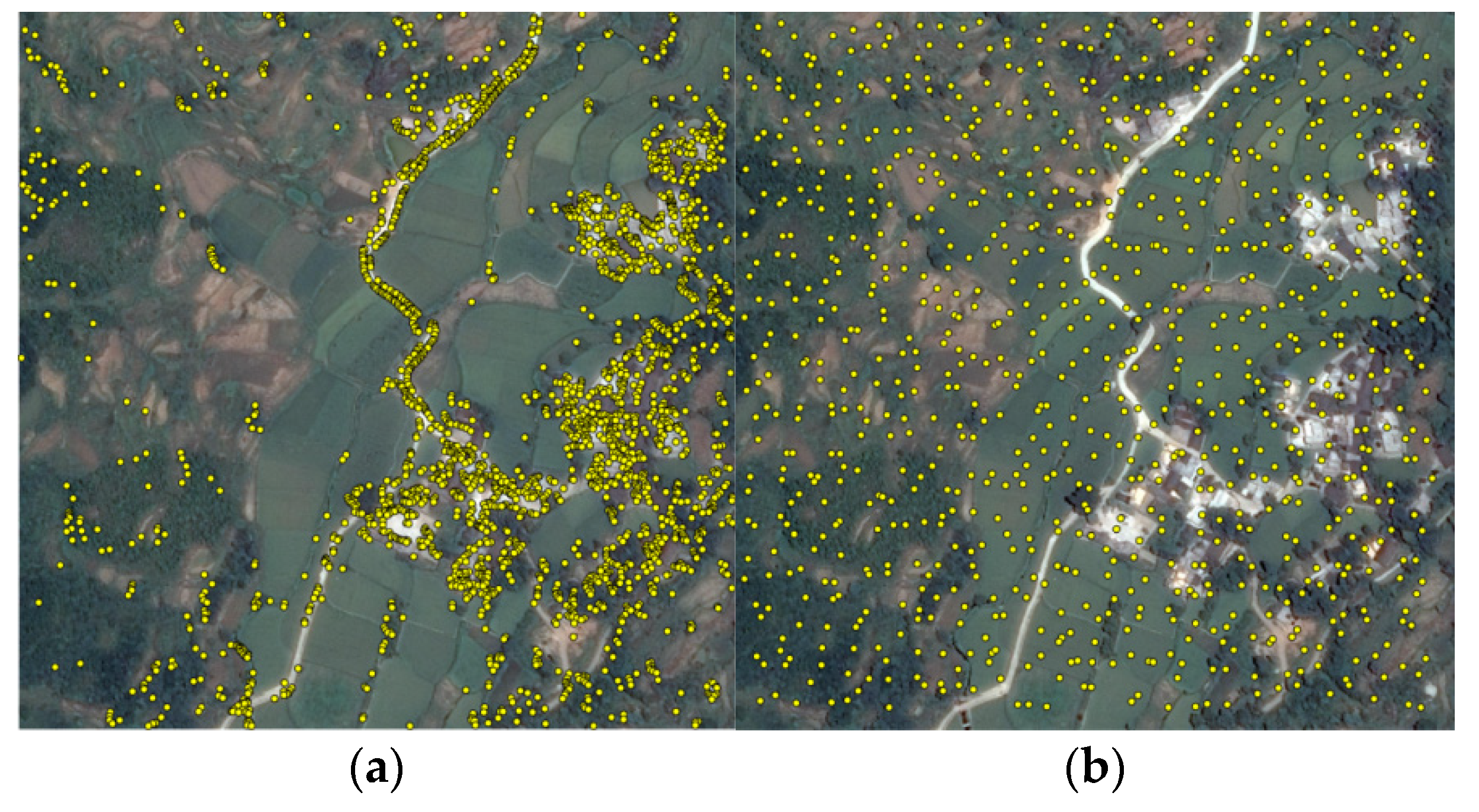
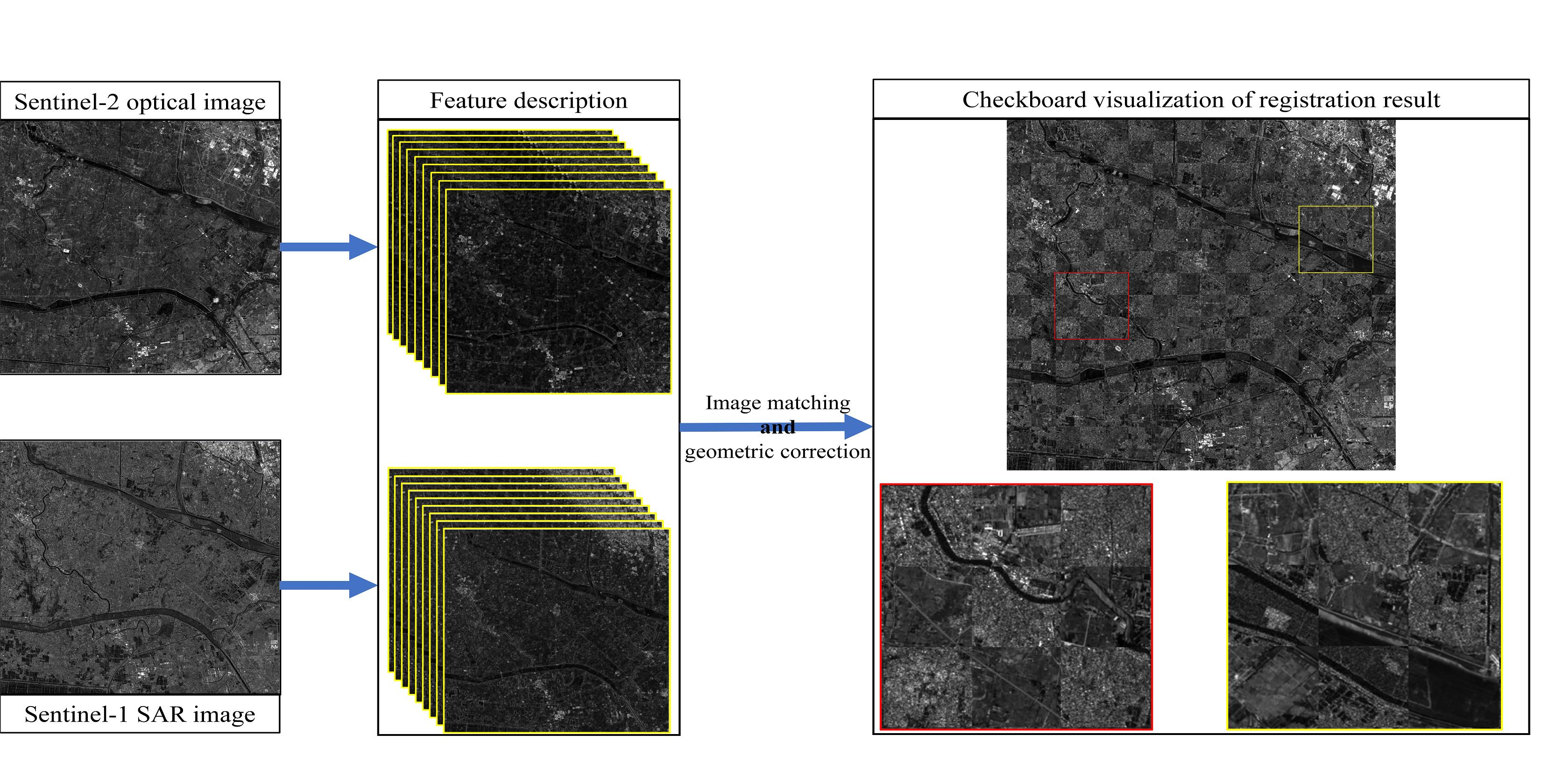
- We design a block-based matching scheme based on structural features to detect evenly distributed correspondences between the Sentinel-1 SAR L1 images and the Sentinel-2 optical L1C images, which is computationally effective and is robust to nonlinear radiometric differences.
- (2)
- We precisely measure the misregistration shifts between the Sentinel SAR and optical images.
- (3)
- We compare and analyze the registration accuracy of various geometric transformation models, and we determine an optimal model for the co-registration of the Sentinel SAR and optical images.
2. Sentinel-1 SAR and Sentinel-2 Optical Data Introduction
3. Methodology
3.1. Detection of Correspondences or CPs
3.1.1. Interest Point Detection
3.1.2. Structure Feature Extraction
3.1.3. Interest Point Matching
3.1.4. Mismatch Elimination
3.2. Mathematical Models of Geometric Transformation
3.2.1. Polynomial Models
3.2.2. Projective Models
3.2.3. RFM
3.3. Image Co-Registration
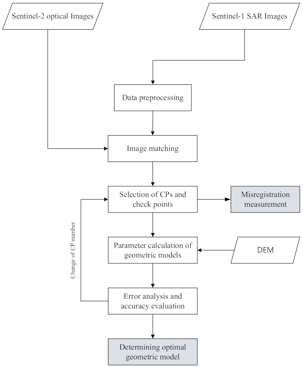
3.3.1. Data Preprocessing
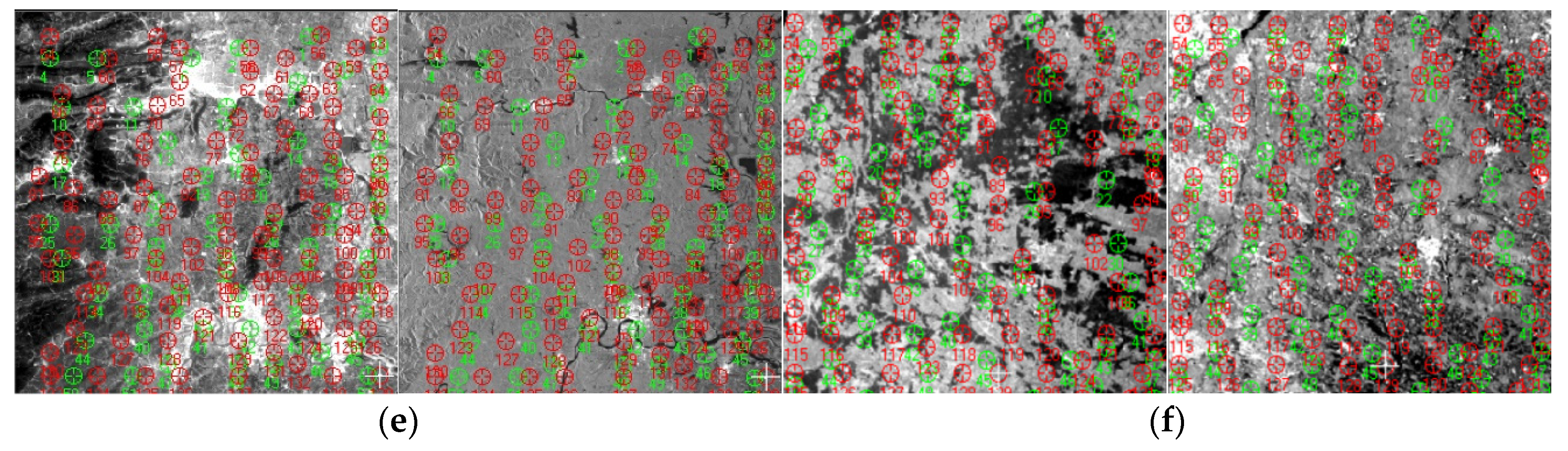
3.3.2. Image Matching
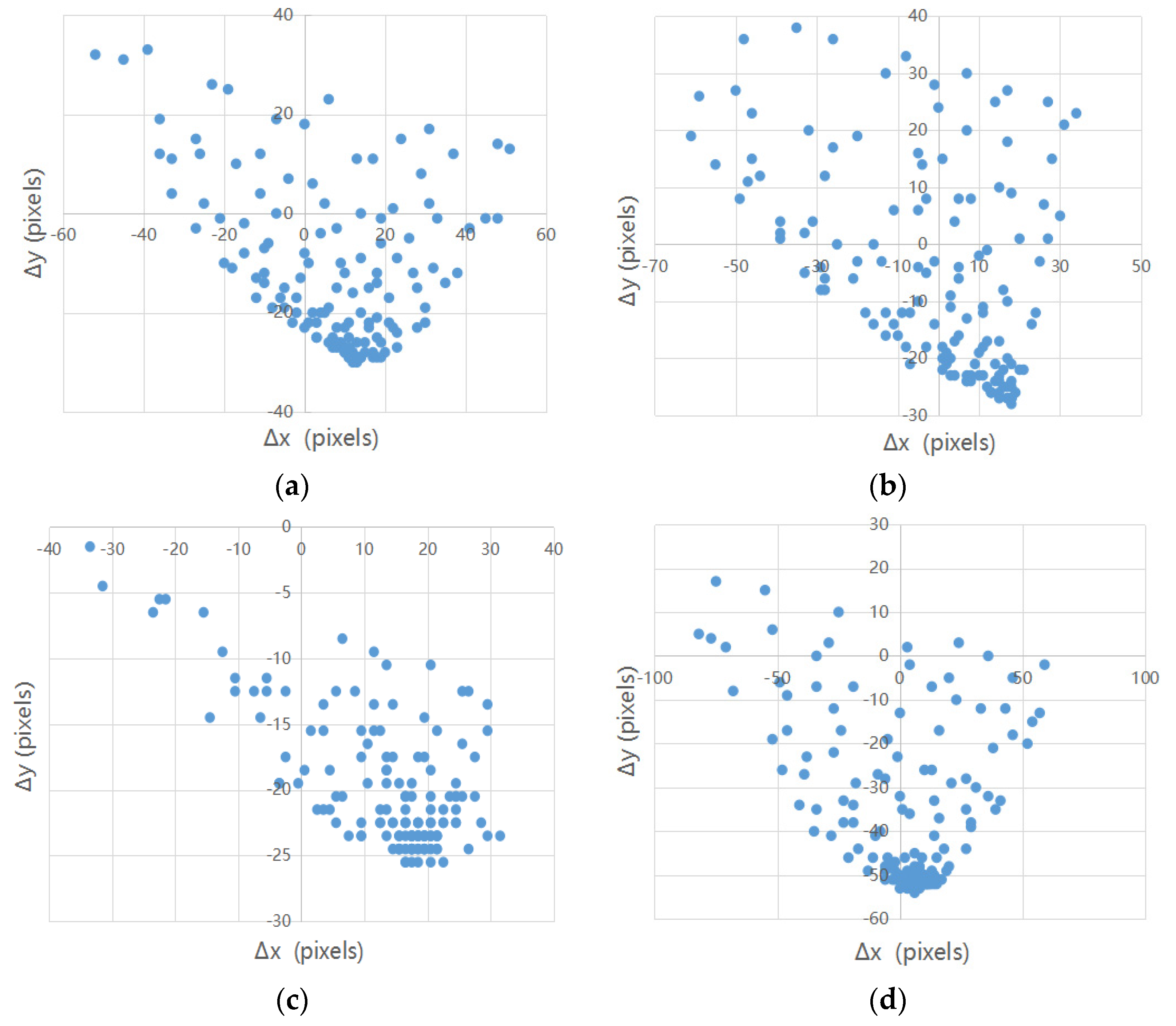
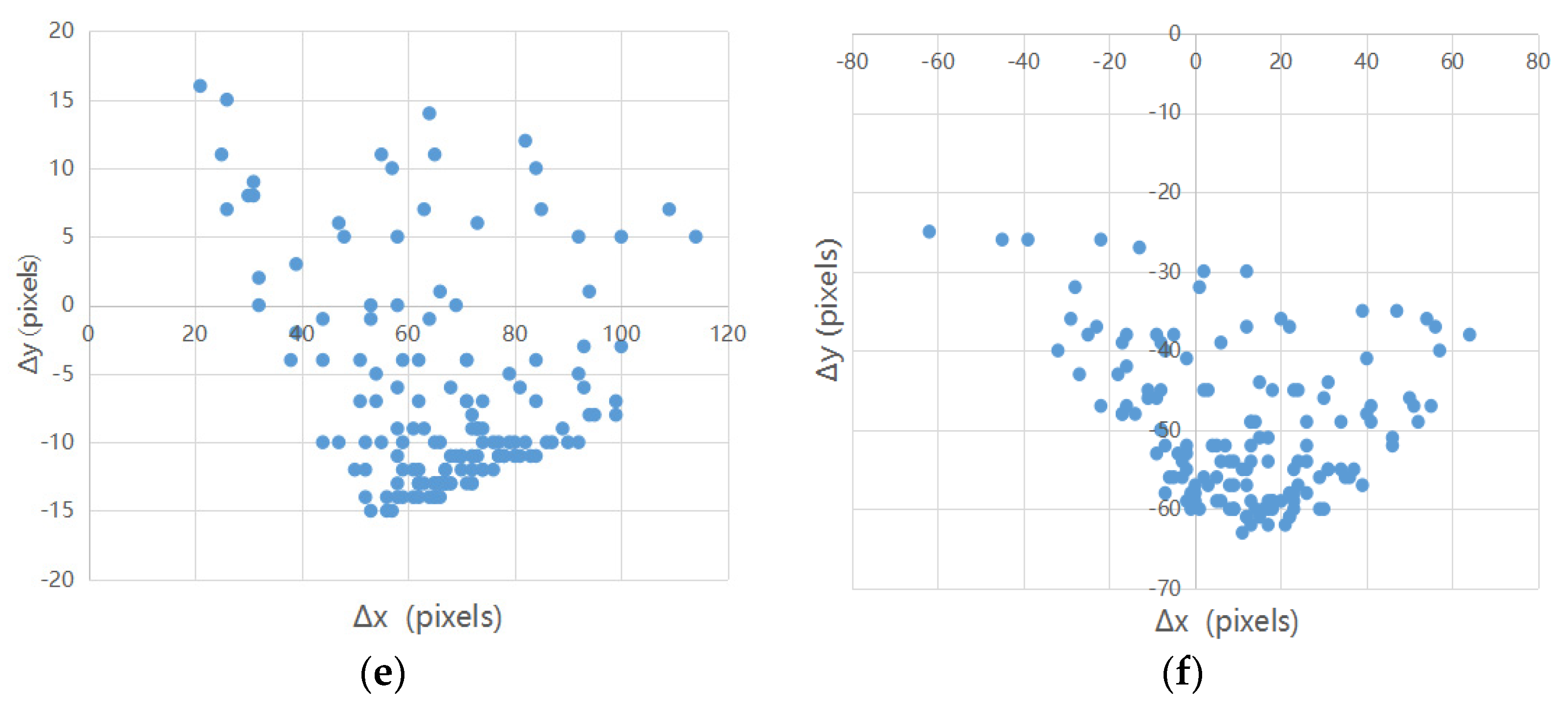
3.3.3. Misregistration Measurement
3.3.4. Parameter Calculation of Geometric Models
3.3.5. Accuracy Analysis and Evolution
4. Experiments
4.1. Experimental Data
4.2. Image Matching
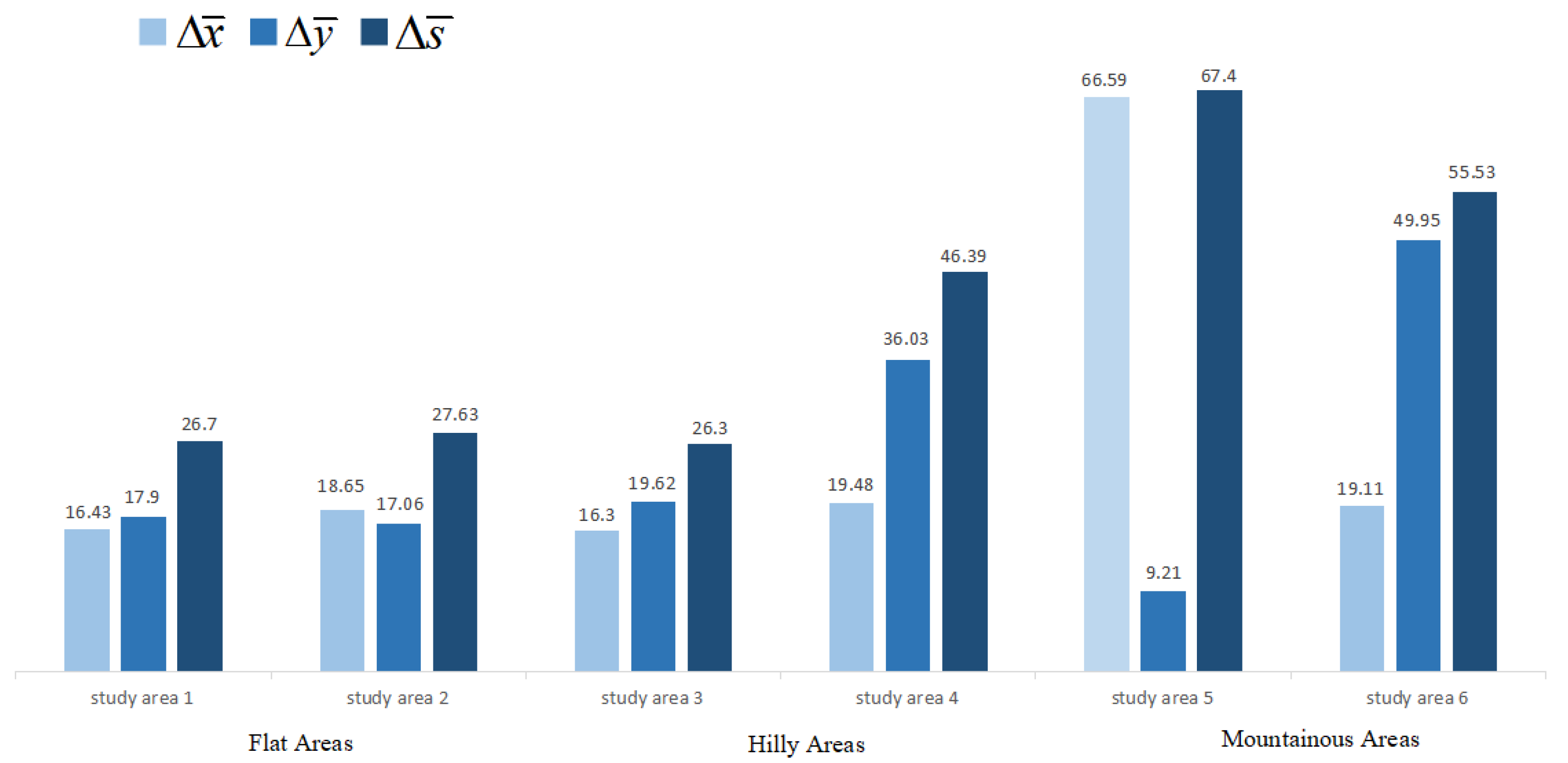
4.3. Misregistration Measurement
4.4. Co-Registration Accuracy Analysis and Evaluation
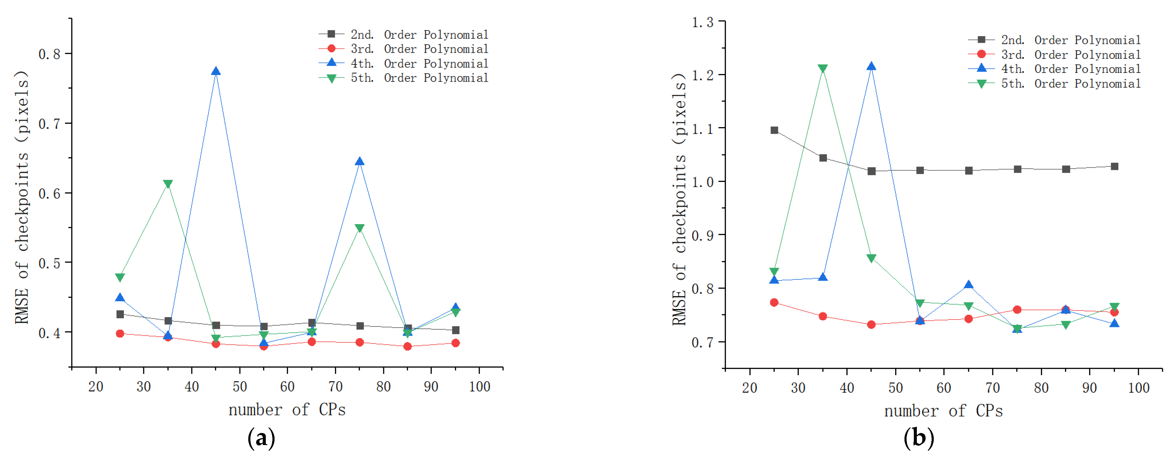
4.4.1. Accuracy Analysis of Flat Areas
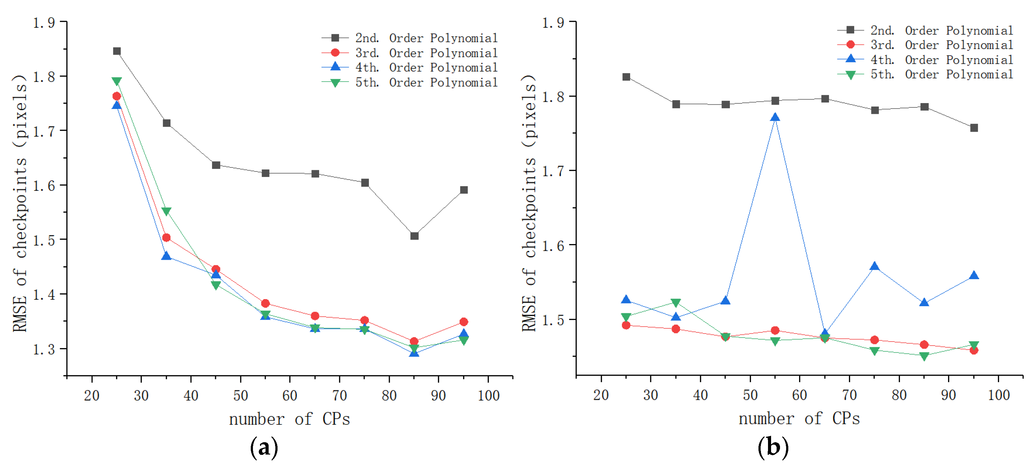
4.4.2. Accuracy Analysis of Hilly Areas
4.4.3. Accuracy Analysis of Mountainous Areas
4.4.4. Evaluation of Registration Results
5. Discussion and Conclusions
Author Contributions
Funding
Institutional Review Board Statement
Informed Consent Statement
Data Availability Statement
Conflicts of Interest
References
- Scarpa, G.; Gargiulo, M.; Mazza, A.; Gaetano, R. A CNN-Based Fusion Method for Feature Extraction from Sentinel Data. Remote Sens. 2018, 10, 236. [Google Scholar] [CrossRef] [Green Version]
- Haas, J.; Ban, Y. Sentinel-1A SAR and sentinel-2A MSI data fusion for urban ecosystem service mapping. Remote Sens. Appl. Soc. Environ. 2017, 8, 41–53. [Google Scholar] [CrossRef]
- He, W.; Yokoya, N. Multi-Temporal Sentinel-1 and -2 Data Fusion for Optical Image Simulation. ISPRS Int. J. Geo Inf. 2018, 7, 389. [Google Scholar] [CrossRef] [Green Version]
- Meraner, A.; Ebel, P.; Zhu, X.X.; Schmitt, M. Cloud removal in Sentinel-2 imagery using a deep residual neural network and SAR-optical data fusion. ISPRS J. Photogramm. Remote Sens. 2020, 166, 333–346. [Google Scholar] [CrossRef]
- Urban, M.; Berger, C.; Mudau, T.; Heckel, K.; Truckenbrodt, J.; Onyango Odipo, V.; Smit, I.; Schmullius, C. Surface Moisture and Vegetation Cover Analysis for Drought Monitoring in the Southern Kruger National Park Using Sentinel-1, Sentinel-2, and Landsat-8. Remote Sens. 2018, 10, 1482. [Google Scholar] [CrossRef] [Green Version]
- Chang, J.; Shoshany, M. Mediterranean shrublands biomass estimation using Sentinel-1 and Sentinel-2. In Proceedings of the 2016 IEEE International Geoscience and Remote Sensing Symposium (IGARSS), Beijing, China, 10–15 June 2016; pp. 5300–5303. [Google Scholar]
- Clerici, N.; Valbuena Calderón, C.A.; Posada, J.M. Fusion of Sentinel-1A and Sentinel-2A data for land cover mapping: A case study in the lower Magdalena region, Colombia. J. Maps 2017, 13, 718–726. [Google Scholar] [CrossRef] [Green Version]
- Whyte, A.; Ferentinos, K.P.; Petropoulos, G.P. A new synergistic approach for monitoring wetlands using Sentinels -1 and 2 data with object-based machine learning algorithms. Environ. Model. Softw. 2018, 104, 40–54. [Google Scholar] [CrossRef] [Green Version]
- Ye, Y.; Shan, J. A local descriptor based registration method for multispectral remote sensing images with non-linear intensity differences. ISPRS J. Photogramm. Remote Sens. 2014, 90, 83–95. [Google Scholar] [CrossRef]
- Zitová, B.; Flusser, J. Image registration methods: A survey. Image Vis. Comput. 2003, 21, 977–1000. [Google Scholar] [CrossRef] [Green Version]
- Harris, C.; Stephens, M. A Combined Edge and Corner Detector. In Proceedings of the fourth Alvey Vision Conference (ACV88), Manchester, UK, September 1988; pp. 147–152. [Google Scholar]
- Lowe, D.G. Distinctive Image Features from Scale-Invariant Keypoints. Int. J. Comput. Vis. 2004, 60, 91–110. [Google Scholar] [CrossRef]
- Bay, H.; Ess, A.; Tuytelaars, T.; Van Gool, L. Speeded-Up Robust Features (SURF). Comput. Vis. Image Underst. 2008, 110, 346–359. [Google Scholar] [CrossRef]
- Sedaghat, A.; Ebadi, H. Remote Sensing Image Matching Based on Adaptive Binning SIFT Descriptor. IEEE Trans. Geosci. Remote Sens. 2015, 53, 5283–5293. [Google Scholar] [CrossRef]
- Bouchiha, R.; Besbes, K. Automatic Remote-sensing Image Registration Using SURF. Int. J. Comput. Theory Eng. 2013, 5, 88–92. [Google Scholar] [CrossRef] [Green Version]
- Fan, J.; Wu, Y.; Li, M.; Liang, W.; Cao, Y. SAR and Optical Image Registration Using Nonlinear Diffusion and Phase Congruency Structural Descriptor. IEEE Trans. Geosci. Remote Sens. 2018, 56, 5368–5379. [Google Scholar] [CrossRef]
- Hel-Or, Y.; Hel-Or, H.; David, E. Matching by Tone Mapping: Photometric Invariant Template Matching. IEEE Trans. Pattern Anal. Mach. Intell. 2014, 36, 317–330. [Google Scholar] [CrossRef]
- Suri, S.; Reinartz, P. Mutual-Information-Based Registration of TerraSAR-X and Ikonos Imagery in Urban Areas. IEEE Trans. Geosci. Remote Sens. 2010, 48, 939–949. [Google Scholar] [CrossRef]
- Dalal, N.; Triggs, B. Histograms of Oriented Gradients for Human Detection. In Proceedings of the 2005 IEEE Computer Society Conference on Computer Vision and Pattern Recognition (CVPR’05), San Diego, CA, USA, 20–25 June 2005; pp. 886–893. [Google Scholar]
- Shechtman, E.; Irani, M. Matching Local Self-Similarities across Images and Videos. In Proceedings of the 2007 IEEE Conference on Computer Vision and Pattern Recognition, Minneapolis, MN, USA, 17–27 June 2007; pp. 1–8. [Google Scholar]
- Ye, Y.; Shan, J.; Bruzzone, L.; Shen, L. Robust Registration of Multimodal Remote Sensing Images Based on Structural Similarity. IEEE Trans. Geosci. Remote Sens. 2017, 55, 2941–2958. [Google Scholar] [CrossRef]
- Yan, X.; Zhang, Y.; Zhang, D.; Hou, N. Multimodal image registration using histogram of oriented gradient distance and data-driven grey wolf optimizer. Neurocomputing 2020, 392, 108–120. [Google Scholar] [CrossRef]
- Ye, Y.; Shen, L.; Hao, M.; Wang, J.; Xu, Z. Robust Optical-to-SAR Image Matching Based on Shape Properties. IEEE Geosci. Remote Sens. Lett. 2017, 14, 564–568. [Google Scholar] [CrossRef]
- Ye, Y.; Bruzzone, L.; Shan, J.; Bovolo, F.; Zhu, Q. Fast and Robust Matching for Multimodal Remote Sensing Image Registration. IEEE Trans. Geosci. Remote Sens. 2019, 57, 9059–9070. [Google Scholar] [CrossRef] [Green Version]
- El-Manadili, Y.; Novak, K. Precision rectification of SPOT imagery using the Direct Linear Transformation model. Photogramm. Eng. Remote Sens. 1996, 62, 67–72. [Google Scholar]
- Okamoto, A. An alternative approach to the triangulation of spot imagery. Int. Arch. Photogramm. Remote Sens. 1998, 32, 457–462. [Google Scholar]
- Smith, D.P.; Atkinson, S.F. Accuracy of rectification using topographic map versus GPS ground control points. Photogramm. Eng. Remote Sens. 2001, 67, 565–570. [Google Scholar]
- Gao, J. Non-differential GPS as an alternative source of planimetric control for rectifying satellite imagery. Photogramm. Eng. Remote Sens. 2001, 67, 49–55. [Google Scholar]
- Shaker, A.; Shi, W.; Barakat, H. Assessment of the rectification accuracy of IKONOS imagery based on two-dimensional models. Int. J. Remote Sens. 2005, 26, 719–731. [Google Scholar] [CrossRef]
- Dowman, L.; Dolloff, J.T. An evaluation of relational functions for photogrammetric restitution. Int. Arch. Photogramm. Remote Sens. 2000, 33, 254–266. [Google Scholar]
- Tao, C.V.; Hu, Y. A comprehensive study of the rational function model for photogrammetric processing. Photogramm. Eng. Remote Sens. 2001, 67, 1347–1357. [Google Scholar]
- Tao, C.V.; Hu, Y. 3D reconstruction methods based on the rational function model. Photogramm. Eng. Remote Sens. 2002, 68, 705–714. [Google Scholar]
- Hu, Y.; Tao, C.V. Updating solutions of the rational function model using additional control information. Photogramm. Eng. Remote Sens. 2002, 68, 715–723. [Google Scholar]
- Fraser, C.; Baltsavias, E.; Gruen, A. Processing of Ikonos imagery for submetre 3D positioning and building extraction. ISPRS J. Photogramm. Remote Sens. 2002, 56, 177–194. [Google Scholar]
- Fraser, C.; Hanley, H.; Yamakawa, T. Three-Dimensional Geopositioning Accuracy of Ikonos Imagery. Photogramm. Rec. 2002, 17, 465–479. [Google Scholar] [CrossRef]
- Schubert, A.; Small, D.; Miranda, N.; Geudtner, D.; Meier, E. Sentinel-1A Product Geolocation Accuracy: Commissioning Phase Results. Remote Sens. 2015, 7, 9431–9449. [Google Scholar] [CrossRef] [Green Version]
- Languille, F.; Déchoz, C.; Gaudel, A.; Greslou, D.; de Lussy, F.; Trémas, T.; Poulain, V. Sentinel-2 geometric image quality commissioning: First results. In Proceedings of the Image and Signal Processing for Remote Sensing XXI, Toulouse, France, 21–23 September 2015; p. 964306. [Google Scholar]
- Schubert, A.; Miranda, N.; Geudtner, D.; Small, D. Sentinel-1A/B Combined Product Geolocation Accuracy. Remote Sens. 2017, 9, 607. [Google Scholar] [CrossRef] [Green Version]
- Schmidt, K.; Reimann, J.; Ramon, N.T.; Schwerdt, M. Geometric Accuracy of Sentinel-1A and 1B Derived from SAR Raw Data with GPS Surveyed Corner Reflector Positions. Remote Sens. 2018, 10, 523. [Google Scholar] [CrossRef] [Green Version]
- Yan, L.; Roy, D.P.; Li, Z.; Zhang, H.K.; Huang, H. Sentinel-2A multi-temporal misregistration characterization and an orbit-based sub-pixel registration methodology. Remote Sens. Environ. 2018, 215, 495–506. [Google Scholar] [CrossRef]
- Barazzetti, L.; Cuca, B.; Previtali, M. Evaluation of registration accuracy between Sentinel-2 and Landsat 8. In Proceedings of the Fourth International Conference on Remote Sensing and Geoinformation of the Environment (RSCy2016), Paphos, Cyprus, 4–8 April 2016; p. 968809. [Google Scholar]
- Yan, L.; Roy, D.; Zhang, H.; Li, J.; Huang, H. An Automated Approach for Sub-Pixel Registration of Landsat-8 Operational Land Imager (OLI) and Sentinel-2 Multi Spectral Instrument (MSI) Imagery. Remote Sens. 2016, 8, 520. [Google Scholar] [CrossRef] [Green Version]
- Skakun, S.; Roger, J.-C.; Vermote, E.F.; Masek, J.G.; Justice, C.O. Automatic sub-pixel co-registration of Landsat-8 Operational Land Imager and Sentinel-2A Multi-Spectral Instrument images using phase correlation and machine learning based mapping. Int. J. Digit. Earth 2017, 10, 1253–1269. [Google Scholar] [CrossRef] [PubMed]
- Stumpf, A.; Michéa, D.; Malet, J.-P. Improved Co-Registration of Sentinel-2 and Landsat-8 Imagery for Earth Surface Motion Measurements. Remote Sens. 2018, 10, 160. [Google Scholar] [CrossRef] [Green Version]
- ESA. Sentinel-2 ESA’s optical high-resolution mission for GMES operational services (ESA SP-1322/). 2012. Available online: http://esamultimedia.esa.int/multimedia/publications/SP-1322_2/offline/download.pdf. (accessed on 10 February 2021).
- ESA. Sentinel-1 Product Definition. Ref: S1-RS-MDA-52-7440, Issue: 02, Date: 25/03/2016. 2016. Available online: https://sentinel.esa.int/documents/247904/1877131/Sentinel-1-Product-Definition (accessed on 10 February 2021).
- Sentinel-SAR User Guides. Available online: https://sentinels.copernicus.eu/web/sentinel/user-guides/sentinel-1-sar/product-types-processing-levels/level-1 (accessed on 10 February 2021).
- Xiang, Y.; Tao, R.; Wan, L.; Wang, F.; You, H. OS-PC: Combining Feature Representation and 3-D Phase Correlation for Subpixel Optical and SAR Image Registration. IEEE Trans. Geosci. Remote Sens. 2020, 58, 6451–6466. [Google Scholar] [CrossRef]
- Moravec, H. Obstacle Avoidance and Navigation in the Real World by a Seeing Robot Rover. Doctoral Dissertation, Stanford University, Stanford, CA, USA, 1980; pp. 1–92. [Google Scholar]
- Rosten, E.; Drummond, T. Machine Learning for High-Speed Corner Detection. In Proceedings of the 9th European Conference on Computer Vision, Part I, Graz, Austria, 7–13 May 2006; pp. 430–443. [Google Scholar]
- Fischler, M.A.; Bolles, R.C. Random sample consensus: A paradigm for model fitting with applications to image analysis and automated cartography. Commun. ACM 1981, 24, 381–395. [Google Scholar] [CrossRef]


| Order of Polynomials | Cases | Number of Parameters | Min. Number of CPs |
| 1 | P2 = P4 = 1 P2 = P4 P2 ≠ P4 | 8 11 14 | 4 6 7 |
| 2 | P2 = P4 = 1 P2 = P4 P2 ≠ P4 | 20 29 38 | 10 15 19 |
| 3 | P2 = P4 = 1 P2 = P4 P2 ≠ P4 | 40 59 78 | 20 30 39 |
| Area Type | No. | Lat/Lon Range | SAR | Optical | Image Characteristic |
| Date Size (pixels) | Date Size (pixels) | ||||
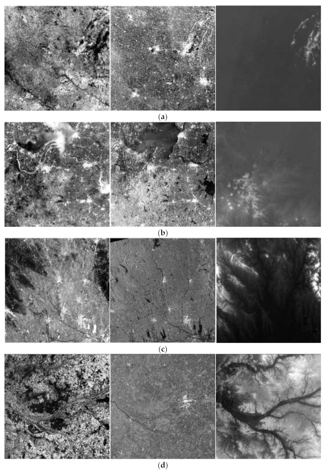
| Flat | Study 1 | 33.35° N 34.34° N 115.91° E 117.11° E | 06 August 2018 10,980 × 10,980 | 12 October 2018 10,980 × 10,980 | Images located in the midwest of the North China Plain. From the DEM map in Figure 5a, most of the area is at elevations below 50 m except for few highlands in the upper right corner of the area reaching an elevation of about 130 m. The maximum elevation difference is less than 120 m; therefore, the area is classified as a flat terrain. |
| Study 2 | 32.43° N 33.43° N 118.06° E 119.26° E | 04 April 2018 10,980 × 10,980 | 28 March 2018 10,980 × 10,980 | Images located in the plain at the junction of Anhui and Jiangsu provinces, China. The terrain fluctuation is small and the elevation is below 160 m. From the DEM map in Figure 5b, although there are some small hills in the southwest corner of the area, more than 75% of the area is flat and the maximum elevation difference is about 150 m. Therefore, the area is classified as a flat terrain. | |
| Hill | Study 3 | 30.60° N 31.62° N 113.09° E 114.26° E | 19 April 2018 10,980 × 10,980 | 18 April 2018 10,980 × 10,980 | Images located in the northeast of Hubei province, China. From the DEM map in Figure 5c, the northwest and northeast of the area are surrounded by many hills. The overall elevation range is between 10 m and 250 m, and the elevation of two-thirds of the area is below 100 m. The maximum elevation difference is about 200 m; therefore, the area is classified as a hilly terrain. |
| Study 4 | 46.79° N 47.82° N 0.38° W 1.14° E | 12 August 2018 10,980 × 10,980 | 02 August 2018 10,980 × 10,980 | Images located in the midwest of France, centered at Tours city. From the DEM map in Figure 5d, the area has many hills and presents an undulating terrain. The maximum elevation difference reaches 200 m; therefore, the area is classified as a hilly terrain. | |
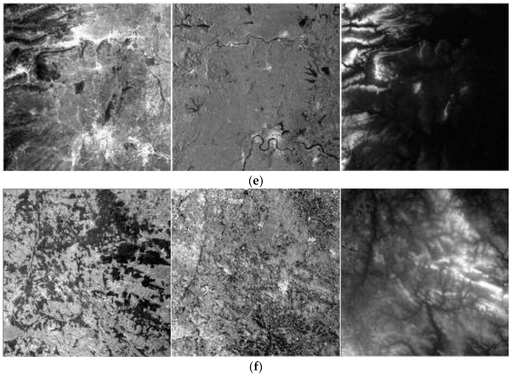
| Mountain | Study 5 | 28.83° N 29.83° N 110.99° E 112.14° E | 27 September 2018 10,980 × 10,980 | 05 October 2018 10,980 × 10,980 | Images located in the western area of Changde City, Hunan Province, China. From the DEM map in Figure 5e, there is a great contrast in elevation between the east and west of the area. The west is covered by mountains and the elevation is about 700–800 m, while the east is an urban area with elevation ranging from 10 m to 150 m. The overall terrain undulates greatly, with a maximum elevation difference of nearly 800 m. Therefore, the area is classified as a mountainous terrain. |
| Study 6 | 50.46° N 51.45° N 19.56° E 21.14° E | 24 February 2018 10,980 × 10,980 | 24 February 2019 10,980 × 10,980 | Images located in southeastern Poland, with Kielce city as the center. From the DEM map in Figure 5f, the mountain range crosses the image area diagonally. Although there are no obvious peaks, the elevation distribution is very complex, floating around 190–500 m, with a maximum elevation difference of 300 m; therefore, the area is classified as a mountainous terrain. |
| No. | Number of Extracted Interest Points | Number of Correspondences | Time (s) | Scene Type |
| Study 1 | 400 | 318 | 6.59 | Flat area |
| Study 2 | 400 | 259 | 6.52 | Flat area |
| Study 3 | 400 | 304 | 6.57 | Hilly area |
| Study 4 | 400 | 172 | 6.65 | Hilly area |
| Study 5 | 400 | 275 | 6.62 | Mountainous area |
| Study 6 | 400 | 186 | 6.67 | Mountainous area |
| Area Type | No. | Maximal | Minimal | STD | |||
| Flat | Study 1 | 16.43 | 17.90 | 26.70 | 61.06 | 5.39 | 9.84 |
| Study 2 | 18.65 | 17.06 | 27.63 | 91.24 | 31.62 | 11.79 | |
| Hill | Study 3 | 16.30 | 19.62 | 26.30 | 39.30 | 10.70 | 6.05 |
| Study 4 | 19.48 | 36.03 | 46.39 | 82.15 | 3.61 | 12.06 | |
| Mountain | Study 5 | 66.59 | 9.21 | 67.40 | 114.11 | 26.40 | 16.80 |
| Study 6 | 19.11 | 49.95 | 55.53 | 74.43 | 29.97 | 9.13 |
| Geometric Model | Study Area 1 | Study Area 2 | ||
|---|---|---|---|---|
| Maximum Residual | RMSE | Maximum Residual | RMSE | |
| 1st-order polynomial | 28.90 | 10.29 | 33.74 | 11.78 |
| 2nd-order polynomial | 0.78 | 0.40 | 3.42 | 1.03 |
| 3rd-order polynomial | 0.75 | 0.38 | 3.45 | 0.76 |
| 4th-order polynomial | 0.92 | 0.44 | 2.98 | 0.74 |
| 5th-order polynomial | 0.68 | 0.43 | 3.63 | 0.77 |
| 10-parameter projective transformation | 10.19 | 4.38 | 10.11 | 4.53 |
| 22-parameter projective transformation | 1.29 | 0.60 | 3.07 | 1.16 |
| 38-parameter projective transformation | 1.51 | 0.70 | 4.47 | 1.43 |
| 1st-order RFM (same denominator) | 24.46 | 8.31 | 21.79 | 7.11 |
| 1st-order RFM (different denominator) | 9.73 | 4.38 | 9.18 | 4.41 |
| 2nd-order RFM (same denominator) | 7.68 | 1.42 | 11.45 | 3.50 |
| 2nd-order RFM (different denominator) | 1.94 | 0.68 | 4.67 | 1.46 |
| 3rd-order RFM (same denominator) | 6.02 | 1.28 | 13.34 | 3.27 |
| 3rd-order RFM (different denominator) | 1.03 | 0.70 | 3.77 | 1.27 |
| Geometric Model | Study Area 3 | Study Area 4 | ||
|---|---|---|---|---|
| Maximum Residual | RMSE | Maximum Residual | RMSE | |
| 1st-order polynomial | 29.71 | 12.17 | 32.03 | 12.95 |
| 2nd-order polynomial | 4.76 | 1.59 | 6.34 | 1.76 |
| 3rd-order polynomial | 4.07 | 1.35 | 3.27 | 1.46 |
| 4th-order polynomial | 3.74 | 1.33 | 3.32 | 1.56 |
| 5th-order polynomial | 3.91 | 1.32 | 3.39 | 1.47 |
| 10-parameter projective transformation | 10.76 | 4.02 | 9.92 | 5.45 |
| 22-parameter projective transformation | 5.79 | 2.11 | 5.28 | 2.47 |
| 38-parameter projective transformation | 4.43 | 1.83 | 6.65 | 2.39 |
| 1st-order RFM (same denominator) | 24.72 | 7.43 | 25.33 | 8.59 |
| 1st-order RFM (different denominator) | 8.03 | 3.37 | 11.43 | 5.20 |
| 2nd-order RFM (same denominator) | 14.24 | 3.82 | 13.12 | 4.86 |
| 2nd-order RFM (different denominator) | 5.53 | 1.84 | 6.67 | 2.34 |
| 3rd-order RFM (same denominator) | 8.87 | 2.90 | 8.85 | 4.33 |
| 3rd-order RFM (different denominator) | 4.80 | 1.64 | 5.46 | 1.86 |
| Geometric Model | Study Area 5 | Study Area 6 | ||
|---|---|---|---|---|
| Maximum Residual | RMSE | Maximum Residual | RMSE | |
| 1st-order polynomial | 35.55 | 14.41 | 48.58 | 17.94 |
| 2nd-order polynomial | 5.13 | 2.77 | 13.48 | 3.63 |
| 3rd-order polynomial | 4.14 | 1.74 | 5.76 | 2.29 |
| 4th-order polynomial | 4.48 | 1.70 | 5.82 | 2.31 |
| 5th-order polynomial | 4.33 | 1.65 | 8.32 | 2.83 |
| 10-parameter projective transformation | 9.98 | 3.43 | 17.47 | 8.48 |
| 22-parameter projective transformation | 7.31 | 2.03 | 7.03 | 3.48 |
| 38-parameter projective transformation | 5.11 | 1.80 | 8.53 | 3.37 |
| 1st-order RFM (same denominator) | 20.98 | 6.57 | 45.31 | 14.95 |
| 1st-order RFM (different denominator) | 10.26 | 2.95 | 18.17 | 7.59 |
| 2nd-order RFM (same denominator) | 5.11 | 2.08 | 15.67 | 8.01 |
| 2nd-order RFM (different denominator) | 4.16 | 1.82 | 7.82 | 3.25 |
| 3rd-order RFM (same denominator) | 5.94 | 2.14 | 14.30 | 6.68 |
| 3rd-order RFM (different denominator) | 4.38 | 1.84 | 4.33 | 2.44 |
| No. | Proposed Method | Terrain Correction | Scene Type | ||
|---|---|---|---|---|---|
| RMSE (pixels) | Time (s) | RMSE (pixels) | Time (s) | ||
| Study 1 | 0.38 | 9.59 | 0. 92 | 909 | Flat area |
| Study 2 | 0.76 | 9.52 | 1.12 | 892 | Flat area |
| Study 3 | 1.35 | 9.57 | 1.52 | 917 | Hilly area |
| Study 4 | 1.46 | 9.65 | 1.61 | 904 | Hilly area |
| Study 5 | 1.74 | 9.62 | 1.87 | 898 | Mountainous area |
| Study 6 | 2.29 | 9.67 | 2.27 | 919 | Mountainous area |
Publisher’s Note: MDPI stays neutral with regard to jurisdictional claims in published maps and institutional affiliations. |
© 2021 by the authors. Licensee MDPI, Basel, Switzerland. This article is an open access article distributed under the terms and conditions of the Creative Commons Attribution (CC BY) license (http://creativecommons.org/licenses/by/4.0/).
Share and Cite
Ye, Y.; Yang, C.; Zhu, B.; Zhou, L.; He, Y.; Jia, H. Improving Co-Registration for Sentinel-1 SAR and Sentinel-2 Optical Images. Remote Sens. 2021, 13, 928. https://doi.org/10.3390/rs13050928
Ye Y, Yang C, Zhu B, Zhou L, He Y, Jia H. Improving Co-Registration for Sentinel-1 SAR and Sentinel-2 Optical Images. Remote Sensing. 2021; 13(5):928. https://doi.org/10.3390/rs13050928
Chicago/Turabian StyleYe, Yuanxin, Chao Yang, Bai Zhu, Liang Zhou, Youquan He, and Huarong Jia. 2021. "Improving Co-Registration for Sentinel-1 SAR and Sentinel-2 Optical Images" Remote Sensing 13, no. 5: 928. https://doi.org/10.3390/rs13050928