Abstract
CORINE Land-Cover (CLC) and its by-products are considered as a reference baseline for land-cover mapping over Europe and subsequent applications. CLC is currently tediously produced each six years from both the visual interpretation and the automatic analysis of a large amount of remote sensing images. Observing that various European countries regularly produce in parallel their own land-cover country-scaled maps with their own specifications, we propose to directly infer CORINE Land-Cover from an existing map, therefore steadily decreasing the updating time-frame. No additional remote sensing image is required. In this paper, we focus more specifically on translating a country-scale remote sensed map, OSO (France), into CORINE Land Cover, in a supervised way. OSO and CLC not only differ in nomenclature but also in spatial resolution. We jointly harmonize both dimensions using a contextual and asymmetrical Convolution Neural Network with positional encoding. We show for various use cases that our method achieves a superior performance than the traditional semantic-based translation approach, achieving an 81% accuracy over all of France, close to the targeted 85% accuracy of CLC.
1. Introduction
Over the last 30 years, land-cover maps became a mandatory baseline for monitoring the status and the dynamics of the Earth’s surface. For that purpose, despite being a notoriously time-consuming procedure, a large number of land-cover products has been generated covering the entire Earth surface multiple times [1,2], at several spatial scales, and with multiple representations (sets of classes, organized into what we call nomenclatures). Surprisingly, none of the existing maps fit to all specific end-users that continuously require products with higher spatial, semantic, and temporal resolutions [3]. However, moving back to the tedious traditional photo-interpretation task or revisiting the automatic analysis of large amounts of remotely sensed imagery using massive training/validation data sets should be avoided for complexity, time consumption and reproducibility issues [4]. One might prefer deriving new products from existing land-cover maps, assuming they are available on the desired spatial extent and with a representation close to the target one.
Such a strategy involves alleviating the discrepancies existing between maps in terms of spatial and semantic resolutions [5]. Such interleaved dissimilarities stem from the varying users’ requirements, rigid nomenclatures, technical constraints and solutions adopted for deriving the maps [6]: the remote sensing images used for the underlying supervised classification task, the amount and quality of training data and human intervention in all steps of the generation process [7,8], natively generate maps that are not identical nor straightforwardly comparable. All the above-mentioned requirements can be addressed through the pivotal development of land-cover translation solutions [9]. As an analogy with linguistics, we choose to call land-cover translation the process of generating a target land-cover map from a given (source) one. The source always exists whereas the target can either be virtual or real. In the former case, we aim to generate a new map based solely on the characteristics of the existing one. In the latter one, both maps already exist but we try to benefit from some advantages of the source map to improve the target one (temporally, spatially, or semantically). For maps being represented by classes, like any language translation task, the challenge lies in transforming a categorical representation into another one. In the land-cover field, translation, therefore, means modifying the nomenclature and the spatial scale (possibly jointly) of the source map in order to match the specifications of the target map. In the following, we exclude from the land-cover translation task cases where the target is virtual and where the source and target data are not spatially overlapping.
In this paper, we aim to produce a yearly updated country-scale version of the European land-cover reference database CORINE Land Cover (CLC), traditionally updated every 6 years. For that purpose, we propose a new supervised land-cover translation framework aiming to translate OSO, a France-wide yearly updated land-cover product, into CLC (Figure 1).
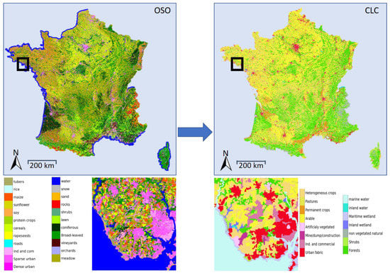
Figure 1.
Illustration of the land-cover translation task. The spatial and semantic transformation of a yearly map (OSO, left) into another (CLC, right) may lead to numerous applications such as fast updating or enhanced change detection.
In the literature, translation is an intermediate step. It is adopted either for map comparison or fusion purposes. In the first case, one aims to evaluate the quality of a map with respect to another one [10]. In the second one, the goal is to take the best of both representations [5,11] without a special focus on quality evaluation. This strategy is also named hybridization. In both contexts, this results in two main shortcomings: (i) a lack of formalization of the translation task, leading to the absence of versatile solutions, and (ii) no genuine quality assessment procedure. Indeed, translation errors are ignored in both cases. When fusing maps, individual errors are in practice balanced by stacking multiple products: only an agreement is targeted [7,12]. When comparing two maps, either a direct link between classes is performed or an intermediate representation is adopted (e.g., Land Cover Classification System, LCCS, [10]). Then, the same errors apply to both of them and are not taken into account. In the literature, the translation in terms of spatial resolution is usually overlooked using simple approaches such as the nearest neighbor resampling [13]. This ignores the challenge of nomenclature translation and may not preserve the realistic geographical boundaries and the shape of objects. Such solutions can achieve statistically acceptable results but fail in terms of cartographic quality. Generalization techniques may be relevant but are only adapted to process very few classes at the same time [14]. Most approaches for semantic translation rely on ad-hoc class correspondences between the two nomenclatures [15]. They assume that the geometry of the maps remains unchanged, that errors are limited or that discrepancies correspond to meaningful changes [1]. This prevents from adopting nomenclature translation for multiple use cases. Few works have tried to automatically match multiple representations. They concluded on the difficulty in dealing with category semantics [16].
Two main limitations of those commonly used strategies can be highlighted. First of all, spatial and semantic resolutions are highly intertwined, but never addressed jointly so far. Secondly, the traditional semantic-based method can be seen as analogous to a word-by-word translation of a sentence. Each class of the source nomenclature gets a translation into the target nomenclature in a spatial context-independent way, ignoring more complex semantic and spatial relationships. Consequently, current frameworks of land-cover translation drastically restrict the scope of what such a definition encompasses in reality. The core reason is that they are either too specific to a given problem or do not manage to correctly handle the interleaved issue of spatial and semantic shifts.
This paper makes the following contributions:
- A comprehensive analysis of the land-cover translation task with underlying challenges and potential methodological solutions.
- A novel framework, applied at a national scale, based on Convolutional Neural Networks that simultaneously and contextually translates semantic and spatial concepts from a state-of-the-art remote sensing based land-cover map (OSO, France) to an authoritative product, CORINE Land Cover. This framework paves the way for an annual update of CLC at country-scale.
- An application of our framework to three distinct use cases, in order to assess its performance under operational constraints and its relevance with respect to other conceivable solutions.
The remainder of this paper is organized as follows. In Section 2, we review the existing land-cover translation frameworks and associated main issues. In Section 3, we detail our OSO-to-CLC data set corresponding to the scenarios we investigate. Section 4 focuses on the proposed method and the proposed variations. Experiments and results are presented in Section 5. Finally, Section 6 presents some conclusions and outlooks.
2. Related Work
In this section, we discuss the existing methods that translate a land-cover representation to another one. We first describe the task according to the two main dimensions of the problem: the spatial resolution and the nomenclature. We then review existing solutions and their related issues when applied to the land-cover translation task. They encompass various operational challenges, depending on the source and the target maps, as depicted in Figure 2.
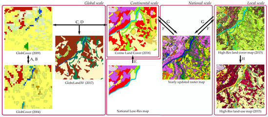
Figure 2.
Main possibilities for land-cover map translation. (A) change detection, (B) updating, (C) validation, (D) harmonization, (E) completion, (F) spatial simplification, (G) spatial improvement, (H) semantic modification. The method proposed in this paper can handle configurations (E,F,H). See text for more details. See [1] for more details about the existing land-cover maps.
2.1. Problem Description
As stated previously, land-cover translation involves two potential modifications, in terms of semantics and spatial resolution. We present below each of these aspects separately. However, one must notice that both are highly intertwined since the set of classes depends on the spatial resolution of the map and vice versa [3].
2.1.1. Semantic Translation:
The first modification consists of turning a source nomenclature into a target one. This step is necessary since nomenclatures are not standardized [5]. Even for spatially coincident maps, variations exist in terms of class due to political or technical choices. Indeed, there are two main reasons for the vast diversity of nomenclatures. The first one is that nomenclatures are defined for a specific context each time. The diversity of applications and end-users natively leads to either discrepant representations or representations at different levels of detail. The second reason is a technological one: a particular combination of data sources and processing methods constrains to discriminate a given set of classes that may significantly vary from a map to another.
Thus, many works have focused on finding an ideal nomenclature usable across all land-cover mapping projects [10,17]. However, no standardization technique is currently universally adopted due to their inherent constraints [18]. Translating one land-cover into another one needs a consistent link between the two nomenclatures. Two main approaches prevail (purely semantic or data-driven). They are described in Section 2.2. One way to recover such a link is to find semantic correspondences between the classes of the two nomenclatures. This kind of method is usually referred to as harmonization [15] (Figure 2D), which is pivotal for map updating, change detection, validation or hybridization (Figure 2A–C). Such task is often carried out manually. For instance, inspecting the definitions of the classes of two nomenclatures, one could infer that the class Dense urban in the source nomenclature perfectly fits the definition of the class Continuous urban in the target nomenclature. However, straightforward 1 → 1 or n → 1 correspondences are not always achievable when dealing with classes covering more complex concepts such as those related to land-use (Figure 2H). An alternative strategy consists of searching for correspondences in the data itself instead of the class definitions. In this case, two maps of the same area and the same period are compared through statistical analysis in order to derive the co-occurrence relationships mentioned above. More complex n → m behaviors can be captured.
2.1.2. Spatial Transformation:
It consists of modifying the spatial resolution of the map. The notion of spatial resolution encompasses two aspects: the theoretical minimum size (MS) for an object to be included in the map, and the minimum mapping unit (MMU), i.e., the effective minimum size. The first one is the same for all classes. It corresponds to the pixel size in raster format. The second one can vary across classes: specific classes can be preserved while not fitting to the initial specification such as linear classes (rivers, roads). Usually, when the map is produced by photo-interpretation of images, the MMU differs from the raster resolution while they usually are the same when the map is automatically produced from remote sensing data. The land-cover translation procedure needs to address both aspects.
When the source resolution is coarser than the target one, this is a super-resolution problem [19,20]. This allows addressing the mixed pixel problem (Figure 2G). Additional data, such as images, are often needed to retrieve the structural information [21]. When the source resolution is finer than the target one, a technique for source map simplification is needed. In remote sensing, the problem is well documented and is commonly known as down-sampling (Figure 2F): the interpolation of one value from multiple neighbors using an averaging technique can be used. In the case of categorical data, down-sampling is far more difficult. We have to deal with discrete values of which the order does not carry information: computing the average of two classes such as tree and water (e.g., with labels 2 and 15) does not make sense. The down-sampling task is assimilated in cartography to the generalization process [14]. Since all information can not be represented at a coarser scale, various transformations are performed in a hierarchical way to simplify, gather, remove, or modify individual elements of the source map [22]. Often, rules are manually defined to choose which information is kept, modified or erased, and subsequently only valid for two specific scales [23].
Land-cover maps usually include in their specifications an overall accuracy. A translation procedure has to be evaluated with respect to such a value. Reaching it may be difficult for at least two reasons. First, there are errors in the source map. With a standard accepted accuracy of about 85% [24], 15% of errors in the source map is to be expected. This can negatively impact any statistical translation method and can hardly be alleviated. In most products, the per-class and per-area accuracies are not provided except for very limited evaluation sets. They can be hardly learned. The second source of errors affecting the target accuracy is the map translation procedure itself. Ideally, a translation procedure should be error-free. Additionally, it could correct some systemic errors observed in the source data. For example, if confusion exists between two source classes, disambiguation is conceivable in the target domain, leading to more accurate discrimination than with simple nomenclature matching.
2.2. Literature Review
In this section, we review the existing techniques proposed to accomplish either semantic or spatial translation.
Traditional nomenclature harmonization techniques use purely semantic approaches [25] to establish a correspondence between two nomenclatures. The core idea is to define semantic relationships between each class of each nomenclature. Many methods have been proposed to find such 1 → 1 and 1 → n or n → 1 associations. A perfect translation is conceivable when one or more classes in the source nomenclature match with only one class in the target nomenclature (i.e., n → 1 relationship). Other cases are far more challenging and are poorly addressed by semantic methods [18,26,27]. Simple solutions rely on expert knowledge [28] and are hardly generalizable. When very specific classes are targeted, remote sensing data are often integrated to bring additional constraints [29]. More sophisticated solutions are based on semantic distances, computed on hierarchical nomenclature trees [30], semi-lattices [31] or class characteristics features [32]. The main advantage of a semantic distance based approach is that it defines a correspondence value between each source and target classes [33]. Unfortunately, when a source class has a small semantic distance with multiple target labels, the final translation will always result in the same target label (the closest of them all), ignoring all the other closely related labels that could have been more appropriate in a given context. Recent references in harmonization techniques include the well-known Land-Cover Classification System (LCCS) [34,35] and the EAGLE [36] framework, which try to overcome the rigidity of current solutions by defining pseudo embedding for each label and by matching them with the closest one. Their main limitation remains that they still only associate each source label with its closest one, despite the fact that they acknowledge the existence of other possible associations. Since semantic-based techniques usually exhibit such limitations, they are often combined with expert knowledge [37].
Another way of defining a relationship between nomenclatures is data-driven, with a direct comparison of pairs of maps. Statistical links between the nomenclatures are obtained by analyzing spatially co-occurring classes. For example, ref. [8] compared an expert-based association between nomenclatures with a confusion matrix computed between two maps. They reached a 57% agreement between both. This underlines the importance of improving current nomenclature translation techniques. A first naive approach inspired by the previous example would consist of using a confusion matrix between the source and the target maps and to assign to each source class the most likely class in the target nomenclature. Recently, Latent Dirichlet Allocation has been adopted in [2] as an unsupervised way to help with such a challenge. It exhibits two main limitations: it is not flexible and cannot handle correlated classes.
Note that these methods only rely on statistical association: they discard the spatial context and the geographical location of each object before translation. For example, the class grass of GlobeLand30 [38] can be translated into several CORINE Land Cover classes: Green urban areas, Sport and leisure facilities, Pastures, Natural grassland or Sparsely vegetated areas. In such cases, the analysis of the local neighborhood is required. This advocates for integrating the spatial context in the translation task. As in natural language processing (NLP), land-cover translation involves too many possible contextual configurations and cannot be manually defined. In NLP, this issue is tackled using machine learning procedures on text corpora [39]. Surprisingly, no attempt of land-cover translation using machine learning based contextual translation frameworks has been proposed in the literature so far.
Compared to semantic translation, spatial resolution transformation has been under-addressed in the land-cover mapping field. A vast majority of studies use a simple resampling strategy: a majority rule [40] or the nearest neighbor method [41]. They are adopted for the down-sampling case, while being sub-optimal. They are not adequate for the super-resolution task. The most natural yet unrealistic solution for spatial translation is to manually derive a set of rules based on the analysis of all possible spatial configurations in the context of an object. For down-sampling, this would imply defining a set of rules for summarizing information of the source map. However, it is combinatorially expensive even if we limit ourselves to coherent configurations. This corresponds to expert-based knowledge solutions, similar to the semantic translation case. For instance, in the case of CORINE Land Cover, class Continuous urban fabric is not applicable if a 20 ha park is located in a continuous urban zone of 60 ha, whilst a 20 ha vegetated cemetery is. When this kind of specification is part of the target nomenclature, the source nomenclature must be a super-set of the target one. An alternative to either manually defining rules or using over-simplistic approaches is to use machine learning to infer the spatial translation rules from existing pairs of land-cover maps with the appropriate nomenclatures and native resolutions. On the one hand, recent approaches have been proposed for the super-resolution of land-cover maps. These deep learning-based solutions optimize a cost function that integrates both the classes of the source map and the classification of additional data (satellite imagery at a higher spatial resolution), pivotal to disambiguate complex configurations [21,42]. While leveraging the relevance of deep learning for efficiently capturing the spatial context, this strategy has two drawbacks: (1) the target map has fewer labels, and (2) the classification output of external data (images) is required to offer a reliable spatial support for translation. On the other hand, for the down-sampling case, approaches related to map generalization [43] have been published. They only focus on specific structures. In contrast, a land-cover translation framework requires to equally handle all objects/classes on the map.
Apart from [21], the spatial resolution and semantic translation are addressed separately or sequentially in the literature. The spatial resolution is generally first tackled. Thus, a part of the original information is lost before the beginning of the semantic translation.
To sum up, a context-aware machine learning translation strategy seems well suited to perform both transformations at the same time and reach an accuracy close to the input maps with a large number of labels. Moreover, the use of such a method could partly compensate for some of the systemic errors of the source map and produce a more accurate translation. However, this also leads to two main issues. First, we depend on source map and target map accuracies, i.e., we have to deal with label noise stemming from the two maps and that do not compensate. Previous work only had to handle errors in the source map(s): hybridization or harmonization techniques are based on expert knowledge and perform map fusion to mitigate noise documented from each of the maps. Noise also makes the evaluation of the translation procedure difficult: a lack of agreement between the translated map and the reference target map can be due to a translation error, an error in the target map, or both. Secondly, learning a translation requires the availability of maps with the source and target nomenclatures with two constraints: a spatial overlap and a limited temporal gap. The spatial overlap allows to recover pairs of objects, suitable both from an unsupervised and a supervised perspective. A small temporal gap allows to reduce the likelihood of land-cover changes, and therefore, the class noise present in the training data.
3. Case Study: Generating CLC from a High Resolution Land-Cover Map
We aim to generate CORINE Land Cover from an existing high resolution land-cover map at the scale of a country with the ultimate goal of yearly updates. The experiments presented in this paper are carried out on the Metropolitan French territory (mainland plus Corsica), which covers a 550,000 km area. It encompasses a large diversity of landscapes and therefore of translation situations: waterfronts, mountains, wetlands, forests, urban and agricultural zones. We first present the main characteristics of the source and target land-cover products. We then explicit the main differences between the two maps, highlighting the challenges of the translation task. Finally, we present the three translation scenarios investigated and implemented. Their differences are related to the number of reference years available for the source land-cover map and the temporal gap between the source and the target maps.
3.1. Presentation of OSO and CLC Land-Cover Maps
The OSO land-cover map covers Metropolitan France and is updated annually. It is produced every year based on a time series of Sentinel-2 images and a supervised Random Forest classification framework [44]. Each map covers a reference period corresponding to the civil year. Four versions of the product have been released so far (2016, 2017, 2018, 2019). The map has a spatial resolution of 10 m with an overall accuracy higher than 85%. The reference years 2016 and 2017 had a 17-class nomenclature, which was later expanded to 23 classes for the following maps. The main relevance of such a product is its high update frequency and rapid availability: it is freely distributed before the end of March of the year following the reference period (https://www.theia-land.fr/en/product/land-cover-map/ accessed on 25 January 2021.
Table 1 details the 17-class nomenclature of the OSO product, organized into four main groups. Note that in 2018 and 2019, the class Annual winter crops (AWC) is split into Rapeseed (RAP), Straw cereals (CER), and Protein crops (PRO), and the class Annual summer crops (ASC) is split into Soybean (SOY), Sunflower (SUN), Maize (MAI), Rice (RIC), and Tubers(TUB).

Table 1.
OSO nomenclature with 17 classes. The nomenclature mainly defines land-cover classes. Unlike CORINE Land Cover (CLC), no information on wetlands is given. See [44] for more details.
The CORINE Land-Cover (CLC) database is the reference European land-use/land-cover database. Five versions of the product have been released so far (1990, 2000, 2006, 2012, 2018), covering from 27 countries in 1990 [45], up to 39 in 2018. It is now updated every six years, accompanied by a change map and thematic by-products.
CLC is based on satellite image interpretation (Landsat, SPOT, etc.) and regional land-cover information such as aerial photographs, local knowledge, and statistics. CLC is released in vector format with a 25 ha MMU for polygons and 100 m for linear features. A raster map is also made available with a 100 × 100 m pixel resolution.
The nomenclature is hierarchically organized in three levels: 5, 15, and 44 classes. The detailed nomenclature of CLC is given in Table 2. The measures of accuracy highly depend on the semantic and spatial resolutions of each source and the desired nomenclature: a lower number of classes in the target map always results in higher agreement/accuracy [46]. In the following, we will target the translation to level 2 nomenclature. A translation from OSO to CLC level 3 nomenclature appears hardly feasible without remote sensing images, especially on several land-use classes. We choose to discard any additional data to study the pure potential of context in a translation procedure, and we restrict ourselves to 15 classes. However, a contextual approach holds profound potential on some level 3 classes. Some of them can highly benefit from contextual translation (e.g., Mixed Forest, or Green urban areas). Reducing the number of classes in the target nomenclature tends to increase the semantic distance between the source and target labels, making the translation easier. Thus, results on CLC level 1 (5 classes) would be higher than those presented later in this paper. Nevertheless, they would also have been of poor interest for studying the potential of spatial context analysis in translation since pure nomenclature matching alone would already achieve very high performance.
Table 2.
CORINE Land Cover 3-level of nomenclature defines both land-use and land-cover classes.
CLC is considered as a reliable reference in terms of land-cover knowledge in Europe, achieving a thematic accuracy superior to 92% for CLC 2018 (86–98%, depending on the country [47] and a geometric accuracy of 100 m. Several complex classes show lower accuracies (e.g., Mine, dump and construction sites or Heterogeneous agricultural areas), which will have a negative impact in the translation procedure. Unfortunately, the significant costs of generating such a detailed map by remote sensing and visual interpretation lead to a 6-year update [48]. Conversely, the OSO product is updated every year, but its nomenclature differs from the standardized European-wide CLC. Therefore, we study here the possibility of using fully-automatic land-cover map translation to turn the OSO product into a yearly updated CLC. For our experiments, we choose to use the two most recent CLC maps (2012 and 2018) and two of the four available OSO maps (2016 and 2018).
3.2. OSO to CLC Translation Characteristics
To get a better understanding of the related challenges, we present here the main differences between OSO and CLC that could impact the quality of the result.
The main challenge is that both source and target maps have rich and variate nomenclature with non-straightforward semantic relationships. Most works applying CLC translation merge some of the classes of level 2 and focus on a restricted nomenclature of less than ten classes [48,49,50]. Table A1 in the Appendix A details a conceivable semantic association between OSO 2018 and CLC 2018 nomenclatures. For each OSO class, we propose all possible semantic associations with each CLC class. The third column of Table A1 gives the observed percentage of OSO 2018 pixels at 10 m resolution following the proposed association with CLC 2018.
We can observe that, for many cases, there is a low agreement between the pixels of the two products. As an example, one pixel labeled as Discontinuous urban fabric in OSO should typically be translated into Urban fabric in CLC, with a purely semantic analysis. In reality, this association is only observed 45% of the time in the data set. Several reasons can explain this, for example, scale, map generalization and errors in source and target data. All these factors are not taken into account when using only semantics. Moreover, one must notice that a semantic association does not always exist. CLC has a group of classes related to wetlands, but no class related to wetlands exists in the OSO product.
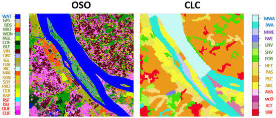
Figure 3 illustrates some of the semantic discrepancies observed between both maps. First of all, one might notice that CLC distinguishes marine from inland waters with an arbitrary boundary well visible in this subset. Such an artificial decision is of course not transferable without either knowing the rule behind the decision or using a contextual translation framework. We also see a CLC polygon of inland wetland on the middle island, corresponding to Woody Moorlands in the OSO nomenclature. This case is difficult due to the lack of semantically close class for Wetlands in the OSO nomenclature. This calls for integrating contextual information. As a final example, one might notice that the agricultural areas on the riversides are partly misclassified in OSO as Continuous and discontinuous urban areas. This error is often observed in the OSO data set on permanent crop areas. A contextual framework should be able to give a correct translation despite the confusion, noticing that permanent crops are also partly detected in the OSO map.
However, one must keep in mind that context only helps translation but can not achieve by itself perfect translation. A good illustration is provided by land-use translation. This is a notoriously difficult challenge for a remotely sensed map such as OSO since it involves predicting land-use from land-cover. A context-wise approach might help: spatial context closely relates to land-use. Figure 4 gives an example of Artificial non-agricultural vegetated areas (AVA) correctly translated from Broad leaved forest. This small forest was located in a city, leading to assign a green urban area label. This example is of interest since it shows two main limitations of our method. First of all, those areas tend to be underestimated (marked bottom area) since predicted AVA areas are often erroneous. Therefore, the network tends to translate into AVA when the AVA likelihood is very high. Secondly, in CLC level 2, no difference is made between Sport and leisure facilities and Green urban areas (all classified as AVA). Thus, the 25 ha MMU of CLC might induce confusion when analyzed on the level 2 product. For example, the marked middle area is a stadium too small to be referenced as a Sport and leisure facilities in the CLC level 3 nomenclature. Therefore, it is generalized and appears as an Urban fabric in CLC level 2. On the opposite, our method, which analyses the same way Green urban areas and Sport and leisure facilities (they are all AVA), translates it as an AVA. Note that Green urban areas are always inside or near cities, which is far from being the case of Sport and leisure facilities. Since we proceed at level 2 (they both are AVA), the spatial context analysis remains difficult. All those observations are generalizable to other land-use classes (Mine/Dump/Construction sites or Industrial, commercial and transport units).
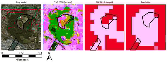
Figure 4.
Limitation of a context-aware translation. Example of Artificial non-agricultural vegetated areas. Satellite image extract from Bing Aerial ©2021 Microsoft Corporation ©2021 Maxar ©CNES (2021) Distribution Airbus DS.
For full France, we obtain an overall agreement of 73% between CLC 2018 and the derivation of CLC from OSO, based on the pure semantic 1 → 1 translation. Without integrating spatial knowledge and more complex class relationships, we show that correct results can be obtained despite random and systematic errors of both data sets. This provides a baseline and an order of magnitude of the expected accuracy with a supervised spatio-semantic approach. Figure 5 provides an alternative point of view of the observed associations between OSO and CLC maps. It shows the proportion of each OSO class associated with each CLC class. The color saturation and the size of the squares indicate this proportion. When the observed association matches the semantic association, the square is blue. Otherwise, it is red. For example, the OSO class road surfaces is mainly associated with the CLC class arable (the most prominent and brightest square in the line) while this association is semantically inconsistent (red). Integrating spatial knowledge into a translation framework should therefore go further than simple pixel-to-pixel or polygon correspondence between both maps.
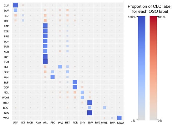
Figure 5.
Observed associations between OSO and CLC (Hinton diagram). The association is computed by resampling CLC to a 10 m raster using the nearest-neighbor approach. We then perform a direct comparison between OSO and CLC. Blue and red colors indicate an agreement and a disagreement between the semantic and the observed relationship between two labels, respectively.
A second challenge comes from the fact that the classes are not balanced. For instance, in the CLC map, the ratio between the most and the least represented classes is higher than 200 in level 2 and higher than 7000 for level 3. Learning the translation from unbalanced data may lead to missing associations due to under-represented classes.
A third challenge is to mimic the CLC MMU. Indeed, the transformation from a 10 m raster map to a map with a 25 ha MMU is not straightforward. A correct translation requires learning the generalization procedure of CLC. It requires proposing a spatial context-aware translation framework that learns rules such as: “If two adjacent areas of discontinuous and continuous urban fabric occur, each of them <25 ha, but in total >25 ha, they should be mapped as one single polygon, and discontinuous urban fabric is privileged”.
Finally, the translation has to handle errors in both land-cover maps. The OSO products have an 89% overall accuracy while CLC 2018 accuracy on level 3 product is estimated to 94.2% over France (the value for level 2 is unknown but should be close, [47]). A per-class analysis of the OSO product enables us to forecast which CLC labels are bound to be mistranslated. For example, OSO Road surfaces and Industrial and Commercial units tend to be underestimated. Thus, the CLC class Industrial, commercial and transport units is expected to have a low recall. Similarly, some CLC classes exhibit limited accuracies (Mine, dump and construction sites or Heterogeneous agricultural areas), which is also detrimental to the learning process.
3.3. Land-Cover Translation Scenarios
Unlike traditional semantic-based methods, a learned translation requires that both source and target map samples exist. Unfortunately, a time gap is often observed between source and target generations, constituting a significant constraint for operational uses. We propose three different scenarios corresponding to different time gaps between source and target land-cover maps, and subsequently to three distinct operational use cases. As stated above, we selected two reference years for CLC (2012 and 2018) and two for OSO (2016, 2018). The goal is to use OSO to produce yearly updates of CLC. From the various association combinations, we retain three scenarios for the assessment of the land-cover translation methodology presented in Section 4.
Scenario 1 consists of using OSO 2018 and CLC 2018. This is the only pair of products we have with the same reference year. The use case corresponds to an automatic extension of CLC to a broader area, since, for instance, CLC has not yet been generated over a full area of interest (Figure 2E). This is particularly relevant for the forthcoming editions of CLC: one would only need to generate a sample high-quality version on specific areas and our framework could fill the gaps.
Scenario 2 corresponds to the updating operational setting. First, a translation model is trained on a pair of existing OSO and CLC products. Then, the model is applied on the OSO product of the year for which the new CLC map is to be produced. We assume that the most recent OSO product is 2018 and that we want to produce CLC 2018. The translation model is trained using CLC 2012. We choose to pair it with OSO 2016 to minimize the disagreement in the training data caused by land-cover changes. In this scenario, OSO 2018 is translated with the learned model, and CLC 2018 will be used as reference data for validation.
One criticism that can be made about Scenario 2 is that if the learning algorithm can cope with discrepancies in the training data, it may be better to use the most recent OSO map in the training phase. This would allow taking into account the evolution of land-cover, which does not affect the translation itself. For instance, one could assume that climate change makes wetland areas dryer. This would not introduce a change between CLC 2012 and CLC 2018 (dryer wetlands are still wetlands) but could introduce an evolution in OSO. Indeed, OSO does not have wetland classes, and wetlands in CLC correspond to water, sand, grasslands or moorlands in the OSO nomenclature. In this situation, some CLC wetlands could transition from water to sand, grassland or moorland. This would mean that the translation rule learned between OSO 2016 and CLC 2012 could not be applied to OSO 2018.
In order to assess this situation, we propose the Scenario 3 on which the translation model is trained by pairing CLC 2012 with OSO 2018. This model is then applied to OSO 2018. CLC 2018 is used for validation. The underlying assumption is that the model will fail to learn some of the associations imposed by the training data that correspond to real changes from the point of view of the CLC nomenclature.
3.4. Data Set Preparation
We work on the full French metropolitan territory, i.e., French mainland and Corsica island. OSO and CLC are both publicly available on their respective official websites (http://osr-cesbio.ups-tlse.fr/~oso/ accessed on 25 January 2021, https://land.copernicus.eu/pan-european/corine-land-cover accessed on 25 January 2021). OSO is directly downloaded in raster format while CORINE Land Cover is obtained in vector format and then rasterized. Since we need to match the data sets both in terms of cartographic datum and spatial grid, we perform the rasterization step of CLC jointly with this transformation step. We align the two rasters with a simple spatial translation to make sure that the maps are correctly registered at the pixel level. Eventually, since the OSO 2016 nomenclature merges most of the agricultural classes into two super classes, namely, summer crops and winter crops, we perform similarly for the OSO 2018 products. This step is only mandatory for Scenario 2 but is still applied to all scenarios to make them comparable.
4. Deep Learning Based Map Translation
As stated in Section 2, the main current translation solutions are manually defined or require at least the explicit knowledge of the semantic transformation between classes of the two land-cover maps. This approach does not offer sufficient versatility and narrows down the translation cases that can be handled (as shown in Section 3.2). Consequently, to overcome such limitations, we propose a machine learning approach that automatically learns such a transformation in a supervised way. Our method simultaneously performs semantic and spatial resolution translations to take into account the entanglement of the two types of information. We use existing pairs of source and target land-cover maps, which provide large volumes of training data. We adopt an approach based on Convolutional Neural Networks (CNN) since they are perfectly tailored to integrate the semantics of the pixel with its spatial context and are therefore appropriate for the task at hand.
4.1. The Proposed Neural Network Architecture
Land-cover classification is traditionally cast as a semantic segmentation task, in which a set of remote sensing images are transformed into a class map [51,52,53]. The land-cover translation task can also be seen as a semantic segmentation task where the input pixels are not physical values (namely, the optical spectral bands or SAR polarized channels), but semantic classes, i.e., nominal categorical data with low cardinality.
One difference between the land-cover classification and translation challenges is that the former usually keeps the spatial resolution of the input data, while the latter often requires to produce an output with a different resolution (see Section 2 and Figure 2).
We choose to use the popular U-Net encoder-decoder architecture [54]. The main idea of U-Net is to encode the image input into a vector representation using successive down-sampling and convolution steps and then restore (decode) the image using successive up-sampling and deconvolution layers (see Figure 6). Skip connections between the symmetrical layers of the encoder and the decoder are used to avoid losing spatial information due to the down-sampling process. However, this does not alleviate the main limitation of the standard U-Net formulation: its symmetry imposes aggregating features of the same scale in the encoder and decoder sub-networks, which forbids the change of resolution. Choosing different ratios for the down-sampling and the up-sampling parts allows taking into account this change between the input and output maps. We propose the following adaptation. Let r be the resizing factor between the input and the output of the network, and the downsizing factor of the different pooling layers in the encoder. We need to ensure that:
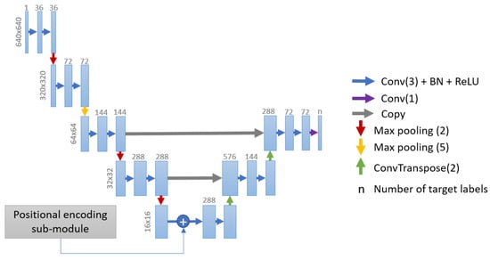
Figure 6.
Our U-Net adaptation. An asymmetrical encoder-decoder is designed so as to efficiently handle the distinct spatial resolutions of the source and the target.
Pooling parameters must be as small as possible to reduce the loss of spatial detail.
This problem has one unique solution, which can be obtained by prime decomposition [55]. In our case, the target map is 10 times smaller than the source map. This leads to apply five and two pooling layers in the asymmetrical part of the encoder. To avoid information loss, we apply the two pooling layers first.
To be able to feed this CNN with OSO and CLC, we slightly modify the input data. We first split them into 14,705 source/target couples of patches of 6400 × 6400 m size for GPU memory concerns. Secondly, we make the network return one hot-encoded prediction of the map, instead of a simple prediction, to be able to adopt usual loss functions.
4.2. Geographical Context
It is widely assumed in the literature that inserting the geographical context into CNN architectures helps to improve the semantic segmentation task [56,57]. Here, we hypothesize that the translation of a land-cover element may co-variate with its spatial coordinates (latitude and longitude). This assumption is in line with the current practices in large-scale land-cover classification approaches in the remote sensing community: it is implicitly performed by either locally fine-tuning a global classification model or by defining distinct local models based on a specific stratification strategy [44,58]. Thus, we decide to incorporate into our network a positional encoding sub-module to take into account the coordinates of each patch during the translation process. Previous attempts have been made to improve CNN-based classification of terrestrial images using various embedded features [59]. The main strategy includes a direct insertion of (quantized) latitudes and longitudes [60] or to retrieve proxy attributes that are more likely to be discriminative (population statistics, social media, see [61,62]. However, to the best of our knowledge, such a strategy has never been proposed for land-cover mapping.
The most natural way is to use the geographical coordinates as a residual connection, adding complementary information to the learned representation. Helping land-cover prediction with 2D coordinates is equivalent to approximating an inherently discontinuous function such as “if (x < 10,000 and y > 50,000) or (x > 500,000 and y < 3500), then it can/cannot be seashore”. Since Multi-Layer Perceptrons (MLP) are known to have issues with approximate discontinuous functions [63], we instead propose to adopt the positional encoder strategy [64], adopted by the transformer architecture, as a way to make the signal more continuous.
Unlike the traditional sequence-to-sequence architecture, here, the positional encoding must be in 2D in order to both integrate latitude and longitude. The authors of [65] proposed a strategy for image coordinates: rows and columns are independently encoded and then concatenated. We adopt the same strategy with the latitude and longitude coordinates. Let x and y be the longitude and latitude, respectively, is the corresponding positionally encoded matrix and d the dimension of the encoded matrix, which corresponds to the number of feature maps generated by the CNN layer where the positional encoding is added.
The resulting encoding is given to a one layer perceptron to preprocess the positional encoding. Note that adding more layers did not show significant improvement in our results. The output is added to the bottleneck of our U-Net in so that the positional information has only influence at a coarse scale.
4.3. Loss Function
The standard loss for semantic segmentation tasks is binary cross-entropy (BCE). It is defined as a measure of the difference between two probability distributions for a given random variable or a set of events. Let p be a softmax prediction of the network and y the ground truth, with the predicted probability of class i and if the correct class is i and otherwise. The BCE loss is computed as:
The principal limitation of BCE is that it does not suitably handle imbalanced classes. As stated previously, our case study holds highly imbalanced data, which prevents its adoption. Many approaches have been proposed [54,66,67] to cope with the class imbalance issue, such as the weighted cross-entropy [68] or focal loss [69]. Additionally, region-based losses target to maximize the overlapping ratio between p and y. Among all these losses, we select the Dice loss [70]: it computes an approximation of the F1-score metric, which is vastly used in the remote sensing community. The Dice loss is computed as follows:
We combine the BCE and the Dice loss, as suggested in [71,72,73,74], to incorporate benefits from finer decision boundaries (Dice) and accurate data distribution (BCE). This alleviates the problem of high variance of the Dice loss.
4.4. Quality Assessment
The quality assessment of a map can be qualitative and quantitative. The qualitative assessment focuses on three distinct features, based on a comparison between the predicted map and the reference one:
- General aspect: does the translated map look like the reference one?
- General quality: are any classes under or over-estimated?
- Geometric preservation: is the shape of each predicted structure in the map close to its reference counterpart? Which shapes are harder to translate?
The quantitative assessment relies on a reference data set. We first randomly split the previously mentioned 14,705 couples of patches into disjoint train, validation (a small set used during the training of the network to watch for convergence) and test data sets, accounting for, respectively, 50%, 10% and 40% of patches.
The quantitative evaluation was conducted using traditional quality metrics derived from the confusion matrix (Overall accuracy, F1-score, Kappa). Metrics were computed on 10 different initializations and trainings of our network. Mean values and the corresponding standard deviations are displayed in this paper.
As stated before, the target map used for training can have errors and therefore, quality metrics computed with these data can be misleading. In order to alleviate this, we manually annotated the center pixel of the 6022 test patches. The class given in the CLC 2018 map was visually validated and corrected if necessary. We used 10 m Sentinel-2 2018 satellite images and 1 m Bing aerial images to disambiguate complex cases. We respected the Minimal Mapping Unit of 25 ha of CLC.
The comparison between CLC 2018 and our reference version of CLC 2018 gives a 86% match. This fits with the specifications of the CLC product, which is 85%. We did not create the ground truth from scratch but only by correcting CLC 2018: there may be a bias towards a high agreement with CLC. Table 3 provides some statistics about the reference data set with respect to the CLC classes, as well as the associated precision, recall and F1-score.
Table 3.
CLC statistics on our reference dataset. See Table 2 for the class codes.
The manually validated center of test patches, which we will refer as ground truth, was obtained by random selection while preserving the initial imbalance of classes in CLC. Therefore, some categories are very rarely represented (e.g., Mine/construction/dump sites are only observed five times), while others are over-represented (e.g., Arable land appears 1685 times). To overcome this issue, one might want to annotate more samples, but this entails significant time costs and leads to higher class noise. Indeed, rare classes are often complex to discriminate even using very high spatial resolution images and multisource time series.
Note that our evaluation strongly differs from the official CLC 2018 evaluation procedure [47], from which a 94.2% accuracy was obtained for CLC level 3 over France (versus our 86% on level 2). This stems from multiple variations between the CLC quality assessment protocol and ours:
- Two different operators double-checked the CLC official validation dataset while ours includes only one interpretation for each point.
- The official validation is achieved with respect to the CLC initial segmentation (to avoid taking into account geometric errors, separately evaluated), while ours corrects wrong segmentations. Therefore, our interpretation of the same point might differ on edges.
- The official validation is performed on the vector data while ours is performed on a rasterized version, which tends to amplify CLC segmentation errors.
Since we do not have access to the CLC validation dataset, all metrics are computed on our ground truth. Thus, we will not target the 94% accuracy but the 86% observed on our dataset.
Evaluating the quality of the geometric preservation of a map is rarely done in land-cover classification studies. Thus, we lack predefined quantitative measures to assess it. We propose to use the Edge Preservation Index (EPI), traditionally used in image reconstruction or denoising [75,76]. It computes the correlation between edges in a pair of images. EPI is defined as [77]:
where p is the map predicted by the network, t is the ground truth target, denotes a high pass filter (we use a simple Laplacian kernel), denotes the mean of the high pass filtered image, and is defined as:
where and represent the number of pixels in rows and columns respectively of the given image.
Since we work on categorical data, edges are discretized (0 = non edge, 1 = edge). Ideally the EPI should be computed between our prediction and perfectly segmented ground-truth version of CLC 2018. Since the creation of this perfect segmentation would be overly time consuming, we simply compute the EPI between our prediction and CLC 2018. Thus, it shows the agreement between the prediction and CLC edges rather than the true correlation between our prediction and a perfect segmentation. The larger the EPI value is, the more edges are maintained. From the analysis of our data, we propose the following interpretation key for EPI value. EPI is inferior to 0.1 when no boundary agreement exists. A limited match between edges leads to 0.1 < EPI < 0.5. Conversely, 0.5 < EPI < 0.9 indicates a correct boundary association and 0.9 < EPI < 1 corresponds to an almost perfect match.
4.5. Comparison with Other Solutions
To better evaluate the performance of our method, we compare our three scenarios with standard semantic approaches. They usually focus only on nomenclature changes, discarding the modification of the spatial resolution. Three baselines are considered:
- “Naive semantic”: we directly translate the OSO nomenclature into the CLC one. For each OSO class, we associate the closest CLC class by our own expert knowledge. Then, we evaluate the differences between the translation and CLC, based on random points sampled over the full spatial extent of the map.
- “Naive down-sampling”: the second method integrates the change of spatial resolution. The spatial resolution of OSO is 10 m, i.e., ten times superior to CLC. Therefore, we convert a set of 10 × 10 pixels of OSO into one CLC class using a majority vote.
- “Auto-semantic”: the third one translates a set of 10 × 10 pixels of OSO into a single CLC class using a Random Forest classifier. The features are the frequencies of each OSO class in each area of interest, in an Entangled Random Forest flavor. Training is performed on the same training set as the neural network in Scenario 1.
In addition, we also perform an ablation study and generate results using and discarding the CNN module related to the geographical context.
5. Experiments and Discussion
In this section, we investigate the translation performance of our asymmetrical U-Net on the three proposed "OSO to CLC" scenarios (Section 5.1, Section 5.2 and Section 5.3) for all of France. Our method is then compared with simpler solutions (Section 5.1). Links for our code (https://github.com/LBaudoux/Unet_LandCoverTranslator accessed on 25 January 2021) and dataset (http://doi.org/10.5281/zenodo.4459484 accessed on 25 January 2021) are provided.
5.1. Scenario 1
Figure 7 presents a sample of diverse areas, selected from our France-wide translation.
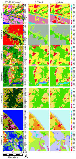
Figure 7.
Various results of our translation framework obtained over France for the three scenarios. Each area is 41 km wide. Scenario 2 results on all of France are available at https://oso-to-clc.herokuapp.com/ accessed on 25 January 2021.
The qualitative analysis first reveals that the results are visually very satisfactory. Errors in the translation mostly occur on CLC classes with no semantically close class in OSO (namely, Mine and construction or Wetlands), which was expected. Such a limitation cannot be addressed without external knowledge. Furthermore, one might notice errors on linear shaped structures (like the road in the second row of Figure 7). There are two possible factors. The first one is that U-Net architectures are known to perform poorly on linear segment prediction. The second is that the rasterization step of our data set creation procedure may lead to the disappearance of tiny linear features: they are too small to be represented in raster maps with a spatial resolution of 100 m. Consequently, some roads and small water sections are removed from the (training) data set, making the prediction of such structures more difficult. In addition, our predictions inherit systematic errors of the OSO product. For example, the OSO classes Mineral surfaces, rocks tend to be overestimated on mountain areas, resulting also in an overestimation in the CLC prediction of the non vegetated natural class. Finally, systematic errors exist on the border of the patches due to the local lack of information.
These qualitative observations are quantitatively confirmed (Figure 8). Our first observation is that precision and recall are nearly equivalent for most classes making the method balanced. From the analysis of the confusion matrix, one might notice that the largest confusion observed is that most predicted inland wetlands are in fact inland waters. This underlines the fact that on CLC classes with no OSO corresponding class, confusion unavoidably happens with close CLC classes. It appears impossible to improve the discrimination power of our method on this class without adding extra information. Additionally, some CLC classes such as Heterogeneous agricultural areas and Artificial non-agricultural vegetated areas are confused with a large number of other CLC classes; revealing both the need of extra information to disambiguate OSO data and the complexity of those two CLC classes (one merging multiple CLC classes, the other mixing land-use and land-cover).
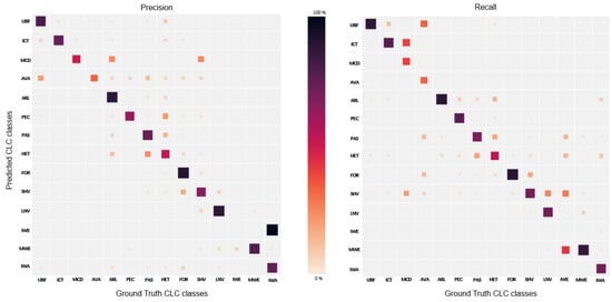
Figure 8.
Confusion matrices between prediction and ground truth. Left: expressed as prediction proportion. Right: expressed as ground truth proportion. The diagonals provide the per-class precision and recall, respectively.
Using the manually labeled reference data, the obtained overall accuracy is 81%. This is slightly under the specification of CLC (>85%), under the official estimated accuracy of CLC (94.2%), and under the accuracy of CLC on our ground truth data set 86%. A detailed per-class quantitative analysis is provided in Figure 9.
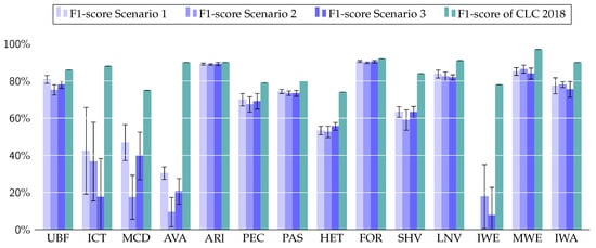
Figure 9.
Mean F1-score obtained for 10 different initializations of the network for each scenario. Error bars indicate the standard deviation over the 10 trials.
The best translation performances are obtained for Urban fabric, Arable land, Permanent crops, Forest, and Non vegetated natural. The class Maritime water does not change over the various editions of CLC. We decided to provide to the network a mask for this class to ensure it focuses on finding wetlands and water bodies only. A perfect score is reported for this class but is meaningless for our analysis.
We can draw the following observations:
- Urban Fabric, Arable land, Forest and Open spaces with little or no vegetation achieved a very high F1-score with, respectively, 0.84, 0.89, 0.91, and 0.82 values.
- The class Coastal wetland obtained a high 0.83 F1-score despite being absent in OSO. This is partly explained by the fact we provided a marine water mask to the network helping the contextual translation over such areas.
- Artificial non-agricultural vegetated areas is the class with the lower F1-score (0.3). This can be partly explained by the fact that this class mainly refers to land-use categories (green urban areas/sport and leisure facilities), out of OSO classes. This class could be recovered with contextual information by increasing the size of the receptive field (e.g., stadiums have distinguishable shapes). However, this would be detrimental to a correct shape retrieval for other classes.
- Mine/Dump/Construction sites obtained a 0.5 F1-score despite having no clearly defined semantically close class in OSO. OSO maps usually mix a lot of classes on those areas, giving them a unique and contextually recognizable texture to translate.
- Heterogeneous crops are difficult to predict since the class corresponds to a mix of several OSO classes, explaining their limited F1-score (0.55). Thus, it is not surprising that it performs worse than most classes. Again, it can only be determined through contextual analysis.
- Industrial, commercial and transport units (ICT) are poorly predicted while close semantic correspondences exist with OSO Industrial and commercial units and Road Surfaces. Working with the full 23 OSO labels (decomposition of Summer crops and Winter crops into a more detailed crop nomenclature) fosters a vast uprising of the ICT F1-score from the observed 0.44 to 0.7. Thus, we hypothesize that the observed low value stems from errors in the OSO data (some of the ICT being confused with crops).
As stated previously, accuracy metrics for the classes Mine/dump/construction, Artificial non-agricultural vegetated areas and inland wetlands are computed on a small number of reference samples. In Appendix B.1, we give a comparison between the observed F1-score agreement computed between our prediction and CLC 2018 and the previously presented F1-score computed between our prediction and our ground truth. Since CLC 2018 is not error-less, the computed values are not as reliable as the ones we compute with our ground truth. However, statistics can be computed on the whole test set and are therefore much more comprehensive.
Class overestimation or underestimation are provided in Table A2 with the ratio between the total per class area in our translation and CLC 2018. We also give per-class accuracy and precision. We show that well-classified classes are overestimated and that, conversely, poorly classified classes tend to be underestimated: our network indeed tends to avoid making errors. However, other factors can have a per class impact on over and underestimation. For example, the only class with high metrics being slightly underestimated is Arable land. We attribute this behavior to the fact that, to maintain a correct loss on Heterogeneous agricultural areas, the network tends to degrade the loss on Arable land, thus inducing this slight underestimation.
A special focus must be made on the three land-use classes (Industrial, commercial and transport units, ICT, Mine/dump/construction, MCD, Artificial non-agricultural vegetated areas, AVA). They tend to be the most difficult to predict from OSO, which is a remotely sensed map. While ICT is partly detailed in the OSO nomenclature (while being significantly erroneous), MCD and AVA have no semantic correspondent. Interestingly, our method remains able to partially predict some of them. For example, some AVA (green urban areas) are located in urban areas and thus can sometimes be predicted from OSO labels, such as Broad leaved forest or Natural grassland (see Figure 4). However, the task remains challenging mainly because spatial context is often not discriminant: camping sites or golf courses are mostly grasslands often outside cities for which spatial context is of little use for translation. Thus, to improve land-use class discrimination, additional data are required. While being straightforwardly integrated into our network, we discarded such solution and focused on pure context-based translation.
The Edge Preservation Index in this scenario is equal to 0.44. This might be first explained by the fact that both the true CLC and our predicted CLC tend to be more erroneous on edges. Secondly, the difficulty in predicting linear structures participates in such a low value. Thirdly, highly segmented areas correspond to specific classes where our method is prone to fail (e.g., Heterogeneous agricultural areas).
5.2. Scenario 2
In this scenario, we use our proposed translation framework to train a network with the first available OSO land-cover map (2016) as source and CLC 2012 as target. In the prediction step, we feed the network with OSO 2018 aiming to obtain CLC 2018.
Results are very similar to the ones observed in Scenario 1. All qualitative observations made previously still hold. Thus, we focus here on the analysis of particular cases to show limitations not discussed before.
The first row of Figure 10 illustrates the case of a lack of semantic distinction between two classes (here between Shrubs and Forests). CLC tends to recover more shrub areas than OSO, where they are more likely to be classified as forests. Consequently, our network fails in perfectly translating CLC Shrub and/or herbaceous vegetation association areas. The second row shows an example of a segmentation differing between our prediction and CLC. The segment is classified in CLC as Heterogeneous agricultural areas: it mixes both Arable land and Pastures with no dominating land-cover. Our prediction exhibits another segmentation by discriminating separately Arable land and Pastures. This seems reasonable according to the source OSO map even though differing from the CLC one. This is the limitation of translation frameworks: we may hardly learn map specifications and cope with existing errors.
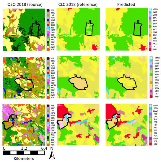
Figure 10.
Several failure cases for the Scenario 2. Note that other areas are correctly recovered. See text for more details.
The third row shows an example with unpredictable classes due to the lack of semantic and contextual information. The network has to translate the OSO Intensive grassland into the CLC artificial non agricultural vegetated area class. Since the former one more relates to land-use than land-cover, the semantic association is weak. At the same time, contextual knowledge does not foster information extraction since Intensive grassland near cities will most of the time correspond to a Pasture or Heterogeneous agricultural areas in the CLC nomenclature.
A per-class quantitative analysis is provided in Figure 9. We obtained an overall accuracy of 79%. This is slightly below the 81% score observed in Scenario 1. The comparison between the F1-scores obtained in both scenarios shows that Scenario 2 exhibits significantly worse results on artificial surfaces. No change is observed between Scenarios 1 and 2 on best translated classes: Arable land, Permanent crops, Forests. Note that the small number of points in our ground truth prevents a deeper analysis.
Multiple reasons may explain the 2% under-performance of Scenario 2. One reasonable hypothesis is that the under-performance is a consequence of a variation between OSO 2016 and OSO 2018 products. In fact, OSO 2016 differs from 2018 by its 1% smaller accuracy and fewer classes (some crop classes are merged).
5.3. Scenario 3
Qualitative analysis shows that the Scenario 3 results are very similar to those obtained in the two former configurations.
Quantitative analysis confirms our previous observations (Figure 9). Scenario 3 achieved an 81% accuracy, in line with the per-class F1-score of Scenario 1. A single class reaches a significantly lower accuracy: Industrial, commercial and transport units (0.18 instead of 0.42 and 0.38 in Scenarios 1 and 2). This may be due to changes between 2012-2018, exacerbated by the limited initial consistency between both data sets and few validation points.
Note that the Edge Preservation Index remains stable at 0.44 in this set-up. This is a relatively low value for a prediction being between 73% identical to CLC 2018. This is simply explained by the fact that most discrepancies between CLC and our prediction are observed on edges (see Section 5.1).
5.4. Comparison with Other Solutions
In this subsection, we compare our method with the previously mentioned semantic baselines. Figure 11 shows the results of the various solutions with respect to the ground truth on a highly challenging area (41 km). Qualitatively, the first observation is that non-contextual translations (naive semantic, naive down-sampling, and auto-semantic) unsurprisingly failed to retrieve the CLC MMU, leading to a noisy output. However, note that even though our approach better translates CLC MMU, it still tends to include objects that are too small. For instance, we measure that almost 5% of our method translated <25 ha areas (against 0.3% in the used rasterized version of CLC). Non contextual translations also generated less diverse classes than our proposed solution for various reasons. First of all, naive semantic and naive down-sampling solutions cannot predict classes with no semantically close classes like Wetlands. Secondly, several classes like Heterogeneous agricultural areas cannot be predicted without taking into account an adequate spatial support.
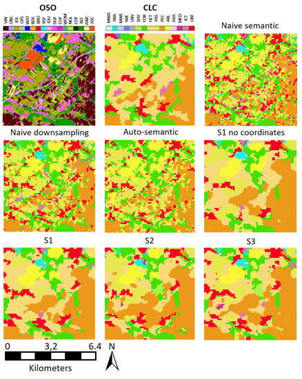
Figure 11.
Visual comparison between the different experimented scenarios (S1-S2-S3), with and without the geographical sub-module (‘S1 no coordinates’), and with baselines methods.
Note that the qualitative comparison between our network with and without the coordinates sub-module reveals little to no change (called ‘S1 no coordinates’ and ‘S1 no C’ in Figure 11 and Figure 12).
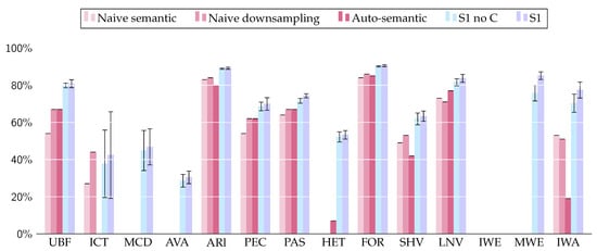
Figure 12.
F1-score of each solution. Error bars indicate the standard deviation over the 10 trials for machine-learned methods. ‘S1 no C’ stands for ‘Scenario 1 without the geographical sub-module’.
Quantitatively, our network gives around 10% higher metrics than traditional methods (see Figure 12 and Table 4). The superior results of our approach can partly be explained by the ability of the network to output realistic maps even when no semantically close class exists (e.g., Wetlands). Furthermore, one must notice that the proposed approach outperforms non contextual methods on each class and not only on classes with no semantically close classes. Interestingly, we observe that the addition of the coordinate sub-module slightly increases the quantitative performances for almost all classes. The highest gains are observed in classes only present on some parts of the territory (cities, wetlands, heterogeneous crops). The increase is particularly noticeable on Maritime wetlands and Inland waters for which the addition of coordinates acts like a reliable filter function. However, the global increase is too small to achieve statistical significance and qualitative changes. Note that the EPI of contextual translations is higher than non contextual ones. This can partly be explained by the inability of non-contextual frameworks to translate the MMU of CLC.
Table 4.
Comparison with traditional non contextual approaches and ablation study. Best results are highlighted in bold.
6. Discussion
This paper proposed a novel method for the yearly production of CLC maps from higher resolution OSO maps. To do so, we defined a translation framework able to handle both the semantic and spatial resolution of the source map to match the target one. Through a literature review, we first discussed existing methodologies based on separate semantic or spatial translations. We identified that the three main limitations of the literature were that the spatial context of each object was not taken into account, that semantic relationships were often manually established and that spatial and nomenclature shifts were performed separately.
To achieve sufficient performance, we proposed a fully-supervised framework to contextually and simultaneously translate land-cover maps. We performed experiments at country-scale and comprehensively assessed the performance of our approach. We showed that it outperforms current solutions and provides a strong baseline for subsequent improvements.
Unlike traditional semantic methods, our learned strategy requires the existence of both source and target maps. We studied the impact of the time gap between source and target through three different scenarios, corresponding to three operational use cases.
Our first scenario consists of translating OSO 2018 into CLC 2018. The obtained model can then be used to generate CLC on unseen areas (completion strategy). We obtained an overall accuracy of 81% based on a manually-generated ground truth. It surpassed existing methods. Unfortunately, results remain inferior to CLC specifications and official accuracy (85% and 94.2%, respectively), which leaves room for improvement. Effort on geometric accuracy (boundary definition) and on mixed land-use/land-cover classes improvement is still needed to achieve higher accuracy. We believe that the combined integration of multiple source maps could be relevant to disambiguate specific confusions. This would require a multiple-stream network to benefit from the discriminate power of each map.
Our second scenario consisted of training a model to translate OSO 2016 into CLC 2012 and then use this model to translate OSO 2018 into CLC 2018, i.e., to generate an updated version of CLC. We achieved a 79% accuracy, slightly under-performing the first scenario, especially on urban classes. This could partly be explained by the difference between the OSO 2016 and 2018 products in terms of per class thematic accuracy. Additionally, this could also partly be explained by the difference between the regularization needed to correct land cover changes between OSO 2016 and CLC 2012 versus OSO 2018 and CLC 2012. This method could be once again improved using multiple maps to reduce over-fitting: this would help us increase even more the agreement between our prediction and CLC 2018.
Our third scenario simply tries translating OSO 2018 into CLC 2012 with the underlying hypothesis that changing areas between 2012 and 2018 will only be considered as additional noise. We achieved a performance qualitatively and quantitatively similar to the first scenario (81%). Thus, this scenario achieves a fairly good result while not needing a common time stamp of the source and target for learning (scenario 1) and no older source map (scenario 2).
The analysis of the results of the three scenarios reveals that in our application context (a low resolution target map), the time-step between the source and the target maps does not negatively influence the performance of the approach if it remains reasonable (6 years in this study). Note that interestingly this statement seems to hold for all classes. Our framework therefore proposes a realistic approach for the generation of the next versions of CLC.
It offers the possibility to produce a CLC map at the country scale from an existing map in less than 1 day, using 14,705 patches, with a consumer-grade computer (8 CPUS and a Nvidia V100 GPU). Training takes approximately 10 hours and inference is achieved in less than 30 min. Note that if no OSO map is available, it can be generated in less than a week. Therefore, the whole procedure (OSO generation and translation into CLC level 2) takes less than a week, making this method time competitive. A yearly generation at the European scale is therefore conceivable.
The method worked particularly well on the most represented land cover classes, i.e., Urban, Forest, and Arable land. However, some challenges remain. First of all, our method performed poorly on the edges of objects and (thin) linear structures. A more adapted method should be used to preserve these structures. Thus experiments on boundary loss must be conducted to improve the results on those structures. Furthermore, even though the contextual framework helps translating classes when no clear n→1 semantic relationship exists, the result may remain insufficient to match the target specifications. To achieve expected accuracy, large score improvements are needed on land use classes, which seems impossible without the use of additional data. Finally, the method is currently unable to give satisfactory results on CORINE Land Cover level 3 nomenclature: it mixes land-use classes with land-cover ones. This problem can be hardly solved without adding extra information and thus involves a modification of the technique proposed here to fuse different types of data. Simply extending the spatial support of our analysis might result in better capturing the context necessary to discriminate land-use classes and it is likely to be detrimental to linear structures and small elements.
We believe in the high potential of spatial-semantic translation of land-cover maps to support new applications in inter-operating land-cover data sets. Our method also offers the advantage of generating maps with multiple variations of a nomenclature without requiring remote sensing images and with a quality almost similar to the map specification. Unlike previous approaches, contextual translation shows a high capacity to deal with nomenclatures when difficult semantic relationships exist. This also enables to correct some of the errors in the source data set. As a current limitation, our method works only when source and target maps spatially overlap, which might prevent some key applications related to map transfer. Therefore, some effort must be devoted to proposing a non-fully supervised method for contextual translation.
Author Contributions
L.B. is the main author of this manuscript, he designed and implemented the experimental framework and contributed to the analysis of the results. J.I. and C.M. defined the requirements, oversaw the process and participated in the analysis of the results. All authors reviewed and edited the manuscript. All authors have read and agreed to the submitted version of the manuscript.
Funding
This research was supported by the AI4GEO project (http://www.ai4geo.eu/ accessed on 25 January 2021.) and the French National Research agency as a part of the MAESTRIA project (grant ANR-18-CE23-0023).
Institutional Review Board Statement
In this section Not applicable.
Informed Consent Statement
Any research Not applicable.
Data Availability Statement
In this section The dataset presented in this study is openly available in ["Oso to Corine Land cover dataset", Zenodo] at http://doi.org/10.5281/zenodo.4459484 accessed on 25 January 2021. The code presented in this study is openly available at https://github.com/LBaudoux/Unet_LandCoverTranslator accessed on 25 January 2021 France wide result for scenario-2 is openly available at https://oso-to-clc.herokuapp.com/ accessed on 25 January 2021.
Conflicts of Interest
The authors declare no conflict of interest.
Appendix A. Data Set
Table A1.
Semantic association between OSO and CLC. The second column informs on the percentage of the data effectively following this association.
Table A1.
Semantic association between OSO and CLC. The second column informs on the percentage of the data effectively following this association.
| OSO Classes | CLC Classes | Observed |
|---|---|---|
| Dense urban | Urban fabric | 87% |
| Sparse urban | 45% | |
| Industrial and commercial | Industrial/Commercial/transport | 14% |
| Roads | 16% | |
| Rapeseeds | Arable land Heterogeneous agricultural areas | 91% |
| Cereals | 90% | |
| Protein Crops | 91% | |
| Soy | 91% | |
| Sunflower | 89% | |
| Maize | 83% | |
| Rice | 96% | |
| Tubers | 96% | |
| Orchards | Permanent crops Heterogeneous agricultural areas | 62% |
| Vineyards | 82% | |
| Pastures | Pastures Heterogeneous agricultural areas Artificial non-agricultural vegetated areas | 69% |
| Lawn | Shrub and/or herbaceous | 39% |
| Shrub | 41% | |
| Broad leaved | Forest Artificial non-agricultural vegetated areas Heterogeneous agricultural areas | 82% |
| Coniferous | 79% | |
| Mineral surfaces | Open space with little or no vegetation Mine/Dump/Construction | 86% |
| Sand | Open space with little or no vegetation | 65% |
| Glaciers and snow | 100% | |
| Water | Inland water Marine Water | 84% |
Appendix B. Scenario 1
Appendix B.1. Agreement between Prediction and CLC 2018

Figure A1.
Mean F1-score computed between prediction/CLC 2018 and prediction/Ground Truth for 10 different training. Error bars indicate standard deviation on the 10 trainings. Since CLC 2018 is not error-less, the displayed value should not be considered as ground truth values.
Figure A1.
Mean F1-score computed between prediction/CLC 2018 and prediction/Ground Truth for 10 different training. Error bars indicate standard deviation on the 10 trainings. Since CLC 2018 is not error-less, the displayed value should not be considered as ground truth values.

Appendix B.2. Comparison between Predicted Areas
Table A2 shows the precision, recall, and ratio between predicted area and CLC 2018 area for each class. We assume that the CLC 2018 total area per class can act as a reference for the total area covered by each class. High recall and precision classes tend to cover more area than the same classes in the CLC 2018 map, and they are probably overestimated. On the contrary, incorrectly classified classes tend to be underestimated. This seems easily understandable: the network will generate labels on which fewer errors are made.
Table A2.
Per class precision, recall (computed on ground truth) and ratio between predicted area and CLC area.
Table A2.
Per class precision, recall (computed on ground truth) and ratio between predicted area and CLC area.
| UBF | ICT | MCD | AVA | ARl | PEC | PAS | HET | FOR | SHV | LNV | IWE | MWE | IWA | |
|---|---|---|---|---|---|---|---|---|---|---|---|---|---|---|
| Precision on ground truth (%) | 77 | 70 | 56 | 40 | 89 | 65 | 73 | 55 | 86 | 67 | 88 | 0 | 71 | 73 |
| Recall on ground truth (%) | 85 | 37 | 42 | 26 | 89 | 75 | 69 | 53 | 92 | 61 | 79 | 0 | 85 | 66 |
| area Predicted/ area CLC (%) | 113 | 63 | 72 | 65 | 93 | 113 | 106 | 104 | 101 | 106 | 78 | 36 | 125 | 106 |
Appendix C. Role of the Coordinates Sub-Module
In this subsection, we investigate the impact of using the geographical coordinates of each patch on the result. The coordinates sub-module improves the agreement accuracy of 1.5% between our prediction and CLC 2018. Figure 12 shows the per-class F1-score with and without the coordinates sub-module. For most classes, the agreement F1-score is slightly higher when the coordinates sub-module is used, while the difference is not significant enough. Figure A2 presents the mean kappa agreement over France between our network without coordinates and CLC 2018. A quality gradient can be observed clearly following a southwest to northeast direction. The main reasons are:
- Some areas are more complex to translate due to difficult classes and or geometry (small parcels of heterogeneous crops for example).
- Some areas might contain more errors in both source and target data.
- Some classes cannot be obtained without knowledge of the geographical situation. For example, the coastline of Corsica Island (South East) is mostly classified as forests in the OSO nomenclature while being considered as shrubs in the CLC nomenclature. The choice of the shrub class is explained by the fact that forests on the Mediterranean sea coastline are usually low covered. Thus, this translation is impossible from OSO without taking the information of the geolocation into account.
Figure A2 also shows the difference between the mean agreement kappa computed, respectively, with and without the coordinates sub-module. Green areas show where the network with coordinates sub-module outperformed the version without. Thus, we can state that the network with the coordinates sub-module provides better results almost everywhere in France (except for a small portion of the northeast). We see that the improvement is mainly concentrated on southwest France, which was described earlier as the most erroneous zone of the translation. Therefore, we can state that the coordinates sub-modules helps to balance the errors in the data set spatially.

Figure A2.
Mean agreement kappa between prediction without coordinates and CLC 2018 (left). Difference between the mean agreement kappa of the prediction with coordinates and without coordinates (right).
Figure A2.
Mean agreement kappa between prediction without coordinates and CLC 2018 (left). Difference between the mean agreement kappa of the prediction with coordinates and without coordinates (right).

References
- Grekousis, G.; Mountrakis, G.; Kavouras, M. An overview of 21 global and 43 regional land-cover mapping products. Int. J. Remote Sens. 2015, 36, 5309–5335. [Google Scholar] [CrossRef]
- Li, Z.; White, J.C.; Wulder, M.A.; Hermosilla, T.; Davidson, A.M.; Comber, A.J. Land cover harmonization using Latent Dirichlet Allocation. Int. J. Geogr. Inf. Sci. 2020, 1–27. [Google Scholar] [CrossRef]
- Homer, C.; Dewitz, J.; Jin, S.; Xian, G.; Costello, C.; Danielson, P.; Gass, L.; Funk, M.; Wickham, J.; Stehman, S.; et al. Conterminous United States land cover change patterns 2001–2016 from the 2016 National Land Cover Database. ISPRS J. Photogramm. Remote Sens. 2020, 162, 184–199. [Google Scholar] [CrossRef]
- Yang, L.; Jin, S.; Danielson, P.; Homer, C.; Gass, L.; Bender, S.M.; Case, A.; Costello, C.; Dewitz, J.; Fry, J.; et al. A new generation of the United States National Land Cover Database: Requirements, research priorities, design, and implementation strategies. ISPRS J. Photogramm. Remote Sens. 2018, 146, 108–123. [Google Scholar] [CrossRef]
- Comber, A.; Fisher, P.; Wadsworth, R. Integrating land-cover data with different ontologies: Identifying change from inconsistency. Int. J. Geogr. Inf. Sci. 2004, 18, 691–708. [Google Scholar] [CrossRef]
- Buchhorn, M.; Lesiv, M.; Tsendbazar, N.E.; Herold, M.; Bertels, L.; Smets, B. Copernicus Global Land Cover Layers—Collection 2. Remote Sens. 2020, 12, 1044. [Google Scholar] [CrossRef]
- Fritz, S.; See, L. Comparison of land cover maps using fuzzy agreement. Int. J. Geogr. Inf. Sci. 2005, 19, 787–807. [Google Scholar] [CrossRef]
- Neumann, K.; Herold, M.; Hartley, A.; Schmullius, C. Comparative assessment of CORINE2000 and GLC2000: Spatial analysis of land cover data for Europe. Int. J. Appl. Earth Obs. Geoinf. 2007, 9, 425–437. [Google Scholar] [CrossRef]
- Ahlqvist, O. Using uncertain conceptual spaces to translate between land cover categories. Int. J. Geogr. Inf. Sci. 2005, 19, 831–857. [Google Scholar] [CrossRef]
- Herold, M.; Woodcock, C.; di Gregorio, A.; Mayaux, P.; Belward, A.; Latham, J.; Schmullius, C. A joint initiative for harmonization and validation of land cover datasets. IEEE Trans. Geosci. Remote Sens. 2006, 44, 1719–1727. [Google Scholar] [CrossRef]
- Pérez-Hoyos, A.; Udías, A.; Rembold, F. Integrating multiple land cover maps through a multi-criteria analysis to improve agricultural monitoring in Africa. Int. J. Appl. Earth Obs. Geoinf. 2020, 88, 102064. [Google Scholar] [CrossRef]
- Fritz, S.; See, L.; McCallum, I.; You, L.; Bun, A.; Moltchanova, E.; Duerauer, M.; Albrecht, F.; Schill, C.; Perger, C.; et al. Mapping global cropland and field size. Glob. Chang. Biol. 2015, 21, 1980–1992. [Google Scholar] [CrossRef] [PubMed]
- Feng, M.; Bai, Y. A global land cover map produced through integrating multi-source datasets. Big Earth Data 2019, 3, 191–219. [Google Scholar] [CrossRef]
- Ruas, A. Map Generalization. In Encyclopedia of GIS; Springer: Berlin/Heidelberg, Germany, 2008; pp. 631–632. [Google Scholar] [CrossRef]
- Yang, H.; Li, S.; Chen, J.; Zhang, X.; Xu, S. The Standardization and Harmonization of Land Cover Classification Systems towards Harmonized Datasets: A Review. ISPRS Int. J. Geo. Inf. 2017, 6, 154. [Google Scholar] [CrossRef]
- Kavouras, M.; Kokla, M.; Tomai, E. Comparing categories among geographic ontologies. Comput. Geosci. 2005, 31, 145–154. [Google Scholar] [CrossRef]
- Köhl, M.; Traub, B.; Päivinen, R. Harmonisation and standardisation in multi-national environmental statistics—mission impossible? Environ. Monit. Assess. 2000, 63, 361–380. [Google Scholar] [CrossRef]
- Jansen, L.J.; Groom, G.; Carrai, G. Land-cover harmonisation and semantic similarity: Some methodological issues. J. Land Use Sci. 2008, 3, 131–160. [Google Scholar] [CrossRef]
- Hu, J.; Ge, Y.; Chen, Y.; Li, D. Super-Resolution Land Cover Mapping Based on Multiscale Spatial Regularization. IEEE J. Sel. Top. Appl. Earth Obs. Remote Sens. 2015, 8, 2031–2039. [Google Scholar] [CrossRef]
- Li, X.; Ling, F.; Foody, G.M.; Ge, Y.; Zhang, Y.; Wang, L.; Shi, L.; Li, X.; Du, Y. Spatial–Temporal Super-Resolution Land Cover Mapping With a Local Spatial–Temporal Dependence Model. IEEE Trans. Geosci. Remote Sens. 2019, 57, 4951–4966. [Google Scholar] [CrossRef]
- Malkin, K.; Robinson, C.; Hou, L.; Soobitsky, R.; Czawlytko, J.; Samaras, D.; Saltz, J.; Joppa, L.; Jojic, N. Label Super-Resolution Networks; ICLR: Vienna, Austria, 2019. [Google Scholar]
- Töpfer, F.; Pillewizer, W. The Principles of Selection. Cartogr. J. 1966, 3, 10–16. [Google Scholar] [CrossRef]
- Kilpeläinen, T. Knowledge Acquisition for Generalization Rules. Cartogr. Geogr. Inf. Sci. 2000, 27, 41–50. [Google Scholar] [CrossRef]
- Anderson, J.R.; Hardy, E.E.; Roach, J.T.; Witmer, R.E. A land Use and Land Cover Classification System for Use with Remote Sensor Data; US Government Printing Office: Washington, DC, USA, 1976. [CrossRef]
- Xu, Q. Modelling Semantic Uncertainty of Land Classification System. Ph.D. Thesis, The Hong Kong Polytechnic University, Hong Kong, 2016. [Google Scholar]
- Kosmidou, V.; Petrou, Z.; Bunce, R.G.; Mücher, C.A.; Jongman, R.H.; Bogers, M.M.; Lucas, R.M.; Tomaselli, V.; Blonda, P.; Padoa-Schioppa, E.; et al. Harmonization of the Land Cover Classification System (LCCS) with the General Habitat Categories (GHC) classification system. Ecol. Indic. 2014, 36, 290–300. [Google Scholar] [CrossRef]
- Herold, M.; Mayaux, P.; Woodcock, C.; Baccini, A.; Schmullius, C. Some challenges in global land cover mapping: An assessment of agreement and accuracy in existing 1 km datasets. Remote Sens. Environ. 2008, 112, 2538–2556. [Google Scholar] [CrossRef]
- Paris, C.; Bruzzone, L.; Fernandez-Prieto, D. A Novel Approach to the Unsupervised Update of Land-Cover Maps by Classification of Time Series of Multispectral Images. IEEE Trans. Geosci. Remote Sens. 2019, 57, 4259–4277. [Google Scholar] [CrossRef]
- Adamo, M.; Tarantino, C.; Tomaselli, V.; Kosmidou, V.; Petrou, Z.; Manakos, I.; Lucas, R.M.; Mücher, C.A.; Veronico, G.; Marangi, C.; et al. Expert knowledge for translating land cover/use maps to General Habitat Categories (GHC). Landsc. Ecol. 2014, 29, 1045–1067. [Google Scholar] [CrossRef]
- Al-Mubaid, H.; Nguyen, H. Measuring Semantic Similarity Between Biomedical Concepts Within Multiple Ontologies. IEEE Trans. Syst. Man Cybern. Part C (Appl. Rev.) 2009, 39, 389–398. [Google Scholar] [CrossRef]
- Kavouras, M.; Kokla, M. A method for the formalization and integration of geographical categorizations. Int. J. Geogr. Inf. Sci. 2002, 16, 439–453. [Google Scholar] [CrossRef]
- Rodríguez, M.A.; Egenhofer, M.J.; Rugg, R.D. Assessing Semantic Similarities among Geospatial Feature Class Definitions. In Interoperating Geographic Information Systems; Springer: Berlin, Germany, 1999; pp. 189–202. [Google Scholar] [CrossRef]
- Feng, C.C.; Flewelling, D. Assessment of semantic similarity between land use/land cover classification systems. Comput. Environ. Urban Syst. 2004, 28, 229–246. [Google Scholar] [CrossRef]
- Di Gregorio, A. Land Cover Classification System: Classification Concepts and User Manual: LCCS; Food and Agriculture Organization of the United Nations: Rome, Italy, 2005; Chapter 2; Volume 2, p. 3. [Google Scholar]
- Tomaselli, V.; Dimopoulos, P.; Marangi, C.; Kallimanis, A.S.; Adamo, M.; Tarantino, C.; Panitsa, M.; Terzi, M.; Veronico, G.; Lovergine, F.; et al. Translating land cover/land use classifications to habitat taxonomies for landscape monitoring: A Mediterranean assessment. Landsc. Ecol. 2013, 28, 905–930. [Google Scholar] [CrossRef]
- Arnold, S.; Smith, G.; Hazeu, G.; Kosztra, B.; Perger, C.; Banko, G.; Soukup, T.; Strand, G.H.; Sanz, N.; Bock, M. The EAGLE Concept: A Paradigm Shift in Land Monitoring. In Land Use and Land Cover Semantics; CRC Press: Boca Raton, FL, USA, 2015; pp. 107–144. [Google Scholar] [CrossRef]
- Vancutsem, C.; Marinho, E.; Kayitakire, F.; See, L.; Fritz, S. Harmonizing and Combining Existing Land Cover/Land Use Datasets for Cropland Area Monitoring at the African Continental Scale. Remote Sens. 2012, 5, 19–41. [Google Scholar] [CrossRef]
- Chen, J.; Cao, X.; Peng, S.; Ren, H. Analysis and Applications of GlobeLand30: A Review. ISPRS Int. J. Geo-Inf. 2017, 6, 230. [Google Scholar] [CrossRef]
- Wu, Y.; Schuster, M.; Chen, Z.; Le, Q.V.; Norouzi, M.; Macherey, W.; Krikun, M.; Cao, Y.; Gao, Q.; Macherey, K.; et al. Google’s Neural Machine Translation System: Bridging the Gap Between Human and Machine Translation. CoRR 2016. Available online: http://xxx.lanl.gov/abs/1609.08144 (accessed on 25 January 2021).
- Waser, L.T.; Schwarz, M. Comparison of large-area land cover products with national forest inventories and CORINE land cover in the European Alps. Int. J. Appl. Earth Obs. Geoinf. 2006, 8, 196–207. [Google Scholar] [CrossRef]
- Lu, M.; Wu, W.; You, L.; Chen, D.; Zhang, L.; Yang, P.; Tang, H. A Synergy Cropland of China by Fusing Multiple Existing Maps and Statistics. Sensors 2017, 17, 1613. [Google Scholar] [CrossRef] [PubMed]
- Zhao, M.; Hou, L.; Le, H.; Samaras, D.; Jojic, N.; Fassler, D.; Kurc, T.; Gupta, R.; Malkin, K.; Kenneth, S.; et al. Label Super Resolution with Inter-Instance Loss. arXiv 2020, arXiv:cs.CV/1904.04429. [Google Scholar]
- Courtial, A.; Ayedi, A.E.; Touya, G.; Zhang, X. Exploring the Potential of Deep Learning Segmentation for Mountain Roads Generalisation. ISPRS Int. J. Geo-Inf. 2020, 9, 338. [Google Scholar] [CrossRef]
- Inglada, J.; Vincent, A.; Arias, M.; Tardy, B.; Morin, D.; Rodes, I. Operational High Resolution Land Cover Map Production at the Country Scale Using Satellite Image Time Series. Remote Sens. 2017, 9, 95. [Google Scholar] [CrossRef]
- Heymann, Y. CORINE Land Cover: Technical Guide; European Commission, Directorate-General, Environment, Nuclear Safety and Civil Protection: Luxembourg, 1994. [Google Scholar]
- Bechtel, B.; Demuzere, M.; Stewart, I.D. A Weighted Accuracy Measure for Land Cover Mapping: Comment on Johnson et al. Local Climate Zone (LCZ) Map Accuracy Assessments Should Account for Land Cover Physical Characteristics that Affect the Local Thermal Environment. Remote Sens. 2019, 11, 1769. [Google Scholar] [CrossRef]
- Moiret-Guigand, A.; Jaffrain, G.; Pennec, A.; Dufourmont, H. CLC2018 / CLCC1218 Validation Report; Technical Report; GMES Initial Operations/Copernicus Land Monitoring Services: Villeneuve d’Ascq, France, 2021. [Google Scholar]
- Reinhart, V.; Fonte, C.; Hoffmann, P.; Bechtel, B.; Rechid, D.; Boehner, J. Comparison of ESA climate change initiative land cover to CORINE land cover over Eastern Europe and the Baltic States from a regional climate modeling perspective. Int. J. Appl. Earth Obs. Geoinf. 2021, 94, 102221. [Google Scholar] [CrossRef]
- Arsanjani, J.J.; See, L.; Tayyebi, A. Assessing the suitability of GlobeLand30 for mapping land cover in Germany. Int. J. Digit. Earth 2016, 9, 873–891. [Google Scholar] [CrossRef]
- Vilar, L.; Garrido, J.; Echavarría, P.; Martínez-Vega, J.; Martín, M. Comparative analysis of CORINE and climate change initiative land cover maps in Europe: Implications for wildfire occurrence estimation at regional and local scales. Int. J. Appl. Earth Obs. Geoinf. 2019, 78, 102–117. [Google Scholar] [CrossRef]
- Marcos, D.; Volpi, M.; Kellenberger, B.; Tuia, D. Land cover mapping at very high resolution with rotation equivariant CNNs: Towards small yet accurate models. ISPRS J. Photogramm. Remote Sens. 2018, 145, 96–107. [Google Scholar] [CrossRef]
- Ienco, D.; Interdonato, R.; Gaetano, R.; Ho Tong Minh, D. Combining Sentinel-1 and Sentinel-2 Satellite Image Time Series for land cover mapping via a multi-source deep learning architecture. ISPRS J. Photogramm. Remote Sens. 2019, 158, 11–22. [Google Scholar] [CrossRef]
- Pashaei, M.; Kamangir, H.; Starek, M.J.; Tissot, P. Review and Evaluation of Deep Learning Architectures for Efficient Land Cover Mapping with UAS Hyper-Spatial Imagery: A Case Study Over a Wetland. Remote Sens. 2020, 12, 959. [Google Scholar] [CrossRef]
- Ronneberger, O.; Fischer, P.; Brox, T. U-Net: Convolutional Networks for Biomedical Image Segmentation. In Lecture Notes in Computer Science; Springer International Publishing: Cham, Switzerland, 2015; pp. 234–241. [Google Scholar] [CrossRef]
- Zazkis, R.; Campbell, S. Prime decomposition: Understanding uniqueness. J. Math. Behav. 1996, 15, 207–218. [Google Scholar] [CrossRef]
- Ardeshir, S.; Zamir, A.R.; Torroella, A.; Shah, M. GIS-Assisted Object Detection and Geospatial Localization; ECCV: Glasgow, UK, 2014; pp. 602–617. [Google Scholar]
- Berg, T.; Liu, J.; Lee, S.W.; Alexander, M.L.; Jacobs, D.W.; Belhumeur, P.N. Birdsnap: Large-Scale Fine-Grained Visual Categorization of Birds; CVPR: Salt Lake City, UT, USA, 2014; pp. 2019–2026. [Google Scholar]
- Jiang, W.; Knight, B.R.; Cornelisen, C.; Barter, P.; Kudela, R. Simplifying Regional Tuning of MODIS Algorithms for Monitoring Chlorophyll-a in Coastal Waters. Front. Mar. Sci. 2017, 4. [Google Scholar] [CrossRef]
- Aodha, O.M.; Cole, E.; Perona, P. Presence-Only Geographical Priors for Fine-Grained Image Classification; ICCV: Montreal, QV, Canada, 2019. [Google Scholar] [CrossRef]
- Chu, G.; Potetz, B.; Wang, W.; Howard, A.; Song, Y.; Brucher, F.; Leung, T.; Adam, H. Geo-Aware Networks for Fine-Grained Recognition. In Proceedings of the ICCV Workshop, Seoul, Korea, 27 October–2 November 2019. [Google Scholar] [CrossRef]
- Liao, S.; Li, X.; Shen, H.T.; Yang, Y.; Du, X. Tag Features for Geo-Aware Image Classification. IEEE Trans. Multimed. 2015, 17, 1058–1067. [Google Scholar] [CrossRef]
- Tang, K.; Paluri, M.; Fei-Fei, L.; Fergus, R.; Bourdev, L. Improving Image Classification with Location Context; ICCV: Montreal, QV, Canada, 2015. [Google Scholar] [CrossRef]
- Sakai, M.; Homma, N.; Gupta, M.; Abe, K. Statistical approximation learning of discontinuous functions using simultaneous recurrent neural networks. In Proceedings of the IEEE Internatinal Symposium on Intelligent Control, Monterey, CA, USA, 27–29 August 2002. [Google Scholar] [CrossRef]
- Vaswani, A.; Shazeer, N.; Parmar, N.; Uszkoreit, J.; Jones, L.; Gomez, A.N.; Kaiser, L.; Polosukhin, I. Attention Is All You Need. NIPS. arXiv 2017, arXiv:cs.CL/1706.03762. [Google Scholar]
- Parmar, N.; Vaswani, A.; Uszkoreit, J.; Kaiser, L.; Shazeer, N.; Ku, A.; Tran, D. Image Transformer. In Proceedings of the Machine Learning Research, PMLR, Stockholm, Sweden, 10–15 July 2018; Volume 80, pp. 4055–4064. [Google Scholar]
- Salehi, S.S.M.; Erdogmus, D.; Gholipour, A. Tversky Loss Function for Image Segmentation Using 3D Fully Convolutional Deep Networks. In Machine Learning in Medical Imaging; Springer International Publishing: Cham, Switzerland, 2017; pp. 379–387. [Google Scholar] [CrossRef]
- Lin, T.Y.; Goyal, P.; Girshick, R.; He, K.; Dollar, P. Focal Loss for Dense Object Detection. In Proceedings of the 2017 IEEE International Conference on Computer Vision (ICCV), Venice, Italy, 22–29 October 2017. [Google Scholar] [CrossRef]
- Ho, Y.; Wookey, S. The Real-World-Weight Cross-Entropy Loss Function: Modeling the Costs of Mislabeling. IEEE Access 2020, 8, 4806–4813. [Google Scholar] [CrossRef]
- Lin, T.Y.; Goyal, P.; Girshick, R.; He, K.; Dollar, P. Focal Loss for Dense Object Detection; ICCV: Montreal, QV, Canada, 2017. [Google Scholar]
- Milletari, F.; Navab, N.; Ahmadi, S.A. V-Net: Fully Convolutional Neural Networks for Volumetric Medical Image Segmentation; 3DV; IEEE: Piscatway, NJ, USA, 2016. [Google Scholar] [CrossRef]
- Khened, M.; Kollerathu, V.A.; Krishnamurthi, G. Fully convolutional multi-scale residual DenseNets for cardiac segmentation and automated cardiac diagnosis using ensemble of classifiers. Med. Image Anal. 2019, 51, 21–45. [Google Scholar] [CrossRef]
- Isensee, F.; Petersen, J.; Klein, A.; Zimmerer, D.; Jaeger, P.F.; Kohl, S.; Wasserthal, J.; Koehler, G.; Norajitra, T.; Wirkert, S.; et al. nnU-Net: Self-adapting Framework for U-Net-Based Medical Image Segmentation. In Informatik Aktuell; Springer Fachmedien Wiesbaden: Berlin, Germany, 2019. [Google Scholar] [CrossRef]
- Wong, K.C.L.; Moradi, M.; Tang, H.; Syeda-Mahmood, T. 3D Segmentation with Exponential Logarithmic Loss for Highly Unbalanced Object Sizes. In Medical Image Computing and Computer Assisted Intervention—MICCAI 2018; Springer International Publishing: Cham, Switzerland, 2018. [Google Scholar] [CrossRef]
- Peng, D.; Zhang, Y.; Guan, H. End-to-End Change Detection for High Resolution Satellite Images Using Improved UNet++. Remote Sens. 2019, 11, 1382. [Google Scholar] [CrossRef]
- Russo, F. New Method for Performance Evaluation of Grayscale Image Denoising Filters. IEEE Signal Process. Lett. 2010, 17, 417–420. [Google Scholar] [CrossRef]
- Yu, Q.; Ni, D.; Jiang, Y.; Yan, Y.; An, J.; Sun, T. Universal SAR and optical image registration via a novel SIFT framework based on nonlinear diffusion and a polar spatial-frequency descriptor. ISPRS J. Photogramm. Remote Sens. 2021, 171, 1–17. [Google Scholar] [CrossRef]
- Sattar, F.; Floreby, L.; Salomonsson, G.; Lovstrom, B. Image enhancement based on a nonlinear multiscale method. IEEE Trans. Image Process. 1997, 6, 888–895. [Google Scholar] [CrossRef]


Publisher’s Note: MDPI stays neutral with regard to jurisdictional claims in published maps and institutional affiliations. |
© 2021 by the authors. Licensee MDPI, Basel, Switzerland. This article is an open access article distributed under the terms and conditions of the Creative Commons Attribution (CC BY) license (http://creativecommons.org/licenses/by/4.0/).