An Efficient Method for Ground Maneuvering Target Refocusing and Motion Parameter Estimation Based on DPT–KT–MFP

Abstract

The image of ground maneuvering targets may be defocused due to the Doppler ambiguity, high-order range migration (RM), and Doppler frequency migration (DFM) caused by the target’s complex motions in a synthetic aperture radar (SAR) system. To settle these problems, an efficient algorithm based on discrete polynomial-phase transform (DPT), keystone transform (KT), and matched filtering processing (MFP) is presented for ground maneuvering target refocusing and motion parameter estimation in this paper. Firstly, the DPT is applied to transform the cubic phase into the quadratic phase and simultaneously eliminate the quadratic RM, cubic RM, and quadratic DFM. Furthermore, the Doppler ambiguity containing Doppler center blur and Doppler spectrum ambiguity is also dealt with effectively by introducing a very small fixed lay time after DPT operation. Then, the KT is performed to correct the linear RM. After that, the matched filtering function related to the target’s equivalent third-order coefficient is constructed to compensate for the residual linear DFM in the range-time and slow-time domain. Lastly, a well-refocused image of the maneuvering target can be acquired, and the target’s motion parameters can be estimated effectively. The proposed algorithm has high computational efficiency and possesses favorable refocusing performance and motion parameter estimation precision. Simulation and real data processing results prove the effectiveness of the presented algorithm.

1. Introduction

Synthetic aperture radar (SAR), which can work on all time scales and in all weather conditions, is widely applied in the civil and military fields [1,2,3,4,5,6,7,8,9]. In practical applications, in order to improve the focusing performance and acquire a high-resolution SAR image, the synthetic aperture time is usually long. However, within the long integration time, the ground maneuvering target may be severely defocused because of the high-order range migration (RM) and Doppler frequency migration (DFM) induced by the target’s complex motions. As a consequence, in order to obtain good maneuvering target imaging performance, the effects of RM and DFM should be first eliminated.

The maneuvering target’s cross-track velocity may cause linear RM. The keystone transform (KT) [10,11,12,13,14] was presented to correct the linear RM by rescaling the azimuth slow-time axis. The axis rotation moving target detection (AR-MTD) [15] was developed to eliminate the linear RM by axis rotation. In [16,17,18], Xu et al. proposed the radon Fourier transform (RFT), which jointly searches the target’s range and velocity to eliminate the linear RM. Furthermore, the frequency-domain deramp–keystone transform (FDDKT) [19] was presented to refocus the maneuvering target without any parameter searching procedures. Nevertheless, for a ground maneuvering target with along-track velocity and cross-track acceleration, the abovementioned methods are invalid since they cannot eliminate the quadratic RM and linear DFM caused by the along-track velocity and cross-track acceleration of maneuvering targets.

In order to deal with the quadratic RM and linear DFM, several valid algorithms were recently presented. The second-order KT (SOKT) [20,21,22] was proposed to remove quadratic RM via time-scale transform. The radon fractional Fourier transform (RFRFT) [23] was developed to correct the linear and quadratic RM by searching the velocity and acceleration of the maneuvering target and then integrating the target energy via FRFT. The second-order Wigner–Ville distribution (SOWVD) method [24] was proposed to correct the RM via KT and a compensation function related to SAR platform velocity, before focusing the maneuvering target via SOWVD. Tian et al. proposed an algorithm based on a symmetric autocorrelation function and window Lv transform (SAF–WLVT) [25] to simultaneously remove the linear and quadratic RM via SAF operation, before effectively integrating the target energy via WLVT. In addition, the symmetric autocorrelation function and scaled Fourier transform (SAF–SFT) method [26] and the deramp SOKT phase difference (deramp–SOKT–PD) method [27] were presented to eliminate the quadratic RM and linear DFM without any motion parameter searching procedures. However, when a ground target maneuvers with an along-track acceleration, cubic RM and quadratic DFM may occur in a high-resolution SAR system. Consequently, the focusing performance of the aforementioned algorithms may deteriorate dramatically because they ignore the effects of cubic RM and quadratic DFM. In addition, the focusing performance may further deteriorate due to the Doppler ambiguity containing the Doppler center blur and Doppler spectrum ambiguity caused by the target’s fast maneuvering motions.

To address the abovementioned problems, the generalized radon Fourier transform (GRFT) [28] was proposed to eliminate the high-order RM and DFM, as well as deal with the Doppler ambiguity. Although this method has optimal coherent accumulation performance and parameter estimation precision, the computational complexity of GRFT on the basis of four-dimensional (4D) parameter search is so huge that it is difficult to implement in practice. The KT-based method was proposed in [29], which first employs the KT to eliminate the linear RM, and then eliminates the residual RM and DFM by jointly searching the acceleration, jerk, and Doppler ambiguity number. This method can acquire similar target detection capability and parameter estimation precision to the GRFT method, but the focusing performance of the proposed method may deteriorate severely when the Doppler spectrum of a maneuvering target, whose bandwidth is greater than half of the pulse repetition frequency (PRF), is not entirely in one PRF band. Moreover, the computational burden of the KT-based method proposed in [29] is still heavy due to a 3D parameters search. In [30], Li et al. presented the generalized KT and generalized dechirp process (GKTGDP) algorithm to achieve target detection, which corrected the RM by performing high-order KT three times and searching the Doppler ambiguity number. However, this algorithm may suffer from great performance losses because it ignores the effect of Doppler spectrum ambiguity. Huang et al. proposed an algorithm based on SOKT and Hough-generalized high-order ambiguity function (SOKT–GHHAF) [31], which estimates the target’s motion parameters by introducing high-order transform kernels and eliminating the Doppler spectrum ambiguity via a preprocessing step (shifting target Doppler center with half of the PRF). Nevertheless, the preprocessing is useless if the bandwidth of the target Doppler spectrum is greater than half of the PRF. The improved 2D matched filter algorithm [32] was presented to accumulate the weak target using a 2D grid search in the range-frequency and azimuth-Doppler domain. However, under the condition of a small time–bandwidth product, this algorithm may be inappropriate.

It is worth noting that the abovementioned methods [28,29,30,31,32] have a high computational burden due to multidimensional motion parameter search. To decrease the computational cost, several computationally efficient algorithms were recently presented. A method [33] based on time reversing transform, second-order keystone transform, and Lv distribution (TRT–SOKT–LVD) was developed to refocus the maneuvering only using a 1D parameter search. However, the bandwidth of the target spectrum is doubled, which may aggravate the Doppler spectrum ambiguity. The adjacent cross-correlation function iteratively (IACCF) method [34] was presented to accumulation the target energy via two ACCF operations. Although the IAACF can be quickly implemented via fast Fourier transform (FFT) and inverse FFT (IFFT), its integration performance is poor because the nonlinear transform is applied twice in the IACCF method. In [35], a fast algorithm based on auto-correlation function, polynomial-phase transform, and LVD (ACF–PPT–LVD) was developed to remove the RM and DFM by decreasing the phase order. Nevertheless, the application of a high-order nonlinear transform resulted in a serious deterioration of focusing performance.

Motivated by previous researches, we propose an efficient method for ground maneuvering target refocusing based on discrete polynomial-phase transform (DPT), KT, and matched filtering processing (MFP), i.e., DPT–KT–MFP. Firstly, the DPT is performed to simultaneously eliminate the quadratic RM, cubic RM, and quadratic DFM. Furthermore, the effects of Doppler ambiguity containing Doppler center blur and Doppler spectrum ambiguity are removed by introducing a very small fixed lay time after DPT operation. After that, the KT is applied to correct the linear RM. Then, a matched filtering function is constructed to compensate for the residual linear DFM caused by the equivalent third-order coefficient in the range-time and slow-time domain. After matching the proper equivalent third-order coefficient in the 1D parameter searching space and eliminating the effect of linear DFM, a well-refocused image of the maneuvering target can be acquired, and then the target’s motion parameters can be effectively estimated. The contributions of this paper are as follows:

1. The presented DPT–KT–MFP method can effectively remove the high-order RM and DFM caused by a ground maneuvering target’s complex motions.

2. The presented method can effectively deal with the Doppler ambiguity containing Doppler center blur and Doppler spectrum ambiguity.

3. The proposed algorithm has high compensational efficiency since only the target’s equivalent third-order coefficient, which is usually very small for ground maneuvering targets, requires to be searched.

4. The proposed algorithm has high motion parameter estimation accuracy due to it avoiding the error propagation effect.

The remainder of this paper is organized as follows: in Section 2, the mathematical model of the received signal is established. In Section 3, the proposed refocusing algorithm is introduced. Section 4 presents some simulation experiments to evaluate the refocusing performance of the proposed method. At last, the work is concluded in Section 5.

2. Signal Model

The motion geometry relationship between the SAR platform with the constant speed $v$ and the ground moving target on the 2D slant plane is given in Figure 1, where the radar works in the side-looking mode. The maneuvering target moves from a to b within the synthetic aperture time $T_a$. $v_c$, $a_c$, $v_a$, and $a_a$ are the target’s cross-track velocity, cross-track acceleration, along-track velocity, and along-track acceleration, respectively, whereas $R_0$ is the target’s nearest slant range.

The instantaneous slant range between the radar and the maneuvering target is described as follows [31]:

$$R_s\left(t_m\right)=\sqrt{{\left(v{t}_m-v_a{t}_m-\frac{1}{2}{a}_a{t}_m^2\right)}^2+{\left(R_0-v_c{t}_m-\frac{1}{2}{a}_c{t}_m^2\right)}^2}\approx R_0+c_1{t}_m+c_2{t}_m^2+c_3{t}_m^3,$$

(1)

where $t_m=m{T}_r\left(m=-M/2,\dots ,M/2-1\right)$ represents the slow time, $M$ represents the integrated pulse number, $T_r$ denotes the pulse repetition time, and $c_1=-v_c$, $c_2={\left(v-v_a\right)}^2/2R_0-a_c/2$, and $c_3=a_a\left(v_a-v\right)/2R_0+v_c{\left(v-v_a\right)}^2/2R_0^2$ denote the equivalent first-order coefficient, second-order coefficient, and third-order coefficient of $R_s\left(t_m\right)$, respectively.

Assuming that the radar transmits a linear frequency modulated (LFM) signal, the received baseband signal can be described as follows [33,34]:

$$s_r\left(t,t_m\right)=A_0{w}_a\left(t_m\right)\mathrm{rect}\left(\frac{t-2R_s\left(t_m\right)/c}{T_p}\right)\exp \left(-j\frac{4\mathsf{\pi }{f}_c{R}_s\left(t_m\right)}{c}\right)\exp \left(j\mathsf{\pi }\mu {\left(t-\frac{2R_s\left(t_m\right)}{c}\right)}^2\right),$$

(2)

where $A_0$ is the maneuvering target’s reflectivity, $\mathrm{rect}\left(\cdot \right)$ denotes the rectangle window function, $w_a\left(t_m\right)$ indicates the azimuth slow-time window function, and $t$, $T_p$, $f_c$, $\mu$, and $c$ are the range time, pulse duration, carrier frequency, chirp rate, and speed of light, respectively.

After range compression, the received signal can be described as

$$s_1\left(t,t_m\right)=A_1{w}_a\left(t_m\right)\mathrm{sinc}\left[B\left(t-\frac{2}{c}\left(R_0+c_1{t}_m+c_2{t}_m^2+c_3{t}_m^3\right)\right)\right]\exp \left[-j\frac{4\pi }{\lambda }\left(R_0+c_1{t}_m+c_2{t}_m^2+c_3{t}_m^3\right)\right],$$

(3)

where $A_1$ denotes the amplitude after range compression, whereas $B$ and $\lambda$ indicate the bandwidth and wavelength of transmitted signal, respectively. In general, because of the maneuvering target’s high-speed motion and low PRF, there is a velocity ambiguity problem. Therefore, the target’s equivalent speed can be described as

$$c_1=n_{am}{v}_a+v_{base},$$

(4)

where $n_{am}$ represents the Doppler ambiguity number, $v_a=\lambda f_{prf}/2$ denotes the blind velocity, $f_{prf}$ represents the PRF, and $v_{base}$ indicates the baseband velocity which satisfies $\left|v_{base}\right|<v_a/2$.

Substituting Equation (4) into Equation (3) and performing range FFT yields

$$\begin{array}{ll}{s}_1\left(f,t_m\right)=& A_2\mathrm{rect}\left(\frac{f}{B}\right)w_a\left(t_m\right)\exp \left[-j\frac{4\pi }{c}\left(f+f_c\right)n_{am}{v}_a{t}_m\right]\\ & \times \exp \left[-j\frac{4\pi }{c}\left(f+f_c\right)\left(R_0+v_{base}{t}_m+c_2{t}_m^2+c_3{t}_m^3\right),\right]\end{array}$$

(5)

where $A_2$ denotes the echo amplitude after range FFT, and $f$ denotes the range frequency variable corresponding to $t$.

Considering that $\exp \left(-j4\pi f_c{n}_{am}{v}_a{t}_m/c\right)=1$, Equation (5) can be rewritten as

$$\begin{array}{ll}{s}_1\left(f,t_m\right)& =A_2\mathrm{rect}\left(\frac{f}{B}\right)w_a\left(t_m\right)\exp \left[-j\frac{4\pi f}{c}{n}_{am}{v}_a{t}_m\right]\\ & \times \exp \left[-j\frac{4\pi }{c}\left(f+f_c\right)\left(R_0+v_{base}{t}_m+c_2{t}_m^2+c_3{t}_m^3\right)\right].\end{array}$$

(6)

From Equation (6), we can find that the $t_m-\mathrm{term}$, $t_m^2-\mathrm{term}$, and $t_m^3-\mathrm{term}$ are coupled with $f$, which may respectively result in the linear, quadratic, and cubic RM. Moreover, the $t_m-\mathrm{term}$, $t_m^2-\mathrm{term}$, and $t_m^3-\mathrm{term}$ may induce the Doppler center shift, linear DFM, and quadratic DFM, respectively. Note that Doppler center blur occurs if the Doppler center shift is greater than $f_{prf}/2$. In addition, as shown in Figure 2, the target spectrum distributions can be classified as the following three cases: (1) target spectrum is overall in a PRF band [13]; (2) target spectrum occupies two neighboring PRF bands (target spectrum bandwidth is less than one PRF) [36]; (3) target spectrum spans over several PRF bands (target spectrum bandwidth is larger than one PRF) [37]. Obviously, the target Doppler spectrum is split in cases 2 and 3 since it is not overall in a PRF band, thereby bringing about Doppler spectrum ambiguity. To solve these problems, we develop an efficient method for ground maneuvering target refocusing based on DPT–KT–MFP in this paper.

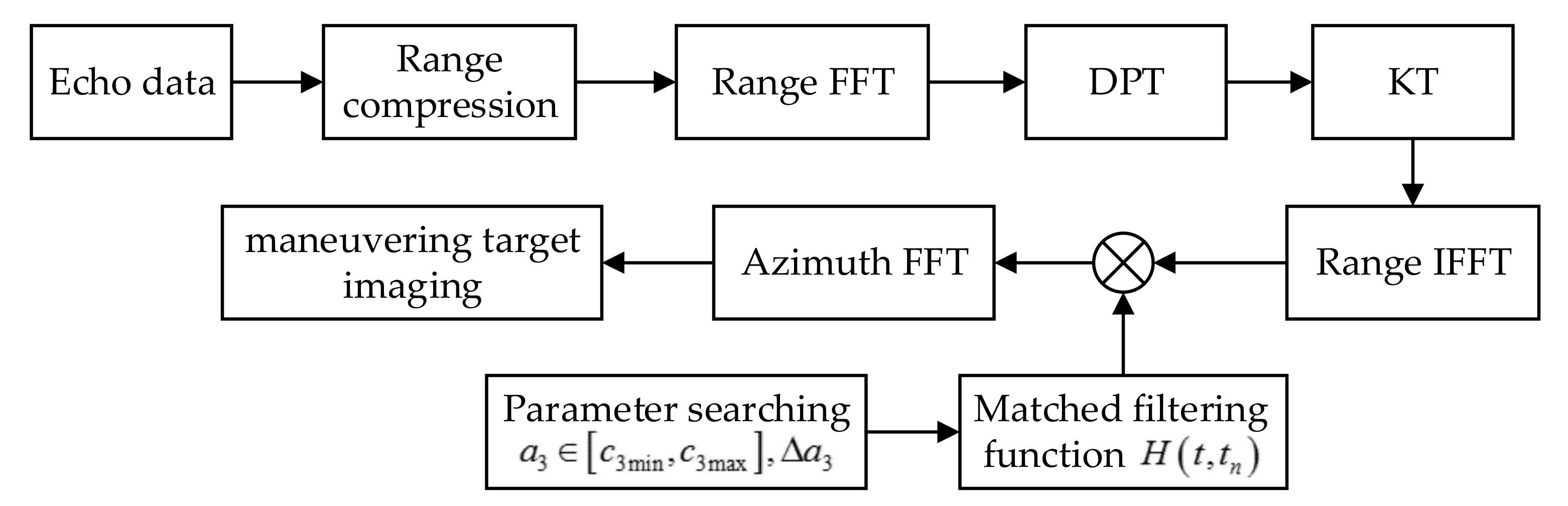
3. Algorithm Description

3.1. DPT–KT–MFP Algorithm with Single Target

The DPT [38,39] can be applied to decrease the target phase order, which can be stated as

$$s_2\left(f,t_m\right)=s_1\left(f,t_m+\frac{{\tau }_0}{2}\right)\cdot {\left[s_1\left(f,t_m-\frac{{\tau }_0}{2}\right)\right]}^{\ast },$$

(7)

where $\ast$ is the conjugate operation, and ${\tau }_0$ is the fixed delay time, which is usually very small. Substituting Equation (6) into Equation (7) yields

$$\begin{array}{ll}{s}_2\left(f,t_m\right)& =A_2^2\mathrm{rect}\left(\frac{f}{B}\right)w_a\left(t_m\right)\exp \left(-j\frac{4\pi n_{am}{v}_a{\tau }_0}{\lambda }\frac{f}{f_c}\right)\\ & \times \exp \left(-j\frac{\pi \left(4v_{base}{\tau }_0+c_3{\tau }_0^3\right)}{\lambda }\left(\frac{f+f_c}{f_c}\right)\right)\exp \left(-j\frac{4\pi \left(2c_2{\tau }_0{t}_m+3c_3{\tau }_0{t}_m^2\right)}{\lambda }\left(\frac{f+f_c}{f_c}\right)\right).\end{array}$$

(8)

From Equation (8), we can find that the order of $t_m$ is reduced to second order, which means that the quadratic DFM and cubic RM caused by the third-order coefficient $c_3$ is removed. Moreover, under the condition of $\left(v-v_a\right)T_a\ll R_0$, the quadratic RM caused by $c_3$ can be ignored since its maximum offset $3c_3{\tau }_0{T}_a^2/4$ is much smaller than a range resolution cell. Moreover, the Doppler center and Doppler spectrum bandwidth are changed to $4c_2{\tau }_0/\lambda$ and $12c_3{\tau }_0{T}_a/\lambda$, respectively. For a ground moving target, $c_2$, $c_3$, and ${\tau }_0$ are so small that the azimuth Doppler spectrum of the maneuvering target is entirely distributed in the non-ambiguous Doppler area. Thus, the problem of Doppler center blur and Doppler spectrum ambiguity is effectively addressed. However, the linear RM caused by $c_2$ and linear DFM induced by $c_3$ still exist after the DPT procedure, which can deteriorate the focusing performance.

In [14,24,39], several algorithms were proposed to correct the RM related to second-order coefficient $c_2$ by constructing a compensation function. However, constructing the compensation function needs some prior knowledge, such as platform velocity or the target’s nearest slant range, which cannot always be accurately obtained. Additionally, the compensation error of RM caused by these methods [14,24,39] may be larger than a range resolution cell in the high-resolution case, which may result in a serious refocusing performance loss.

Consequently, in this paper, the KT was applied to absolutely remove the linear RM without any prior knowledge. The KT can be stated as follows [10,11,12,13,14,24,29]:

$$t_m=\frac{f_c}{f+f_c}{t}_n,$$

(9)

where $t_n$ indicates the new slow-time variable. Substituting Equation (9) into Equation (8) yields

$$\begin{array}{l}{s}_2\left(f,t_n\right)=A_2^2\mathrm{rect}\left(\frac{f}{B}\right)w_a\left(t_n\right)\exp \left(-j\frac{4\pi n_{am}{v}_a{\tau }_0}{\lambda }\frac{f}{f_c}\right)\exp \left(-j\frac{8\pi c_2{\tau }_0{t}_n}{\lambda }\right)\\ \begin{array}{cc}\begin{array}{cc}& \end{array}& \end{array}\times \exp \left(-j\frac{12\pi c_3{\tau }_0{t}_n^2}{\lambda }\left(\frac{f_c}{f+f_c}\right)\right)\exp \left(-j\frac{\pi \left(4v_{base}{\tau }_0+c_3{\tau }_0^3\right)}{\lambda }\left(\frac{f+f_c}{f_c}\right)\right).\end{array}$$

(10)

Under the narrowband condition, $f_c/\left(f+f\right)\approx 1-f/f_c$, Equation (10) can be rewritten as

$$\begin{array}{l}{s}_2\left(f,t_n\right)=A_2^2\mathrm{rect}\left(\frac{f}{B}\right)w_a\left(t_n\right)\exp \left(-j\frac{4\pi n_{am}{v}_a{\tau }_0}{\lambda }\frac{f}{f_c}\right)\exp \left(-j\frac{8\pi c_2{\tau }_0{t}_n}{\lambda }\right)\\ \begin{array}{cc}\begin{array}{cc}& \end{array}& \end{array}\times \exp \left(-j\frac{12\pi c_3{\tau }_0{t}_n^2}{\lambda }\left(1-\frac{f}{f_c}\right)\right)\exp \left(-j\frac{\pi \left(4v_{base}{\tau }_0+c_3{\tau }_0^3\right)}{\lambda }\left(\frac{f+f_c}{f_c}\right)\right).\end{array}$$

(11)

From Equation (11), one can see that the coupling between the $t_n-\mathrm{term}$ and $f$ is removed, which means that the linear RM is effectively corrected. Moreover, as for the ground maneuvering target, the $\exp \left(-j12\pi c_3{\tau }_0{t}_n^{2}f/c\right)$ can be ignored because its value is much smaller than $\pi /4$ due to the small values of $c_3$ and ${\tau }_0$ [27].

After performing the range IFFT on Equation (11), we obtain

$$\begin{array}{l}{s}_3\left(t,t_n\right)=A_3{w}_a\left(t_n\right)\sin \mathrm{c}\left\{t-\frac{2c_1{\tau }_0}{c}-\frac{c_3{\tau }_0^3}{2c}\right\}\exp \left(-j\frac{8\pi c_2{\tau }_0{t}_n}{\lambda }\right)\\ \begin{array}{cc}\begin{array}{cc}& \end{array}& \end{array}\times \exp \left(-j\frac{12\pi c_3{\tau }_0{t}_n^2}{\lambda }\right)\exp \left(-j\frac{\pi }{\lambda }\left(4v_{base}{\tau }_0+c_3{\tau }_0^3\right)\right),\end{array}$$

(12)

where $A_3$ represents the echo amplitude after IFFT. From Equation (12), we can find that the RM containing linear, quadratic, and cubic RM is effectively removed via the previous operation. However, due to the existence of the linear DFM caused by third-order coefficient $c_3$, the maneuvering target is still seriously defocused if we directly apply the azimuth FFT to accumulate the target energy. The previous methods proposed in [24,31,33,39] assumed that the target signal is an LFM signal after correcting the RM, and they utilized time–frequency analysis algorithms to remove the linear DFM. Nevertheless, these methods need to search the range cells for extracting the target energy, which greatly increases the computational complexity. Actually, the maximum offset of linear DFM induced by $c_3$, which is equal to $12c_3{\tau }_0{T}_a/\lambda$, is usually very small because of the small values of $c_3$ and ${\tau }_0$. The linear DFM induced by $c_3$ only spans across several Doppler frequency resolution cells. Therefore, the searching third-order coefficient is much smaller than the searching range cells. Hence, we constructed a matched filtering function to remove the linear DFM, which can be expressed as

$$H\left(t,t_n\right)=\exp \left(j\frac{12\pi a_3{\tau }_0{t}_n^2}{\lambda }\right),$$

(13)

where $a_3=l\Delta a_3\left(l=-L/2,\dots ,L/2-1\right)$ is the searching third-order coefficient, $L$ denotes the size of the searching third-order coefficient, and $\Delta a_3$ is the searching step of $a_3$.

From Equation (14), we can find that the Doppler frequency related to $a_3$ is $12a_3{\tau }_0{t}_n/\lambda$. The criterion for selecting $\Delta a_3$ is that the maximum offset of $12\Delta a_3{\tau }_0{t}_n/\lambda$ is equal to a Doppler frequency resolution cell in one coherent process interval [23]. Therefore, the $\Delta a_3$ can be described as

$$\Delta a_3=\frac{\lambda f_{prf}^2}{12M^2{\tau }_0}.$$

(14)

When $a_3$ is equal to $c_3$, multiplying Equation (13) by Equation (12) and performing the azimuth FFT yields

$$\begin{array}{l}{s}_4\left(t,f_n\right)={\mathrm{FFT}}_{t_n}\left[s_3\left(t,t_n\right)\times H\left(t,t_n\right)\right]=A_4\sin \mathrm{c}\left\{t-\frac{2c_1{\tau }_0}{c}-\frac{c_3{\tau }_0^3}{2c}\right\}\\ \begin{array}{cc}& \begin{array}{cc}& \end{array}\end{array}\times \sin \mathrm{c}\left(f_n+\frac{4c_2{\tau }_0}{\lambda }\right)\exp \left(-j\frac{4\pi v_{base}{\tau }_0}{\lambda }\right)\exp \left(-j\frac{\pi c_3{\tau }_0^3}{\lambda }\right),\end{array}$$

(15)

where ${\mathrm{FFT}}_{t_n}\left[\right]$ denotes the FFT operation, $A_4$ is the signal amplitude after FFT operation, and $f_n$ indicates the Doppler frequency variable corresponding to $t_n$. From Equations (13) and (15), it can be seen that, when the third-order coefficient $c_3$ is matched exactly, the maneuvering target is well refocused at $t=2c_1{\tau }_0/c+0.5c_3{\tau }_0^3/c$ and $f_n=-4c_2{\tau }_0/\lambda$. As a result, using the peak detection technique [40], $c_1$, $c_2$, and $c_3$ can be estimated as follows:

$${\widehat{c}}_3=\underset{a_3}{\arg \max }\left|{\mathrm{FFT}}_{t_n}\left\{{\mathrm{IFFT}}_f\left[\mathrm{KT}\left[\mathrm{DPT}\left(s_1\left(f,t_m\right)\right)\right]\right]\times H\left(t,t_n\right)\right\}\right|,$$

(16)

$${\widehat{c}}_1=\frac{2c\widehat{t}-{\widehat{c}}_3{\tau }_0^3}{4{\tau }_0}\begin{array}{cc}\begin{array}{cc}& \end{array}& \end{array}{\widehat{c}}_2=-\frac{{\widehat{f}}_n\lambda }{4{\tau }_0}.$$

(17)

According to the aforementioned analyses, we know that the presented algorithm can effectively remove the effects of Doppler center blur, Doppler spectrum ambiguity, high-order RM, and DFM, as well as refocus the maneuvering target. Figure 3 gives the flowchart of the presented method.

Below, we give an example to demonstrate that the presented algorithm can effectively refocus a ground maneuvering target.

Example 1: Suppose a ground maneuvering target exists in the observation area. The radar system parameters are listed in

Table 1. System parameters of radar.

Parameter	Value
Carrier frequency	6 GHZ
Range bandwidth	200 MHZ
Range sampling frequency	300 MHZ
Pulse repetition frequency	800 HZ
Pulse width	1 µs
Synthetic aperture time	2 s
Platform velocity	250 m/s

, and the motion parameters of maneuvering target are set as follows: the nearest slant range $R_0=3000$ m, the along-track velocity $v_a=23$ m/s, the along-track acceleration $a_a=-4.5$ m/s², the cross-track velocity $v_c=32$ m/s, and the cross-track acceleration $a_c=-3.6$ m/s². According to Equation (1), the first-, second-, and third-order coefficients can be calculated as $c_1=-32$ m/s, $c_2=10.3882$ m/s², and $c_3=0.2619$ m/s³. The simulation results are given in Figure 4.

Figure 4a gives the range compression result. Obviously, serious RM containing linear, quadratic, and cubic RM occurs. The target Doppler spectrum is given in Figure 4b. It can be seen that the target spectrum occupies three PRF bands, as shown in Figure 2c, which means that serious Doppler spectrum ambiguity appears. The target trajectory after DPT operation is shown in Figure 4c, from which we can find that an oblique straight line is present, which means that the quadratic and cubic RM is effectively removed. The target spectrum after DPT operation is given in Figure 4d. We can observe that the target spectrum is overall distributed in one PRF band, which means that the problem of Doppler spectrum ambiguity is addressed. Additionally, the Doppler center blur is also eliminated after DPT operation, since the Doppler center is changed from $320$ H_Z ($n_{am}=-2$) to $166.2$ H_Z ($n_{am}=0$). Figure 4e shows the result after KT operation. We can find that target trajectory becomes one straight line along the slow-time axis, which means that the residual linear RM is effectively corrected. Figure 4f shows the searching result of the third-order coefficient. Obviously, according to the peak position, $c_3$ can be estimated as $0.2624$ m/s³. After correcting the linear DFM using the estimated third-order coefficient, we can observe that a distinct peak appears in Figure 4g, which indicates that the presented algorithm can effectively remove the Doppler center blur, Doppler spectrum ambiguity, high-order RM, and DFM, as well as refocus the maneuvering target. On the basis of peak detection technology [40], the first- and second-order coefficients can be estimated as follows: ${\widehat{c}}_1=32.0013$ m/s and ${\widehat{c}}_2=10.3875$ m/s².

3.2. DPT–KT–MFP Algorithm with Multiple Targets

With respect to refocusing multiple maneuvering targets, cross-term interference is inevitably introduced because of the existence of nonlinear transform in our proposed method. In this subsection, the effects of cross-terms are analyzed. Suppose that $K$ maneuvering targets exist in the observation area; then, the range compression signal in $f-t_m$ domain can be stated as

$$\begin{array}{l}{s}_{mul,1}\left(f,t_m\right)={\displaystyle \sum _{i=1}^K{A}_{2,i}\mathrm{rect}\left(\frac{f}{B}\right)w_a\left(t_m\right)}\exp \left[-j\frac{4\pi R_{0,i}}{c}\left(f+f_c\right)\right]\\ \times \exp \left(-j\frac{4\pi f}{c}{n}_{am,i}{v}_a{t}_m\right)\exp \left[-j\frac{4\pi }{c}\left(f+f_c\right)\left(v_{base,i}{t}_m+c_{2,i}{t}_m^2+c_{3,i}{t}_m^3\right)\right],\end{array}$$

(18)

where $A_{2,i}$ represents the $i\mathrm{th}$ target’s amplitude, and $R_{0,i}$ denotes the $i\mathrm{th}$ target’s nearest slant range. $n_{am,i}$, $v_{base,i}$, $c_{2,i}$, and $c_{3,i}$ represent the Doppler ambiguity number, baseband velocity, second- and third-order coefficients of the $i\mathrm{th}$ moving target, respectively.

After performing the DPT, we obtain

$$\begin{array}{l}{s}_{mul,1}\left(f,t_m\right)={\displaystyle \sum _{i=1}^K{A}_{2,i}^2\mathrm{rect}\left(\frac{f}{B}\right)w_a\left(t_m\right)\exp \left[-j\frac{\pi \left(4v_{0,i}{\tau }_0+c_{3,i}{\tau }_0^3\right)}{\lambda }\left(\frac{f+f_c}{f_c}\right)\right]}\\ \times \exp \left[-j\frac{4\pi \left(2c_{2,i}{t}_m+3c_{3,i}{t}_m^2\right){\tau }_0}{\lambda }\left(\frac{f+f_c}{f_c}\right)\right]\exp \left(-j\frac{4\pi n_{am,i}{v}_a{\tau }_0}{\lambda }\frac{f}{f_c}\right)+R_{\mathrm{c}ross}\left(f,t_m\right),\end{array}$$

(19)

where

$$\begin{array}{cc}\hfill & R_{cross}\left(f,t_m\right)=\sum _{i=1}^K\sum _{j=1,i\ne j}^K{A}_{2,i}{A}_{2,j}\mathrm{rect}\left(\frac{f}{B}\right)w_a\left(t_m\right)exp\left[-j\frac{4\pi }{\lambda }\left(\frac{f+f_c}{f_c}\right)\left(R_{0,i}-R_{0,j}\right)\right]\hfill \\ \hfill & \times exp\left[-j\frac{4\pi v_a{t}_m}{\lambda }\frac{f}{f_c}\left(n_{am,i}-n_{am,j}\right)\right]exp\left[-j\frac{2\pi v_a{\tau }_0}{\lambda }\frac{f}{f_c}\left(n_{am,i}+n_{am,j}\right)\right]\hfill \\ \hfill & \times exp\left[-j\frac{4\pi }{\lambda }\left(\frac{f+f_c}{f_c}\right)\left(v_{0,i}-v_{0,j}\right)t_m\right]exp\left[-j\frac{2\pi }{\lambda }\left(\frac{f+f_c}{f_c}\right)\left(v_{0,i}+v_{0,j}\right){\tau }_0\right]\hfill \\ \hfill & \times exp\left[-j\frac{\pi }{\lambda }\left(\frac{f+f_c}{f_c}\right)\left(c_{2,i}-c_{2,j}\right)\left(4t_m^2+{\tau }_0^2\right)\right]exp\left(-j\frac{4\pi }{\lambda }\left(\frac{f+f_c}{f_c}\right)\left(c_{2,i}+c_{2,j}\right)t_m{\tau }_0\right)\hfill \\ \hfill & \times exp\left[-j\frac{\pi }{\lambda }\left(\frac{f+f_c}{f_c}\right)\left(c_{3,i}-c_{3,j}\right)\left(4t_m^3+3t_m{\tau }_0^2\right)\right]exp\left[-j\frac{\pi }{\lambda }\left(\frac{f+f_c}{f_c}\right)\left(c_{3,i}+c_{3,j}\right)\left(6t_m^2{\tau }_0+0.5{\tau }_0^3\right)\right].\hfill \end{array}$$

(20)

From Equations (19) and (20), it can be seen that, with respect to the auto-terms after DPT, the cubic RM and quadratic DFM are effectively removed. Furthermore, similar to refocusing the single target, the quadratic RM caused by $c_{3,i}$ can be ignored since its maximum offset $3c_{3,i}{\tau }_0{T}_a^2/4$ is much smaller than a range resolution cell. For the cross-terms after DPT, the high-order RM and DFM are still present, because the $t_m-\mathrm{term}$, $t_m^2-\mathrm{term}$, and $t_m^3-\mathrm{term}$ are still coupled with $f$. Consequently, after carrying out the KT and MFP operations as described in Section 3.1, the energy of the auto-terms is well coherently accumulated, while the energy of the cross-terms cannot be integrated effectively because of the high-order RM and DFM. In addition, the proposed method can also refocus the maneuvering targets in the case of close multiple targets, since the $R_{0,i}$ in auto-terms is effectively removed after DPT operation. On the basis of the aforementioned analyses, we can conclude that the presented method is able to remove the effects of cross-terms and refocus the ground maneuvering targets in the case of multiple targets. Next, several simulation experiments are presented to validate how the presented method suppresses the cross-terms and focuses the auto-terms.

Example 2: Assume two maneuvering targets, represented by T1 and T2, exist in the observation area. The radar system parameters are the same as those in Example 1. In addition, the motion parameters of the two maneuvering targets are set as follows: $R_{0,1}=2940 \mathrm{m}$, $v_{a,1}=11 \mathrm{m}/\mathrm{s}$, $a_{a,1}=-4.5 {\mathrm{m}/\mathrm{s}}^2$, $v_{c,1}=32 \mathrm{m}/\mathrm{s}$, and $a_{c,1}=-3.6 {\mathrm{m}/\mathrm{s}}^2$ for T1; $R_{0,2}=3050 \mathrm{m}$, $v_{a,2}=13 \mathrm{m}/\mathrm{s}$, $a_{a,2}=4.3 {\mathrm{m}/\mathrm{s}}^2$, $v_{c,2}=-36 \mathrm{m}/\mathrm{s}$, and $a_{c,2}=-1.5 {\mathrm{m}/\mathrm{s}}^2$ for T2. On the basis of Equation (1), the first-, second-, and third-order coefficients of T1 and T2 can be calculated as follows: $c_{1,1}=-32$, $c_{2,1}=11.5145$, and $c_{3,1}=0.2886$ for T1; $c_{1,2}=36$, $c_{2,2}=9.9580$, and $c_{3,2}=-0.2758$ for T2. Figure 5 gives the simulation results.

Figure 5a gives the target trajectories after range compression. Obviously, the targets’ energy spans across several range cells during the coherent integration time. After DPT and KT operations, the RM correction result is given in Figure 5b, from which it can be seen that the energy of T1 and T2 is concentrated in the same range cells, while the energy of cross-terms still spans across several range cells. Figure 5c shows the searching result of the third-order coefficient. It can be seen that two distinct peaks exist. According to the peak positions, the third-order coefficients of T1 and T2 can be estimated as follows: ${\widehat{c}}_{3,1}=0.2879$ and ${\widehat{c}}_{3,2}=-0.2778$. After compensating for the linear DFM using the estimated third-order coefficients, Figure 5d,e give the final focusing results of T1 and T2, respectively. Obviously, two well-focused peaks appear in Figure 5d,e, which demonstrates that the propose algorithm can effectively eliminate the effects of cross-terms and integrate the energy of auto-terms. According to the peak position, the remaining motion parameters of T1 and T2 can be estimated as follows: ${\widehat{c}}_{1,1}=-31.9975$ and ${\widehat{c}}_{2,1}=11.5162$ for T1; ${\widehat{c}}_{1,2}=36.0019$ and ${\widehat{c}}_{2,2}=9.9589$ for T2.

3.3. Computational Complexity Analysis

Next, the computational cost of GRFT [28], SOKT–GHHAF [31], TRT–SOKT–LVD [33], and the proposed method was analyzed. Suppose $N$, $M$, and $M_{\tau }$ represent the numbers of range cells, echo pulses, and lag samples, respectively, and the number of searching first-, second-, and third-order coefficients is the same, denoted as $N_1$. The computational complexity of GRFT based on 4D brute-force search is approximately $\mathrm{O}\left(N_1^{3}NM\right)$. The procedures of the SOKT–GHHAF mainly include a SOKT operation, whose computational complexity is approximately $NM\mathrm{O}\left({\log }_{2}M\right)$, a Hough transform (HT) operation, with a computational cost of $\mathrm{O}\left(N{M}^2\right)$, a GHHAF operation, whose computational complexity is approximately $\mathrm{O}\left(3M^2+M^3+N_{1}M{\log }_{2}M\right)$, and a range cell search operation. Consequently, the total computational cost of SOKT–GHHAF is approximately $NM\mathrm{O}\left({\log }_{2}M\right)+\mathrm{O}\left(N{M}^2\right)+N\mathrm{O}\left(3M^2+M^3+N_{1}M{\log }_{2}M\right)$. The procedures of the TRT–SOKT–LVD mainly include a TRT operation, whose computational cost is approximately $\mathrm{O}\left(NM\right)$, an SOKT operation with a computational complexity of $NM\mathrm{O}\left({\log }_{2}M\right)$, an LVD operation, whose computational complexity is approximately $M{M}_{\tau }\mathrm{O}\left(5{\log }_{2}M+{\log }_2{M}_{\tau }\right)$, and a range cell search operation. As a consequence, the total computational cost of TRT–SOKT–LVD is approximately $\mathrm{O}\left(NM\right)+NM\mathrm{O}\left({\log }_{2}M\right)+NM{M}_{\tau }\mathrm{O}\left(5{\log }_{2}M+{\log }_2{M}_{\tau }\right)$. In addition, the procedures of the proposed algorithm mainly include a DPT operation with a computational cost of $\mathrm{O}\left(NM\right)$, a KT operation with a computational complexity of $NM\mathrm{O}\left({\log }_{2}M\right)$, and an MFP operation, whose computational cost is approximately $N_{1}NM\mathrm{O}\left({\log }_{2}M\right)$. Therefore, the total computational cost of the proposed method is approximately $\mathrm{O}\left(NM\right)+\left(NM+N_{1}NM\right)\mathrm{O}\left({\log }_{2}M\right)$. The computational complexity of the abovementioned four algorithms is listed in

Table 2. Comparison of computational complexity. GRFT, generalized radon Fourier transform; SOKT–GHHAF, second-order KT and Hough-generalized high-order ambiguity function; TRT–SOKT–LVD, time reversing transform, second-order KT, and Lv distribution.

Methods	Computational Complexity
GRFT	$\mathrm{O}\left(N_1^{3}NM\right)$
SOKT–GHHAF	$NM\mathrm{O}\left({\log }_{2}M\right)+\mathrm{O}\left(N{M}^2\right)+N\mathrm{O}\left(3M^2+M^3+N_{1}M{\log }_{2}M\right)$
TRT–SOKT–LVD	$\mathrm{O}\left(NM\right)+NM\mathrm{O}\left({\log }_{2}M\right)+NM{M}_{\tau }\mathrm{O}\left(5{\log }_{2}M+{\log }_2{M}_{\tau }\right)$
Proposed	$\mathrm{O}\left(NM\right)+\left(NM+N_{1}NM\right)\mathrm{O}\left({\log }_{2}M\right)$

.

Assume $N=M=M_{\tau }=N_1$; then, the computational costs of GRFT, SOKT–GHHAF, TRT–SOKT–LVD, and the presented method are approximately $\mathrm{O}\left(N^5\right)$, $\mathrm{O}\left(N^4\right)$, $\mathrm{O}\left(N^3{\log }_{2}N\right)$, and $\mathrm{O}\left(N^3{\log }_{2}N\right)$, respectively. Obviously, compared with GRFT and SOKT–GHHAF, the presented method has a much lower computational burden. Compared with the TRT–SOKT–LVD, the proposed algorithm has a similar computational burden under the above-assumed condition. Actually, with respect to the ground maneuvering target, the number of searching range cells $N$ is usually far greater than the number of searching third-order coefficients $N_1$. Consequently, the presented algorithm has a higher computational efficiency than the TRT–SOKT–LVD algorithm.

Below, the computational time of these four methods is compared, where the target’s motion parameters and radar parameters are the same as those in Example 1 (the processor of the computer was a Intel (R) Core (TM) i7-4790 central processing unit (CPU) @3.60 GHz; the random-access memory (RAM) was 8 GB; the software was MATLAB 2014a).

Table 3. Comparison of computational time.

Methods	Computational Time (s)
GRFT	3382
SOKT–GHHAF	279.2
TRT–SOKT–LVD	36.5
Proposed	3.49

shows the computational time of these methods, from which it can be seen that the presented algorithm is more efficient in comparison with the other three algorithms.

4. Simulation and Real Data Processing Results

4.1. Analysis and Discussion of Simulation Results

In this subsection, we adopt a simulated ideal point target to validate the effectiveness of the presented DPT–KT–MFP algorithm under the Gaussian noise environment. The target’s motion parameters and radar parameters are the same as those in Example 1. In order to better show the superior performance of the presented DPT–KT–MFP algorithm, GRFT [28], SOKT–GHHAF [31], TRT–SOKT–LVD [33], and moving target detection (MTD) are performed for comparison.

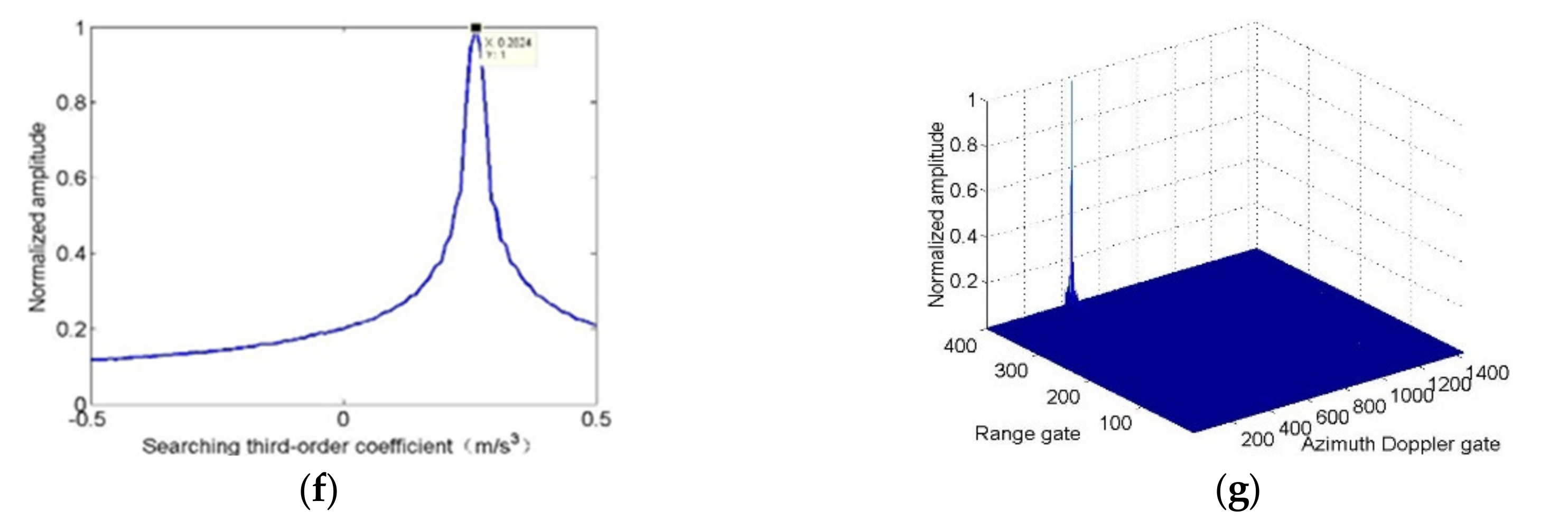
4.1.1. Maneuvering Target Integration Performance

In Figure 6, we first evaluate the integration performance of the presented algorithm for a maneuvering target. The signal-to-noise ratio (SNR) after range compression was set as 6 dB. It is worth noting that, on the basis of the target’s motion parameters and radar system parameters set above, Doppler ambiguity (containing Doppler center blur and Doppler spectrum ambiguity) occurs. The target trajectory after range compression is shown in Figure 6a, from which we can find that the target energy is distributed in multiple range cells. Figure 6b gives the direct KT result. One can see that the trajectory of the maneuvering target is split into three parts since its Doppler spectrum occupies three PRF bands. Figure 6c gives the result after DPT and KT, from which noise is removed to clearly show the target trajectory. We can observe that the target energy is distributed in one range cell, since the RM, Doppler center blur, and Doppler spectrum ambiguity are eliminated after DPT and KT operations. The refocusing result of the presented DPT–KT–MFP algorithm is given in Figure 6d. It can be seen that the target energy is well coherently integrated as a distinct peak. Figure 6e gives the MTD result. One can see that the MTD method cannot effectively accumulate the target energy because of the high-order RM and DFM caused by the complex motions of the maneuvering target. Figure 6f gives the focusing result of SOKT–GHHAF. Obviously, the SOKT–GHHAF method is invalid because of the Doppler spectrum ambiguity and the application of the incoherent integration algorithm. The result after TRT and SOKT is shown in Figure 6g. Similar to Figure 6c, the noise is removed to clearly show the target trajectory. We can observe that the target trajectory splits into five parts since the bandwidth of the target Doppler spectrum is doubled after TRT. Therefore, only a small fraction of target energy is accumulated by TRT–SOKT–LVD. Figure 6h gives the TRT–SOKT–LVD result. Obviously, the maneuvering target is still seriously defocused due to the effects of Doppler spectrum ambiguity. The GRFT result is shown in Figure 6i. We can observe that the integration performance of the GRFT algorithm is better than the presented algorithm. Nevertheless, the good accumulation performance is at the cost of a high computational burden.

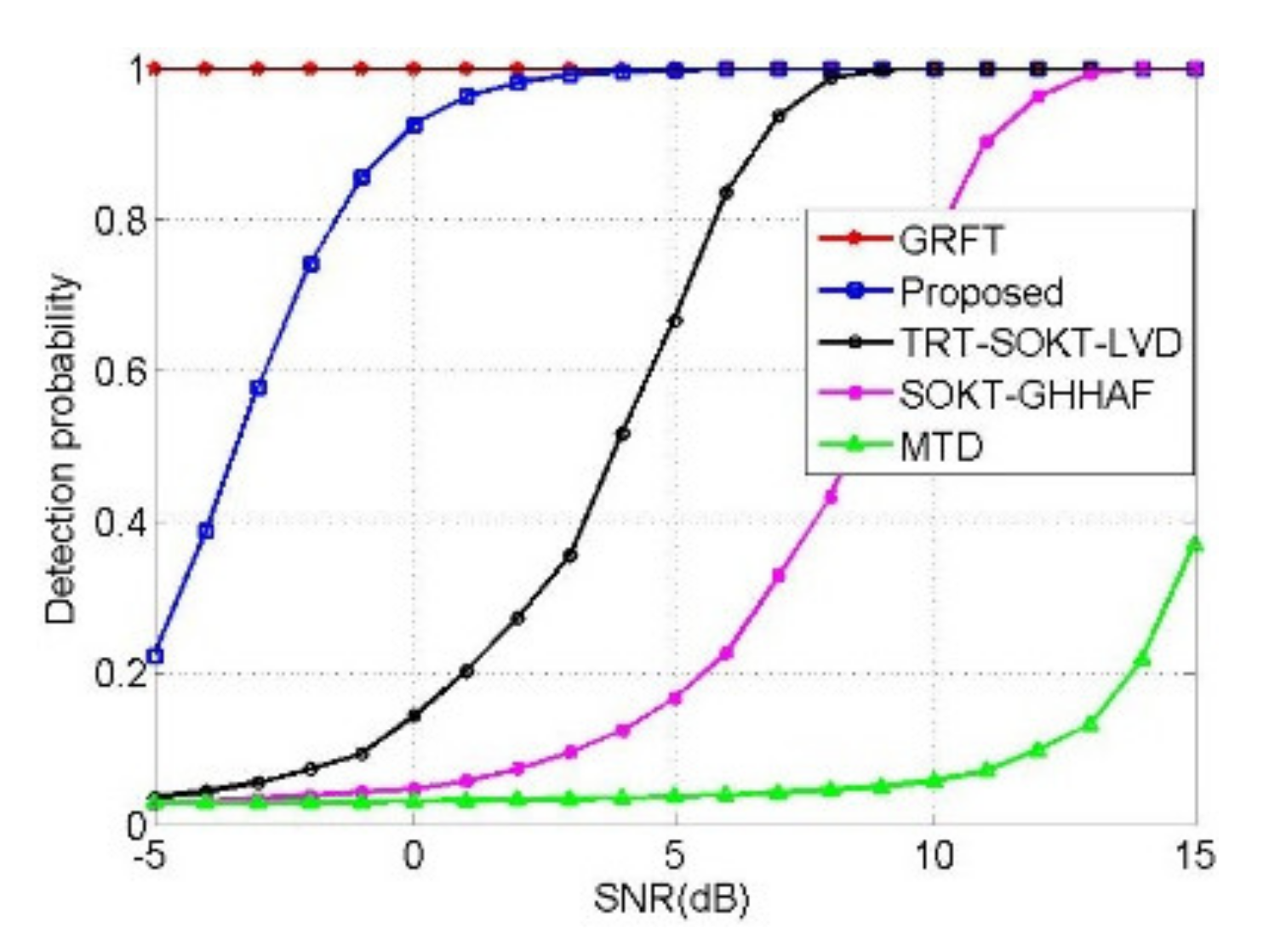
4.1.2. Maneuvering Target Detection Ability

Below, we analyze the detection ability of MTD, SOKT–GHHAF, TRT–SOKT–LVD, GRFT, and the proposed method via Monte Carlo trials. The constant false alarm probability was set at ${10}^{-6}$. After performing 500 Monte Carlo trials at every input SNR, Figure 7 shows the curves of detection probability varying with range compression SNRs. Obviously, the target detection performance of the presented algorithm was superior to that of the MTD, SOKT–GHHAF, and TRT–SOKT–LVD methods, since the effects of high-order RM and DFM, Doppler center blur, and Doppler spectrum ambiguity are effectively eliminated by the proposed algorithm. Compared with the GRFT method, the presented algorithm has a similar target detection ability but with a much lower computational cost when the input SNR is larger than $0\mathrm{dB}$. Unfortunately, the proposed method may suffer from a great detection performance loss in cases with low SNR, since the DPT is a nonlinear transform.

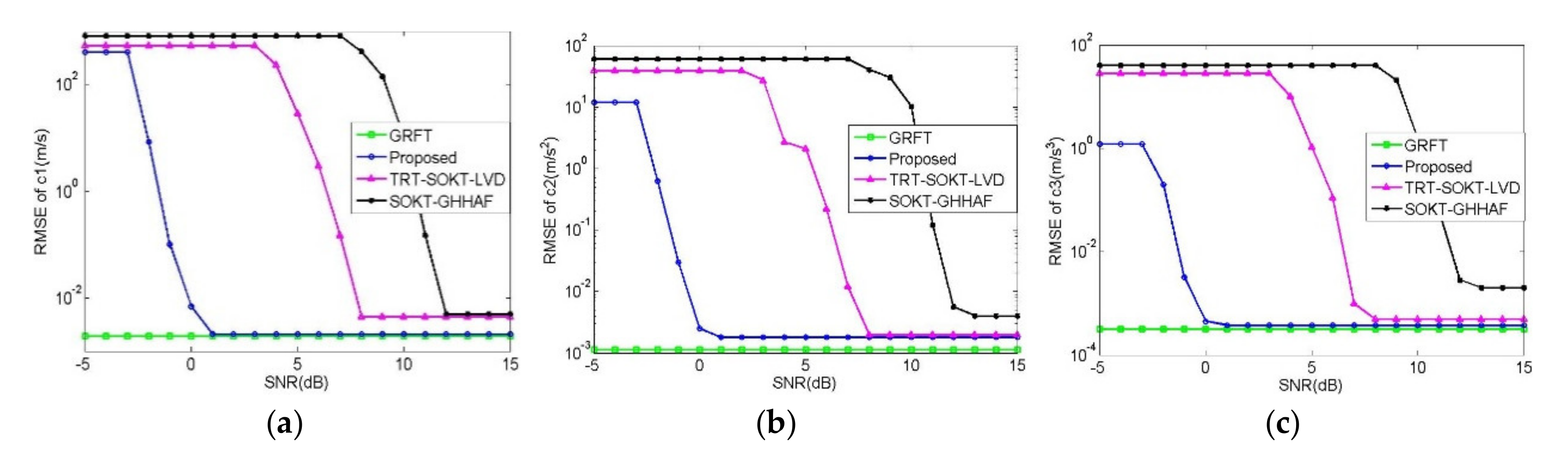
4.1.3. Motion Parameter Estimation Performance

Next, the motion parameter estimation performance of SOKT–GHHAF, TRT–SOKT–LVD, GRFT, and the presented algorithm was also compared via Monte Carlo trials, in which the input range-compressed SNRs varied from $-15 \mathrm{dB}$ to $5 \mathrm{dB}$ with a step size of 1 dB. Moreover, at every input SNR, we carry out 500 Monte Carlo trials. Figure 8a–c show the root-mean-square errors (RMSEs) of the estimated first-, second-, and third-order coefficients varying with input SNRs, respectively. From Figure 8, one can see that the motion parameter estimation performance of SOKT–GHHAF method deteriorates severely, since the effects of Doppler ambiguity and cubic RM are ignored, and the HT, which is the incoherent integration operation, is used twice in the SOKT–GHHAF method. Moreover, SOKT–GHHAF has a huge computational burden due to the application of three 1D parameter searches. The TRT–SOKT–LVD method suffers from a great performance loss of parameter estimation, because it cannot remove the Doppler spectrum ambiguity. In comparison with the other three algorithms, the GRFT method can acquire the optimal motion parameter estimation performance, but it needs a 4D parameter search, which makes it difficult to implement in practice. When the input SNR is larger than $0\mathrm{dB}$, the motion parameter estimation performance of the presented algorithm is similar to that of the GRFT algorithm. Moreover, compared with the GRFT algorithm, the presented algorithm has a higher computational efficiency, since it only needs to search the third-order coefficient, whose value is usually very small for ground maneuvering targets.

4.2. Analysis and Discussion of Real Data Processing Results

In this subsection, we verify the effectiveness of the presented refocusing algorithm using real radar data recorded by an X-band airborne radar with a broadside mode. This radar has three apertures in the along-track direction, whereby one aperture transmits the signals and all three apertures receive the reflected echoes. The observed targets were cooperative moving trucks driving along the road. The SAR system parameters are listed in

Table 4. X-band SAR system parameters.

Parameter	Value
Carrier frequency	$8.85 \mathrm{GHz}$
Range bandwidth	$40 \mathrm{MHz}$
Range sampling frequency	$60 \mathrm{MHz}$
Pulse repetition frequency	$1000 \mathrm{Hz}$
Pulse width	10 µs
Platform velocity	$120 \mathrm{m}/\mathrm{s}$
Swath central range	$9000 \mathrm{m}$

.

Figure 9a gives the image of the ground maneuvering targets. We can observe that the maneuvering targets are submerged by strong ground clutter. In order to obtain a higher target signal-to-clutter-plus-noise-ratio (SCNR), we carried out the extended factored algorithm [41] to suppress the ground clutter. After clutter suppression, Figure 9b shows that several clear targets appear. However, the maneuvering targets are seriously smeared because of the RM and DFM. Below, we utilize a maneuvering target of interest marked by a red ellipse to demonstrate the effectiveness of the presented algorithm. The range compression result of the interested target is given in Figure 9c, from which we can find that the interested target energy is distributed in multiple range cells because of severe RM. The target trajectory after DPT and KT is shown in Figure 9d. it can be seen that the trajectory of the maneuvering target is parallel to the slow-time axis, which means that the RM is effectively eliminated. Figure 9e gives the focusing result of the presented algorithm. We can observe that a well-refocused peak appears since the high-order RM and DFM are absolutely removed, which proves the effectiveness of the presented DPT–KT–MFP algorithm.

5. Conclusions

In this paper, the DPT–KT–MFP algorithm was presented to address the refocusing and motion parameter estimation problems for ground maneuvering targets, involving Doppler ambiguity, high-order RM, and DFM during the coherent integration time. Obviously, the proposed algorithm can effectively remove the high-order RM and DFM induced by complex motions of ground maneuvering targets, as well as realize the target refocusing with low computational complexity. In addition, the Doppler ambiguity containing Doppler center blur and Doppler spectrum ambiguity can also be effectively dealt with due to the DPT operation. Furthermore, for refocusing of multiple targets, the presented algorithm is able to eliminate the effects of cross-terms in which high-order RM and DFM still exist. Compared with conventional algorithms which ignore the effects of Doppler ambiguity and the target’s high-order motions, the presented algorithm can acquire better focusing performance and motion parameter estimation precision. Furthermore, compared with the GRFT method, the presented algorithm has higher computational efficiency and similar focusing performance in the case of a high SNR.

References

1. Zhu, S.; Liao, G.; Qu, Y.; Zhou, Z.; Liu, X. Ground moving targets imaging algorithm for synthetic aperture radar. IEEE Trans. Geosci. Remote Sens. 2011, 49, 462–477. [Google Scholar] [CrossRef]
2. Bovenga, F.; Derauw, D.; Rana, F.M.; Barbier, C.; Refice, A.; Veneziani, N.; Vitulli, R. Multi-chromatic analysis of SAR images for coherent target detection. Remote Sens. 2014, 6, 8822–8843. [Google Scholar] [CrossRef] [Green Version]
3. Filippo, B. COSMO-SkyMed staring spotlight SAR data for micro-motion and inclination angle estimation of ships by pixel tracking and convex optimization. Remote Sens. 2019, 11, 766. [Google Scholar] [CrossRef] [Green Version]
4. Wan, J.; Zhou, Y.; Zhang, L.; Chen, Z. A doppler ambiguity tolerated method for radar sensor maneuvering target focusing and detection. IEEE Sens. J. 2019, 19, 6691–6704. [Google Scholar] [CrossRef]
5. Huang, Y.; Liao, G.; Xu, J.; Li, J.; Yang, D. GMTI and parameter estimation for MIMO SAR system via fast interferometry RPCA method. IEEE Trans. Geosci. Remote Sens. 2018, 56, 1774–1787. [Google Scholar] [CrossRef]
6. Zhang, X.; Liao, G.; Zhu, S.; Zeng, C.; Shu, Y. Geometry-information-aided efficient radial velocity estimation for moving target imaging and location based on Radon transform. IEEE Trans. Geosci. Remote Sens. 2015, 53, 1105–1117. [Google Scholar] [CrossRef]
7. Li, D.; Zhan, M.; Liu, H.; Liao, Y.; Liao, G. A Robust Translational Motion Compensation Method for ISAR Imaging Based on Keystone Transform and Fractional Fourier Transform Under Low SNR Environment. IEEE Trans. Aerosp. Electron. Syst. 2017, 53, 2140–2156. [Google Scholar] [CrossRef]
8. Tian, M.; Liao, G.; Zhu, S.; He, X.; Li, Y. A novel method for high-speed maneuvering target detection and motion parameters estimation. Multidimens. Syst. Signal Process. 2020, 4, 1625–1647. [Google Scholar] [CrossRef]
9. Li, D.; Ma, H.; Liu, H.; Chen, Z.; Yang, Z. An efficient ground manoeuvring target refocusing method based on principal component analysis and motion parameter estimation. Remote Sens. 2020, 12, 378. [Google Scholar] [CrossRef] [Green Version]
10. Perry, R.P.; DiPietro, R.C.; Fante, R.L. SAR imaging of moving targets. IEEE Trans. Aerosp. Electron. Syst. 1999, 35, 188–200. [Google Scholar] [CrossRef]
11. Zhu, D.; Li, Y.; Zhu, Z. A keystone transform without interpolation for SAR ground moving-target imaging. IEEE Geosci. Remote Sens. Lett. 2007, 4, 18–22. [Google Scholar] [CrossRef]
12. Li, G.; Xia, X.; Peng, Y. Doppler keystone transform: An approach suitable for parallel implementation of SAR moving target imaging. IEEE Geosci. Remote Sens. Lett. 2008, 5, 573–577. [Google Scholar] [CrossRef]
13. Sun, Z.; Li, X.; Yi, W.; Gui, G. Detection of weak maneuvering target based on keystone transform and matched filtering process. Signal Process. 2017, 140, 127–138. [Google Scholar] [CrossRef]
14. Huang, P.; Liao, G.; Yang, Z.; Xia, X.; Ma, J.; Zhang, X. An approach for refocusing of ground moving target without target motion parameter estimation. IEEE Trans. Geosci. Remote Sens. 2017, 55, 336–350. [Google Scholar] [CrossRef]
15. Rao, X.; Tao, H.; Su, J.; Guo, X.; Zhang, J. Axis rotation MTD algorithm for weak target detection. Digit. Signal Process. 2014, 26, 81–86. [Google Scholar] [CrossRef]
16. Xu, J.; Yu, J.; Peng, Y.; Xia, X. Radon–Fourier transform for radar target detection, I: Generalized Doppler filter bank. IEEE Trans. Aerosp. Electron. Syst. 2011, 47, 1186–1202. [Google Scholar] [CrossRef]
17. Xu, J.; Yu, J.; Peng, Y.; Xia, X. Radon–Fourier transform for radar target detection (II): Blind speed sidelobe suppression. IEEE Trans. Aerosp. Electron. Syst. 2011, 47, 2473–2489. [Google Scholar] [CrossRef]
18. Yu, J.; Xu, J.; Peng, Y.; Xia, X. Radon-Fourier transform for radar target detection (III): Optimality and fast implementations. IEEE Trans. Aerosp. Electron. Syst. 2012, 48, 991–1004. [Google Scholar] [CrossRef]
19. Zheng, J.; Su, T.; Liu, H.; Liao, G. Radar high-speed target detection based on the frequency-domain deramp-keystone transform. IEEE J. Sel. Top. Appl. Earth Obs. Remote Sens. 2016, 9, 285–294. [Google Scholar] [CrossRef]
20. Zhou, F.; Wu, R.; Xing, M.; Bao, Z. Approach for single channel SAR ground moving target imaging and motion parameter estimation. IET Radar Sonar Navig. 2007, 1, 59–66. [Google Scholar] [CrossRef]
21. Kirkland, D. Imaging moving targets using the second-order keystone transform. IET Radar Sonar Navig. 2011, 5, 902–910. [Google Scholar] [CrossRef]
22. Tian, J.; Cui, W.; Xia, X.; Wu, S. A novel method for parameter estimation of space moving targets. IEEE Geosci. Remote Sens. Lett. 2013, 11, 389–393. [Google Scholar] [CrossRef]
23. Chen, X.; Guan, J.; Liu, N.; He, Y. Maneuvering target detection via Radon-fractional Fourier transform-based long-time coherent integration. IEEE Trans. Signal Process. 2014, 62, 939–953. [Google Scholar] [CrossRef]
24. Huang, P.; Liao, G.; Yang, Z.; Xia, X.; Ma, J.; Zhang, X. A fast SAR imaging method for ground moving target using a second-order WVD transform. IEEE Trans. Geosci. Remote Sens. 2016, 54, 1940–1956. [Google Scholar] [CrossRef]
25. Tian, M.; Liao, G.; Zhu, S.; Liu, Y.; He, X.; Li, Y. Long-time coherent integration and motion parameters estimation of radar moving target with unknown entry/departure time based on SAF-WLVT. Digit. Signal Process. 2020, 107, 102854. [Google Scholar] [CrossRef]
26. Li, X.; Sun, Z.; Yi, W.; Cui, G.; Kong, L.; Yang, X. Computationally efficient coherent detection and parameter estimation algorithm for maneuvering target. Signal Process. 2019, 155, 130–142. [Google Scholar] [CrossRef]
27. He, X.; Liao, G.; Zhu, S.; Xu, J.; Guo, Y.; Wei, J. Fast non-searching method for ground moving target refocusing and motion parameters estimation. Digit. Signal Process. 2018, 79, 152–163. [Google Scholar] [CrossRef]
28. Xu, J.; Xia, X.; Peng, S.; Yu, J.; Peng, Y.; Qian, L. Radar maneuvering target motion estimation based on generalized Radon–Fourier transform. IEEE Trans. Signal Process. 2012, 60, 6190–6201. [Google Scholar]
29. Huang, P.; Liao, G.; Yang, Z.; Xia, X.; Ma, J. Long-time coherent integration for weak maneuvering target detection and high-order motion parameter estimation based on keystone transform. IEEE Trans. Signal Process. 2015, 64, 4013–4026. [Google Scholar] [CrossRef]
30. Kong, L.; Li, X.; Cui, G.; Yi, W.; Yang, Y. Coherent integration algorithm for a maneuvering target with high-order range migration. IEEE Trans. Signal Process. 2015, 63, 4474–4486. [Google Scholar] [CrossRef]
31. Huang, P.; Liao, G.; Yang, Z.; Xia, X.; Ma, J.; Zheng, J. Ground maneuvering target imaging and high-order motion parameter estimation based on second-order keystone and generalized Hough-HAF transform. IEEE Trans. Geosci. Remote Sens. 2017, 55, 320–335. [Google Scholar] [CrossRef]
32. Huang, P.; Xia, X.; Liao, G.; Yang, Z.; Zhang, Y. Long-Time Coherent Integration Algorithm for Radar Maneuvering Weak Target with Acceleration Rate. IEEE Trans. Geosci. Remote Sens. 2019, 57, 3528–3542. [Google Scholar] [CrossRef]
33. Li, X.; Cui, G.; Yi, W.; Kong, L. Fast coherent integration for maneuvering target with high-order range migration via TRT-SKT-LVD. IEEE Trans. Aerosp. Electron. Syst. 2016, 52, 2803–2814. [Google Scholar] [CrossRef]
34. Li, X.; Cui, G.; Kong, L.; Yi, W. Fast non-searching method for maneuvering target detection and motion parameters estimation. IEEE Trans. Signal Process. 2016, 64, 2232–2244. [Google Scholar] [CrossRef]
35. Fang, X.; Min, R.; Cao, Z.; Pi, Y. High-order RM and DFM correction method for long-time coherent integration of highly maneuvering target. Signal Process. 2019, 162, 221–233. [Google Scholar] [CrossRef]
36. Sun, G.; Xing, M.; Xia, X.; Wu, Y.; Bao, Z. Robust ground moving-target imaging using deramp–keystone processing. IEEE Trans. Geosci. Remote Sens. 2013, 51, 966–982. [Google Scholar] [CrossRef]
37. Chen, Z.; Zhou, Y.; Zhang, L.; Lin, C.; Huang, Y.; Tang, S. Ground moving target imaging and analysis for near-space hypersonic vehicle-borne synthetic aperture radar system with squint angle. Remote Sens. 2018, 10, 1996. [Google Scholar] [CrossRef] [Green Version]
38. Xin, Z.; Liao, G.; Yang, Z.; Huang, P.; Ma, J. A fast ground moving target focusing method based on first-order discrete polynomial-phase transform. Digit. Signal Process. 2017, 60, 287–295. [Google Scholar] [CrossRef]
39. Yu, W.; Su, W.; Gu, H. Ground maneuvering target detection based on discrete polynomial-phase transform and Lv’s distribution. Signal Process. 2018, 144, 364–372. [Google Scholar] [CrossRef]
40. Su, J.; Xing, M.; Wang, G.; Bao, Z. High-speed multi-target detection with narrowband radar. IET Radar Sonar Navig. 2010, 4, 595–603. [Google Scholar] [CrossRef]
41. DiPietro, R.C. Extended factored space–time processing for airborne radar systems. In Proceedings of the 26th Asilomar Conference on Signals, Systems & Computers, Pacific Grove, CA, USA, 26–28 October 1992; pp. 425–430. [Google Scholar]
Figure 1. Motion geometry relationship between the synthetic aperture radar (SAR) platform and the ground moving target.
Remotesensing 13 01092 g001
Figure 2. Target spectrum along azimuth. (a) Case 1: Target spectrum is entirely in one pulse repetition frequency (PRF) band. (b) Case 2: Target spectrum occupies two neighboring PRF bands. (c) Case 3: Target spectrum spans over several PRF bands.
Remotesensing 13 01092 g002
Figure 3. Processing steps of the presented discrete polynomial-phase transform (DPT), keystone transform (KT), and matched filtering processing (DPT–KT–MFP) algorithm.
Remotesensing 13 01092 g003
Figure 4. Simulation results of Example 1. (a) Target trajectory after range compression. (b) Corresponding target Doppler spectrum. (c) Target trajectory after DPT. (d) Corresponding target Doppler spectrum after DPT. (e) Result after KT. (f) Searching result of third-order coefficient. (g) Focusing result of the proposed algorithm.
Remotesensing 13 01092 g004aRemotesensing 13 01092 g004b
Figure 5. Simulation results of Example 2. (a) Target trajectories after range compression. (b) Result after RM correction. (c) Searching result of third-order coefficient. (d) Final focusing result of T1. (e) Final focusing result of T2.
Remotesensing 13 01092 g005
Figure 6. Refocusing results of different algorithms. (a) Range compression result. (b) Direct KT result. (c) Result after DPT and KT. (d) Focusing result of the presented algorithm. (e) Focusing result of MTD. (f) Focusing result of SOKT–GHHAF. (g) Result after TRT and SOKT. (h) Focusing result of TRT–SOKT–LVD. (i) Focusing result of GRFT.
Remotesensing 13 01092 g006aRemotesensing 13 01092 g006b
Figure 7. Curves of detection probability varying with range compression signal-to-noise ratios (SNRs).
Remotesensing 13 01092 g007
Figure 8. Relationships between root-mean-square errors (RMSEs) of motion parameters and input SNRs. (a) RMSE of estimated first-order coefficient varying with input SNRs. (b) RMSE of estimated second-order coefficient varying with input SNRs. (c) RMSE of estimated third-order coefficient varying with input SNRs.
Remotesensing 13 01092 g008
Figure 9. Refocusing results for a ground maneuvering target in a real SAR system. (a) Imaging result of ground maneuvering targets before clutter suppression. (b) Result after clutter suppression. (c) Moving trajectory of an interested target. (d) Result after DPT and KT operations. (e) Focusing result of the presented algorithm.
Remotesensing 13 01092 g009