Article

UAV-Assisted Wide Area Multi-Camera Space Alignment Based on Spatiotemporal Feature Map

1
School of Telecommunications Engineering, Xidian University, Xi’an 710071, China
2
National Engineering Laboratory for Integrated Aero-Space-Ground-Ocean Big Data Application Technology, SAIIP School of Computer Science, Northwestern Polytechnical University, Xi’an 710129, China
*
Author to whom correspondence should be addressed.
Remote Sens. 2021, 13(6), 1117; https://doi.org/10.3390/rs13061117
Submission received: 2 February 2021 / Revised: 9 March 2021 / Accepted: 11 March 2021 / Published: 15 March 2021
(This article belongs to the Special Issue Advances in Object and Activity Detection in Remote Sensing Imagery)

Abstract

:
In this paper, we investigate the problem of aligning multiple deployed camera into one united coordinate system for cross-camera information sharing and intercommunication. However, the difficulty is greatly increased when faced with large-scale scene under chaotic camera deployment. To address this problem, we propose a UAV-assisted wide area multi-camera space alignment approach based on spatiotemporal feature map. It employs the great global perception of Unmanned Aerial Vehicles (UAVs) to meet the challenge from wide-range environment. Concretely, we first present a novel spatiotemporal feature map construction approach to represent the input aerial and ground monitoring data. In this way, the motion consistency across view is well mined to overcome the great perspective gap between the UAV and ground cameras. To obtain the corresponding relationship between their pixels, we propose a cross-view spatiotemporal matching strategy. Through solving relative relationship with the above air-to-ground point correspondences, all ground cameras can be aligned into one surveillance space. The proposed approach was evaluated in both simulation and real environments qualitatively and quantitatively. Extensive experimental results demonstrate that our system can successfully align all ground cameras with very small pixel error. Additionally, the comparisons with other works on different test situations also verify its superior performance.

Graphical Abstract

1. Introduction

The advance of imaging performance and decline of sensor price play a significant role in promoting the popularization and development of multi-camera systems. With its advantages, such as complementary field of view, flexible structural arrangement and diverse acquisition forms, multi-camera systems have an increasingly important effect in the field of security surveillance [1,2], automatic controlling [3,4], intelligent transportation [5,6], etc. Among them, camera space alignment, which is the foundation and difficulty for large-scale multi-camera systems, has gradually become one of the research focuses in recent years. It aims to unify visual data from different cameras into one coordinate system which contributes to cross-camera information sharing and interconnection.
To date, several related algorithms have put been forward for camera spatial relationship estimation of multi-camera system space alignment [7,8,9]. According to whether the camera field of view overlaps, numerous corresponding space alignment solutions are presented for overlapping cameras and non-overlapping cameras, respectively. When there are overlapping areas between cameras, we can use common features from additional calibrator or only own scene to calculate the relative camera relationship matrix for space alignment. There are many and various types of calibration object: one-dimensional calibrating bar, board calibration plane, stereo calibration tower, etc. For space alignment of cameras without overlapping, current approaches relate these independent but closely linked visual data by intermediate connector, e.g., scene 3D map, mirror reflection, moving target, common marker, etc. Their performances typically rely on the accuracy and robustness of cross-camera link bridge establishment. Based on the above achievements, several technical issues such as active tracking and situation awareness can be studied and implemented under multi-camera spatial calibration results.
However, despite recent advances, there are still many problems that need further research on existing deployed multi-camera space alignment. The main difficulties cover the following points: (1) Chaotic spatial layout: Most cameras are set up at different times for different application requirements. Lack of scientific topology structure planning and design lead to chaotic layout. Thus, the overlapping relation between cameras is also complex. (2) Large scale environment: Multi-camera systems are mostly used in large scenes because of their wider coverage. Thus, specially designed calibrators with limited size and fixed shape are inapplicable. Meanwhile, how to balance accuracy and efficiency in large-scale environment is also a challenge. (3) Great visual gap: Cameras are distributed dispersedly under wide baseline. There are differences between cameras in viewing angle, rotation and object scale. These differences bring great difficulty on space alignment across cameras.
In this paper, we thoroughly analyze the above problems of multi-camera space alignment in large-scale environment. Its essence lies in how to better build the connection among these independent cameras. This problem, in a sense, is similar to multi-station cooperative wireless communication [10]. In its relevant studies, a UAV is employed as relay node to maintain stable signal coverage in long-distance data transmission due to its mobility and flexibility. Inspired by this, we extend the thinking of UAV assistance to multi-camera space alignment, as shown in Figure 1. However, UAV airborne camera and ground deployed camera observe the surveillance scene in aerial view and street view, respectively. Significant perspective differences make it hard to directly match the air with the ground. To address this problem, we explore the consistency of motion across different views. Based on the principle that intersection point is invariable under projection transformation, we construct spatiotemporal feature map which records the time and position of intersection generated by moving targets. Through matching these feature maps, time synchronization and spatial alignment can be achieved simultaneously. The relative relationship between ground cameras and UAV is established. Multiple cameras are aligned into one coordination system with the auxiliary connection of UAV.
Following the above research route, we propose a novel UAV-assisted multi-camera space alignment algorithm based on spatiotemporal feature map. Concretely, it contains two main modules: one is spatiotemporal feature map construction to describe UAV-assisted aerial data and ground monitoring data and the other is cross-view spatiotemporal matching based on feature map. The first one employs several lines perpendicular to the road direction as the feature detection lines. The corresponding spatiotemporal feature map can be constructed by recording the time and position of moving target crossing each line. On this basis, we then present a novel cross-view matching strategy which deeply explores their relations through the waveform change of time series and space distribution. With UAV-to-ground matching point pairs, we can calibrate ground cameras’ space relationship to UAV. When the spatial parameters of all ground cameras are estimated, the multi-camera system is aligned into one united space under UAV assistance.

1.1. Related Work

In this section, we review the other multi-camera space calibration works which are related to the proposed method. Multi-camera space alignment calibrates all sensors together by estimating each sensor’s rotation matrix and translation matrix in one reference coordinate system. According to whether there is overlap between their field of view, we divide existing methods into two categories: overlapping cameras and non-overlapping cameras.
For the first one, most scholars mine the common and independent visual data captured by different cameras to estimate their spatial relationship. Either the scene itself or additional calibrator can be used. Many studies are conducted based on the common visual feature of observation scene itself. For example, Lv et al. [11] detected moving humans, who represent common visual information across cameras, and regarded them as a set of sticks with the same height for camera calibration based on vanishing point theory. Liu et al. [12,13] put forward an automatic camera calibration approach and its improvement method using common pedestrian feature. Their methods are proposed under the assumption that all humans are on one plane surface. Unlike them, Truong et al. [7] employed president tracks to match corresponding information in partial overlapped cameras and then computed the extrinsic calibration matrices. Besides these methods using pedestrian information, Romil et al. [14] analyzed the traffic scenarios and introduced a novel camera calibration method by leveraging vehicle feature correspondences between real size and pixel distance. Furthermore, many studies focus on adding common visual information by additional calibration markers [15]: one-dimensional calibration bar, checkerboard plane, stereo calibration tower, etc. One of the widely used calibration algorithms was proposed by Zhang [16], who used single checkerboard calibration plane to estimate camera external and internal parameters simultaneously. Based on Zhang’s approach, many corresponding improved methods [17,18] are presented to optimize different parts such as optimization function and calibration object. To overcome the limited stereo information of 2D calibration object, 3D marker is used to camera imaging parameter estimation. Andreas et al. [19] calculated the extrinsic matrix of a multi-camera system with 3D target and then optimized these parameters based on genetic algorithm. Huang et al. [20] designed a cube calibration object which can easily be captured by multiple cameras, and this approach calibrates all cameras in one process with high efficiency and convenience. In summary, the calibration methods of overlapping cameras, whether based on its own scene feature or additional calibrator, have their own advantages and disadvantages. The approach based on the scene feature itself is strongly influenced by the accuracy of feature detection and matching, while the approach based on additional marker usually has poor universality.
Calibration algorithms of non-overlapping cameras can be broadly classified into the following kinds: SLAM-based method, mirror-based method, tracking-based method and marker-based method. Taking advantages of SLAM in visual localization, a user can estimate camera relative pose by several corresponding points. For instance, Yin et al. [21] constructed 3D feature point map of the natural environment. The extrinsic matrix is obtained through the 3D scene point map created by SLAM. Feng et al. [22] modeled the surveillance space by SLAM previously and then employed 2D–3D matching to calibrate camera external parameters. Another extensively applied calibration strategy is based on specular reflection. It can generate the common view between different cameras by planer mirror. Xu et al. [23] employed mirrored phase target as an intermediate linkage, and camera calibration without overlapping can be achieved through mirror reflection relationship. By combining camera projection model and flat refractive geometry, an accurate multiple camera pose estimation approach [24] is investigated with a transparent glass calibration board. Beyond that, some works connect non-overlapping camera with moving object. Sarmadi et al. [25] analyzed the interaction relationship between camera pose estimation and object tracking. Their method shows accurate results on camera imaging parameters estimation and real-time tracking with low computational cost. Similar to overlapping camera calibration, users can also add an extra calibrator. Izaak et al. [26] established a gray code and projected it into a plane with a projector. They could calculate the relative pose between camera, plane and projector. For non-overlapping cameras in aero photogrammetry, Yin et al. [27] introduced a novel marker-based method based on multiple chessboard targets. Sufficient equations can be obtained to solve the extrinsic parameters by moving camera at multiple positions. Recently, Jeong et al. [28] regarded road markings as robust visual feature in urban environment. They realized calibration through joint optimization of normalized information distance, edge alignment and plane fitting. Overall, these algorithms start from different perspectives to solve various problems when calibrating the camera without field of view overlapping.

1.2. Main Contribution

This paper aims to align all deployed monitoring cameras into a united coordinate system. Compared to the aforementioned related works, there are some differences between our proposed approach and them. The problem studied in this paper is more complicated due to the chaotic layout of deployed cameras. The overlapping relationship between cameras is unknown. Meanwhile, the research ideas are also different. Most current strategies employ designed calibrators or scene visual feature to relate multiple cameras, while this paper utilizes UAV as an aid. We give full play to the UAV’s global perception ability to cover the challenge in large scenes. In addition, unlike the above methods based on visual features (texture, object trajectory, etc.), we explore a more stable cross-view feature description method based on motion intersection invariance to overcome perspective gap between aerial and ground data. In this paper, we start our research from a new angle and propose a novel UAV-assisted wide area multi-camera space alignment approach.
We summarize our contributions in this paper as follows:
  • We propose a multi-camera wide-area space alignment approach with UAV assistance to realize the unification of cameras’ imaging coordinate system. Unlike current additional marker-based methods, this paper employs UAV to build visual connection across cameras which shows superior flexibility and efficiency in large-scale environment.
  • We present a novel cross-view feature description algorithm, called spatiotemporal feature map, to overcome perspective gap between aerial-view images captured by UAV and street-view images collected by ground cameras. It makes full use of motion consistency among different views, which can implement synchronization on both time and space.
  • To better evaluate the proposed method, we establish a new traffic monitoring database collected in both simulation and real environment. This database provides abundant monitoring data captured by multiple cameras at different fixed positions from various scenarios, including crossroad, T-junction, straight road, multi-lane road, etc. Extensive experiments demonstrate that our system returns encouraging space alignment results.
The rest manuscript is organized as follows. A detailed introduction of the proposed approach is described in Section 2. Section 3 evaluates our method in simulation and real-world environment qualitatively and quantitatively. In addition, we also conduct contrast experiments with other methods for performance comparison in Section 4. The parameter influence of system performance is discussed at the end of this section. Finally, Section 5 concludes this paper considering the methodology and experimental results.

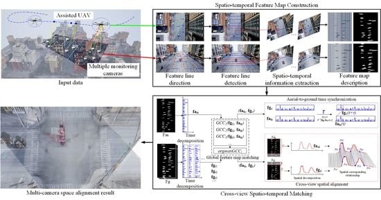
2. UAV-Assisted Wide Area Multi-Camera Space Alignment Based on Spatiotemporal Feature Map

Figure 2 provides an overview of the proposed UAV-assisted wide area multi-camera space alignment approach intuitively. With the videos from assisted-UAV and ground monitoring cameras as input, we first describe them by the spatiotemporal feature map, which lays a basis for multi-camera space alignment. Then, this paper puts froward a cross-view spatiotemporal matching strategy to mine the association relationship between these feature maps from multiple levels. The corresponding pixels between UAV-assisted videos and ground fixed videos can be obtained, and then multiple ground cameras are aligned into one surveillance space under UAV auxiliary data connection.
The following notations are used in this manuscript (Table 1).

2.1. Spatiotemporal Feature Map Construction

Before constructing spatiotemporal feature map, we firstly introduce the input data. As shown in Figure 2, the input data contains two parts: ground monitoring videos from ground deployed cameras and aerial videos from the UAV. Among them, each ground monitoring video corresponds to a deployed camera to be aligned. The aerial videos are collected by assisted UAV at different hover positions. The motion information in observation scene is contained in both UAV aided data and ground surveillance data, which is the key to motion consistency for subsequent cross-view matching.
Let N ground monitoring videos V C 1 , V C 2 , V C N denote the monitoring data from N deployed cameras, respectively, and V A 1 , V A 2 , V A M are the UAV-assisted data which are obtained by UAV hovering at M positions. How can these data be described by the spatiotemporal feature map? Similar to the general pipeline of visual feature construction (key point detection, feature extraction and description), our approach consists of three modules: feature line detection, spatiotemporal information extraction and feature map description.

2.1.1. Feature Line Detection

To find spatial correspondences between the UAV data and ground monitoring data, we expect to get the pixel relationship between them for camera space alignment. Therefore, local feature representation method is required for such local information matching. Similar to key point detection in widely-used SIFT algorithm, feature line detection is the beginning step in our proposed spatiotemporal feature map construction method.
What kind of line should we choose as feature line? As is known, there exists a great gap in perspectives between aerial UAV data and ground monitoring data. Perspective projection transformation causes deformation in length, relative proportion and intersection angle. That is why direct scene lines extracted by traditional hand-craft method or deep-learning network are not suitable for air-to-ground matching. However, fortunately, the intersection points of lines are precisely invariant under perspective projection transformation. According to this, we start with the establishment of feature lines. As shown in Figure 2, we draw several lines perpendicular to the direction of vehicle moving as feature lines. This is because such feature lines can capture rich visual intersection information of the moving target passing through them. Thsi intersection information remains unchanged between the air and the ground.
Considering the uncertainty of camera position and orientation, our approach adopts the combination of traffic flow direction and vanish point in [29] to determine feature line. Next, we introduce the proposed feature lines detection method of ground monitoring data and UAV-assisted data, respectively.
For ground monitoring data, feature line directions vary greatly in different camera orientations (Figure 3). When the camera faces the road center (Figure 3a), its feature line directions are quite similar. While for roadside camera, Figure 3b shows an instance of its collected data. The feature line directions are different in different positions. Their included angles are also different in two-dimensional image. Therefore, we need to determine the direction of feature line adaptively according to specific condition. By thoroughly analyzing scene visual information, feature line direction relates to the short edges of foreground moving vehicles. Their slope in different positions is the feature line direction. We adopt vanish point to help extract the feature line direction. This specific method was proposed by Dubská et al. [29], who first obtained the direction of traffic flows by optical flow and calculated the first vanish point by diamond space voting. The feature line corresponds to the direction parallel to the ground and perpendicular to the first direction. Thus, we model background edge to get the edge of foreground moving vehicle. Then, we filter out the edge which belongs to the first vanishing point or perpendicular to the ground. Feature lines are the extensions of these retained foreground edges.
As for aerial data from the UAV, its top view makes two-dimensional image without geometric perspective. That is different from ground monitoring data above. Therefore, the feature line direction is just the line perpendicular to the direction of traffic flow in two-dimensional image. Thus, in this part, we only utilize traffic flow detection to obtain feature line. To be specific, the procedure has two steps: traffic flow detection by optical flow approach and feature line drawing with vertical direction of optical flow. It is worth noting that aerial video usually has a wider observation range, which may involve traffic flow in multiple directions. For example, a turning road contains traffic in two directions. Multiple traffic directions correspond to multiple feature line sets. Feature lines in the same direction are grouped into one set.
Based on the methods stated above, we detect and draw feature line in N ground monitoring videos and M UAV-assisted videos. Each video has several feature lines. Taking V as a monitoring video example, it can come from ground cameras or aerial UAV. There are N L i feature lines detected from V. We finally obtain numerous ground feature lines and aerial feature lines after a series of the above-mentioned processing.

2.1.2. Spatiotemporal Information Extraction

This section aims to extract visual information from input ground monitoring data and aerial assisted data with the help of feature lines. According to motion consistency in cross-view data, we extract the visual information in two dimensions (temporal order and spatial structure). For temporal order extraction, the monitoring video is unframed in order. We record their spatial features from the feature line in turn. Thus, temporal visual feature shown over time can be extracted. Meanwhile, the visual changes in space are the spatial visual feature.
Figure 4 provides the detailed spatiotemporal information extraction method intuitively. Suppose f l i is one of the feature lines in monitoring video V; it is circled in this figure. V can be ground monitoring camera or aerial camera. The video is decoded into N i frames at the beginning. The visual data at the position and direction of this feature line can be found at corresponding locations in each frame. Next, the related data are extracted and integrated into one row in order. The number of rows is equal to the number of video frames, which is N i for f l i . Figure 4 (right) shows the rows from top to bottom corresponding to the video frames from front to back. The visual data of all rows are the spatiotemporal information extracted from feature line f l i .
The above visual information extraction approach not only extracts time series information at feature line location but also extracts spatial visual information on the different pixels of feature line. For better understanding, feature lines are similar to a door: the door can obtain what passed by recording what happened in every moment. Similarly, we can get what information go through the feature line by recording visual data in every frame. Thus, the motion time occurred as well as its space position are extracted.

2.1.3. Feature Map Description

Next, how to describe the above spatiotemporal information is also an important problem. To address this, we construct two dimensional feature map whose coordinate axes are the set of space and time information, respectively.
The spatiotemporal information extracted from the above section is represented by several visual data rows. Based on this, we then connect them in chronological order to form a two-dimensional feature map. The row of visual data calculated in the last section composes one row in the feature map, and the visual data at different time from one feature line position compose one column in the feature map. From the middle module of Figure 2, we can see that the time and position of every passed moving object are recorded in this feature map. The height of each moving object’s Y axis in feature map is their passage time through feature line, and the span of each moving object’s X axis is object width.
Then, we transform feature map into binary image with small data quantities by foreground object segmentation method. The benefits of this are the following. It can further highlight the motion information which is consistent in different cameras. At the same time, it can also filter out the other visual features that we do not care about (such as color and gradient). The feature map shows that most of the visual data in it are background road. Based on this, we start with the hypothesis that background occupies the majority relative to foreground motion. Then, each column in the feature map is processed as an independent unit to find the background of feature line. According to the statistical distribution of gray value in each column, the gray with maximum value comes from background. Thus, the pixel whose gray value is close to the maximum is set to 255 to indicate background, and vice versa. The binary processed feature map displays obvious black–white effect.
Thus far, the spatiotemporal feature map construction is finished. N ground monitoring videos V C 1 , V C 2 , V C N and M aerial assisted videos V A 1 , V A 2 , V A M are represented by spatiotemporal feature maps. The relationship of videos and their feature maps is one-to-many.

2.2. Cross-View Spatiotemporal Matching

To describe the proposed method clearly, we assume that the aerial spatiotemporal feature map from the UAV is query. To search for its matched database feature map from ground monitoring videos, we propose a cross-view spatiotemporal matching approach which can also determine the best space responding pixel between matched feature map pairs for camera space alignment. The proposed method includes three key steps: (1) global feature map matching; (2) aerial-to-ground time synchronization; and (3) cross-view spatial alignment. The first one measures the similarity of feature maps from the global and the latter two are used to find the corresponding relationship between local pixels.

2.2.1. Global Feature Map Matching

Let F a k be the kth query feature map from aerial assist UAV and F g the database which contains N g ground spatiotemporal feature maps. It is the collection of ground feature maps calculated from N ground monitoring videos V C 1 , V C 2 , V C N , as expressed in Equation (1). Figure 5 gives the whole global feature map matching method.
F g = { F g 1 , F g 2 , , F g N c 1 V C 1 , F g N c 1 + 1 , F g N c 1 + 2 , , F g N c 1 + N c 2 V C 2 , , F g N g }
First, the input feature maps F a k and F g are mapped into one-dimensional space before matching. The two-dimensional feature map matching problem is transformed into a one-dimensional feature vector similarity measurement problem. In doing so, it avoids complicated computing accompanied by high-dimensional feature maps while attempts to narrow the gap of 2D feature map caused by air-ground asynchronous. Our method projects 2D feature map to 1D feature vector in time (see Figure 2). To better describe this process, we take feature map F R m × n as an example. F is m rows and n columns. F can be regarded as several row vectors, as F = { r 1 , r 2 , , r m } . The number of row vectors is m and the dimension of each row vector is n. Each row vector comes from a sampling time. Then, as for each row vector, we count the number of foreground pixels as its feature number. Thus, a n-dimensional row vector is converted to a feature number. m row vectors are converted into m feature numbers. By arranging the m feature numbers in order, we can establish the time feature vector of feature map F. Thus, the two-dimensional feature map F, which is m rows and n columns, can be mapped to one-dimensional feature vector f t , which is an m-dimensional feature vector. The calculation process is shown as follows:
f t = { f t 1 , f t 2 , , f t m } , w h e r e f t j = c a r d ( r p ( q ) = 0 ) ; q = 1 , 2 , n ; p = 1 , 2 , m
In this way, query F a k is represented by fa t k , and all database feature maps in F g are also represented by time feature vectors. Our next step is to measure the similarity between them. The time non-synchronization problem among air and ground cameras makes the traditional Euclidean distance incapable of quantifying their similarity. This paper analyzes the generalized cross-correlation value between them as the similarity measurement. We adopt the evaluation index of generalized cross-correlation. It was defined by Cobos [30] in 2020, who improved the general generalized cross-correlation based on the sub-band analysis of cross-power spectrum phase, named FS-GCC (Frequency-sliding Generalized Cross Correlation). This method shows robust performance under noise and reverberation. Concretely, according to their denoised FS-GCC values based on weighted SVD, the similarity between query feature vector fa t k and every database feature vector in fg can be obtained. In the following calculation, the highest scoring database feature vector is the ground feature vector matched with fa t k . We denote it as fg t i . Meanwhile, their corresponding feature maps F a k and F g i are a matched pair.
i = a r g m a x p ( FS GCC ( fa t k , fg t p ) ) w h e r e fg t p fg
When all aerial feature maps retrieve their matched ground feature maps in database, we can obtain several feature map pairs, which are the results of global feature map matching. Furthermore, the feature lines corresponding to the same feature map pair are considered as a matched feature line pairs.
After finding the matching relationship between feature maps globally, we next try to find the correspondence between local pixels. The calculation procedure includes two key modules: aerial-ground time synchronization and cross-view spatial alignment.

2.2.2. Aerial-to-Ground Time Synchronization

To find the corresponding pixels between matched feature line pairs, we need to realize time synchronization between them at first. The visual feature is described by spatiotemporal feature maps in this paper, time synchronization and space alignment are closely related. Time synchronization affects the accuracy of finding corresponding points, and then influences the performance of camera spatial alignment. In other words, considering a single variable principle, accurate spatial correspondence is obtained under the prior time unification of spatiotemporal feature maps.
Mathematically, feature vectors fa t k and fg t i are one-dimensional time features enriched from the two-dimensional feature maps F a k and F g i . They are also the time series. The problem of feature maps’ time synchronization is also the issue of one-dimensional series’ time delay estimation. Generalized cross correlation is one of the most commonly used method. It estimates time delay by analyzing the correlation between two signals. Therefore, our approach employs an improved generalized cross correlation algorithm [30] to synchronize fa t k and fg t i . This method is used for similarity measurement and global match feature map matching in the previous section. In terms of time delay estimation of fa t k and fg t i , their concrete time delay τ is the corresponding value when the maximum cross-correlation value obtains. Let G be the calculation function ( G named W S V D F C G C C in [30], and we do not bore you with its details), the time delay can be calculated as below:
τ ^ = a r g m a x τ G ( fa t k ( t ) , fg t i ( t + τ ) )
τ ^ is the time delay of aerial feature vector fa t k and ground feature vector fg t i . fa t k is the reference. The first component of fa t k and the τ ^ th component of fg t i are synchronized. We reverse τ ^ into the row of feature maps F a k and F g i , and the collection time of these rows is the same. We than cut the same length T from the synchronization row and get new spatiotemporal feature maps F a k R T × n a and F g i R T × n g . The parameter T needs to meet the following two requirements: T < m a and T + τ ^ < m g . The specific calculation method is expressed as:
F a k = F a k A w h e r e F a k R m a × n a ; F a k R T × n a ; A R ( m a T ) × n a
F g i = B F g i C w h e r e F g i R m g × n g ; F g k R T × n g ; B R τ ^ × n a R ( m g T τ ^ ) × n a

2.2.3. Cross-View Spatial Alignment

With F a k and F g i , we next solve the problem of finding corresponding pixels for cross-view spatial alignment. Our proposed method includes three steps: (1) feature map dimension reduction; (2) one-dimensional space feature vector alignment; and (3) cross-view air-to-ground spatial alignment.
Similar to Section 2.2.1 that maps feature map to time dimension, we map F a k = { ca 1 T , ca 2 T , , ca n a T } and F g i = { cg 1 T , cg 2 T , , cg n g T } to space dimension at first. Figure 6 displays the proposed feature dimension reduction and alignment process vividly. As we can see, F a k and F g i are reduced to one dimension as space feature vectors fa s k and fg s i . The length of space feature vector is equal to the number of columns in feature map and each component is the number of foreground pixels in the corresponding column. The calculation formula is as follows.
fa s k = { f a s k 1 , f a s k 2 , , f a s k n a } w h e r e f a s k p = c a r d ( ca p ( q ) = 0 ) ; q = 1 , 2 , T ; p = 1 , 2 , n a
fg s i = { f g s i 1 , f g s i 2 , , f g s i n g } w h e r e f g s i p = c a r d ( cg p ( q ) = 0 ) ; q = 1 , 2 , T ; q = 1 , 2 , n g
Note that the length of space feature vectors are different because the different sizes of feature maps.
We leverage Dynamic Time Warping ( D T W ) [31] as the matching method to align a pair of space feature vector fa s k and fg s i . It is a simple but effective template matching algorithm which is also universality for different sequence lengths. Our first stage is to construct a distance matrix D R n a × n g . D ( x , y ) is the Euclidean distance between the xth element of fa s k and the yth element of fg s i . After that, we start to align the two sequences. The matching path is set as W = w 1 , w 2 , , w j , , w l ( m a x ( | n a | , | n g | ) l | n a | + | n g | ) . Each element w j = ( x , y ) represents the aligned coordinate pair (xth coordinate of fa s k aligns with the yth coordinate of f g s i ). To ensure each element in the sequence can find its corresponding alignment position without intersection, W needs to satisfy:
w 1 = 1 , 1
w l = n a , n g
w j + 1 = ( x , y ) x x x + 1 y y y + 1
where x and y are the next matched coordinates of fa s k and fg s i . It only has three possible results: ( x + 1 , y ) , ( x , y + 1 ) , ( x + 1 , y + 1 ) . We choose the one with the minimum cumulative distance from ( x , y ) according to distance measurement D. After that, we can obtain the matching relationship between vector elements which is stored in W . However, there are diversified corresponding relation types which include one-to-many relationship, many-to-one relationship and one-to-one relationship. The first two are ambiguous in spatial alignment, so we only retain the one-to-one matching pixel pairs. At the same time, we further sample these one-to-one pixel pairs at equal space intervals to get sparse space correspondences. After such screening, W is the corresponding coordinate set between fa s k and fg s i .
Feature maps F a k and F g i constructed by fa s k and fg s i are just an example of matched feature map pairs. All feature map pairs calculated after Section 2.2.1 can obtain their corresponding relationship between local pixel by the methods in Section 2.2.2 and Section 2.2.3. Thus, several corresponding coordinate sets are returned. Moreover, we can track back to the feature line and camera corresponding to each set. This means that we obtain several cross-view corresponding points between aerial 2D images captured by assisted UAV and ground 2D visual data collected by deployed monitoring cameras.
Once air-to-ground corresponding pixels are matched, we calculate the homography matrix between cameras by more than four non-collinear corresponding coordinate pairs. The relative projection relationship between them can be estimated. In this way, the proposed method gets the relationship between each ground monitoring camera and the assisted UAV. The M locations of assisted UAV can be united into one coordinate system with current visual positioning and navigation methods (e.g., SLAM), so ground deployed cameras are aligned to this coordinate system naturally. Our system realizes multi-camera space alignment in large scale environment under UAV assistance.

3. Experiments

We conducted extensive experiments to evaluate the performance of our proposed multi-camera space alignment approach based on spatiotemporal feature map. To maintain the objectivity and comprehensiveness, we constructed an evaluation database by ourselves, which is described in Section 3.1. On this basis, we then explored the robustness and accuracy of our proposed method from both qualitative and quantitative aspects in simulation environment and real scene. The extended applications of our approach are provided in Section 3.4.

3.1. Database

  • Database in simulation environment
This paper utilizes AirSim [32] as the simulation platform to construct a suitable virtual scene for our system’s performance verification. AirSim is an open source simulator based on Unreal Engine. It supports cross-platform operation, multiple programming languages and various sensors (camera, UAV, Lidar, GPS, etc.). Some major parameter settings in Airsim are summarized in Table 2, including environmental parameters and sensor parameters. Figure 7 presents the simulation scene model and some simulation monitoring data.
To be specific, we chose a model of urban street block as our simulation environment, as shown in Figure 7a. It includes abundant and complex city elements: buildings, landscape plants, traffic signs, junctions, etc. Based on this model, we firstly load multiple car models and set various running routes to restore the real traffic flow as much as possible. Then, the camera model and UAV at different positions are added to imitate ground monitoring cameras and aerial auxiliary camera. Thereafter, we collect simulation monitoring data with these cameras and establish a test simulation dataset called C a m D a t a S i m . This database consists of two parts: (1) 24 videos from 11 ground cameras at fixed locations; and (2) 5 aerial videos from the UAV at 5 hover positions. Their frame resolution and rate are set to 1920 × 1080 and 25 fps, respectively. The self-built simulation database C a m D a t a S i m is provided in Figure 7 (right). Several vehicles shuttle through these streets and their moving information is collected into ground monitoring videos and the UAV videos independently. Moreover, to better evaluate the effectiveness of the proposed method, these videos are captured by ground cameras and UAV at different heights with different pitch angles.
  • Database in real scene
Taking into account that current public multi-camera databases cannot provide both ground monitoring data and auxiliary UAV data, we constructed a new multi-camera monitoring database. Figure 8 provides the collection environment and data of our self-built database. Table 2 provides its related parameter settings, in which some cannot be obtained in real scenes and only roughly estimated parameters are given. (1) Acquisition environment: This database is collected from a mixed traffic system with bidirectional six-lane main road and bidirectional four-lane side road. The width of its middle green belt is about 25 m and the total transverse length of this road is more than 60 m. (2) Camera configuration: There are four ground monitoring cameras and each camera monitors traffic in one traffic area, including northbound main road, northbound side road, southbound main road and southbound side road. Since the accurate parameters of a deployed multi-camera system are unknown, we make a rough estimation of its main parameters. The deployment heights of ground cameras are about 7 m and their pitch angle is about 60°. As shown in Figure 8, there is little overlap between their field of view. The auxiliary UAV data which overlook the observation scenario are captured at about 80 m. It contains common motion information with the ground monitoring data. (3) Data information: The frame resolution and rate of all data in this database are 1920 × 1080 and 25 fps, respectively. The total frame number of each ground video is 5493. The time delay and space relationship between these data is unknown. This paper applies the proposed approach to estimate the space alignment relationship between the ground cameras with UAV assistance.

3.2. System Performance Evaluation on Simulation Environment

In this section, we explore the performance of our proposed approach on three typical traffic scenarios: crossroad, T-junction and straight road. In addition to qualitative analysis, we also conduct quantified analysis on simulation environment in which the ground truth is manually labeled. Figure 9 displays some space alignment results and Table 3 the pixel error statistics.
Figure 9 shows the space alignment results of crossroad, T-junction and straight road, from top to bottom, respectively. The fist column is the monitoring data of ground deployed cameras. They are transformed into the united coordinate system with the alignment parameter. The following error analysis roughly evaluates algorithm performance by the coincidence degree between ground truth (marked in green) and our results (marked in red). Multi-camera space alignment results are shown in the end. It can be seen in this figure that our approach performs well in different situations. The first simulation scene is a crossroad. Four overlapping monitoring cameras monitor traffic from four directions. To better see the space alignment performance of overlapping region, the space alignment results of crossroad are set to translucent. Compared with ground truth, we can find that zebra crossings are mapped together successfully. That means the same visual information is aligned to the same coordinates, which indicates the effectiveness of our approach. The second simulation scene is a T-junction and the ground monitoring cameras in it have limited overlapping area between them. Under UAV assistance, these three cameras are calibrated into one space. This illustrates that our system can maintain stable performance with partial-overlapping cameras. The bottom test situation is a straight road with three cameras of sequential distribution. Their overlapping region is not only limited but has fewer visual features. As the right column shows, we can return good space alignment results, further verifying the robustness of our proposed method.
The quantitative experimental study was conducted by analyzing the pixel error between our space alignment results and ground truth. Table 3 shows that the pixel error varies from 5.78 to 23.76 pixels. The average errors on above three scenarios are 20.02, 20.32 and 10.01 pixels, respectively. Thus, if we want to relate the visual data of different cameras, the space alignment error is within 25 pixels. This set of evaluations on different monitoring scenes further demonstrates that the proposed approach satisfies the need in the practice interconnection application. Meanwhile, these quantitative results are also in good agreement with the previous qualitative results. In addition, we can see in this table that there are some differences of space alignment error between different scenarios. The performance of straight road is better than that of crossroad and T-junction. The reason for this phenomenon is as follows. Crossroad and T-junction have both turning and straight traffic. They include more complex motion compared with straight road. This leads to more disturbances of feature line detection and spatiotemporal feature map construction, which directly influences space alignment performance.
Overall, the evaluation in a simulation environment shows that our proposed multi-camera space alignment approach obtains satisfactory performance not only in quality but also in quantity.

3.3. System Performance Evaluation on Real Environment

Besides evaluation on simulation environment, we also evaluated the performance of our system in a real environment. The test scene and monitoring data constructed by ourselves is introduced in detail in Section 3.1. We applied the proposed method to align the four ground monitoring cameras into one united coordinate system.
Figure 10 shows our space alignment result in real traffic scene. The monitoring data from four ground cameras are mapped into a united coordinate system, as shown in the second column. We then compare our result (labeled in red) with ground truth (labeled in green by manual calibration) qualitatively. The comparison results of the individual camera and the whole system are both provided. Viewing the result as a whole, we can see that these ground cameras are well aligned. Their space alignment results replay the whole monitoring scene, which is a bidirectional traffic system with greenbelt. The imaging relationship between these limited overlapping ground cameras can be obtained with UAV connection. This means that cameras can cooperate for overall surveillance. By comparing with the ground truth, the pixel error of our approach is about 20, which demonstrates the feasibility and effectiveness in real environment. From a local point, lane direction after each camera mapping is basically parallel. That conforms to the actual situation, which also confirms algorithm performance. However, as we can see, our approach performs poorly on the distant targets which are warped incorrectly with too large longitudinal extension. This happens because our method cannot get enough feature lines when the object is too small in the far region.
The above experiments were conducted on a computer with an Interl(R) Core(TM) i9-9900X (3.50 Hz GPU, NVIDIA GeForce GTX 1080Ti GPU, 64 GB RAM) using C++. The computational complexity of the proposed method is analyzed below. As described, the proposed method contains two main modules: spatiotemporal feature map construction and cross-view spatiotemporal matching. For the real scene above, the running time of the first module is about 123.9 s. In the second module, the feature map dimensional reduction in time and space costs 38.2 s on average. The time of air-to-ground time synchronization and cross-view spatial matching is 136.0 s. To sum up, the time cost to align the ground monitoring cameras in the above real scene is within 5 min. That also verifies the fast spatial alignment ability of our system in large scenes. In addition, the proposed method is easier to operate in real environment. The operation complexity mainly comes from input data preparation. The input ground monitoring videos can be obtained from database or real-time monitoring data. The UAV needs to capture the monitoring space from top view under stable flight condition. We only need a part of the common motion information between ground and aerial data and do not require data synchronization.

3.4. Extended Applications

Due to its multi-camera space alignment ability, the proposed method has great value in many real-world scenarios. For example, vehicle road hybrid system is a common traffic scene. Multiple cameras are used in it to monitor traffic operation status. The proposed method can be applied to estimate the space relationship between cameras and converts independent monitoring to integrated monitoring. The efficiency of traffic monitoring can be improved. A campus is a typical example of our approach’s application scenario. To insure teachers and students work or study on a harmonious campus, many cameras are deployed in every corner of the campus. The proposed method can be used to obtain the spatial position of each camera in a campus and unify them into a coordinate system. Thus, all monitoring data will be aligned as a whole. We can see what is happening on campus from the whole multi-camera video rather than multiple separate single camera videos. Besides the above two examples, our approach also can be applied to key industrial factories, large-scale activity square, etc.
In addition, the proposed method, which lays the foundation of multi-camera system, has the potential application value in many multi-camera cooperation fields, including object re-identification, multi-object detection, multi-camera cooperative locating, and so on. To be specific, on the basis of our multi-camera space alignment results, cross-camera object re-identification can be solved from a new perspective. Other object re-identification methods identify the same target by their feature similarity. Unlike other methods that mine their similarity, we can relate the same object across different cameras by the estimated spatial corresponding relationship. Furthermore, the initial object detection result can be verified by multiple cameras with their space alignment result. Through the spatial correspondence between target boxes, false alarm rate and missed rate can also be reduced. For multi-camera cooperative locating, their space alignment result can provide a references location of the interested target. Especially, when the target is occluded, the result obtained by our approach can ensure stable positioning accuracy.
To show the utility of our proposed approach in real-world intuitively, we apply it in a typical vehicle road hybrid system. Figure 11 shows a crossroad with four ground monitoring cameras. They observe the traffic intersection from four directions. The proposed method has application value in imaging display and intelligent analysis. Concretely, on the one hand, the proposed method aligns the four cameras into one coordinate system. Four independent monitoring videos are unified into a more comprehensive monitoring video, as shown on the right. That allows users to timely obtain the whole intersection running state, which improves the efficiency of current video surveillance. On the other hand, the spatial correspondence between different cameras obtained by our approach also contributes to cross-camera intelligent analysis. If we employ single camera object detection algorithm on one of these cameras, the objects can be detected out. As shown in the upper left corner, a white car marked with red box is detected out. On the basis of our result, the data of this target in other cameras can be directly associated. In other words, such ability to relate targets across cameras is capable of cross-camera re-identification and tracking. Compared with other methods which detect objects in different cameras separately first and then re-identify them, our approach only detects objects of one camera and relate them by coordinate correspondence. The efficiency and robustness of cross-camera intelligent analysis are naturally improved.

4. Discussion

4.1. Performance Comparison

In this section, we compare our performance with other works from two levels. First, from the partial important sub-process, we conducted contrast experiments on cross-view matching performance, which is one of the key technologies in our system. Then, from the overall performance, we compared our approach with other methods on multi-camera space alignment.

4.1.1. Comparison of Cross-View Matching

Cross-view matching, which mines the relationship between ground monitoring camera and auxiliary UAV, is one of the key technologies involved in this paper. Its accuracy has a direct impact on air-to-ground coordinate system unification, and thus plays a negative role in multi-camera space alignment. Therefore, first, the performance our proposed cross-view matching algorithm is compared with other matching methods in both simulation and real environments.
SIFT (Scale-Invariant Feature Transform) [33] proposed by Lowe and SuperGlue [34] proposed by Sarlin are chosen as the contrast methods. SIFT as a traditional hand-crafted matching approach that is widely used in practical application. It extracts local feature from input image and measures them similarity by Euclidean distance. The highest scoring feature and query feature are the matching pair. SIFT is robust to rotation, zoom scale and brightness changes. SuperGlue [34], as a deep neural matching network, was recently proposed. It is based on graph neural network and attention mechanism. They regard matching as the optimal transport problem in which the loss function is constructed by deep network. In the specific implementation, two images and their visual features described by SuperPoint [35] are the input. They are then sent to the matching network established by SuperGlue and the matching relationship between them is returned as output.
Figure 12 shows the qualitative performance comparison of SIFT, SuperGlue and our approach on cross-view matching. The test image on the left is a UAV aerial image, and its related ground monitoring image is provided on the right. They observe the monitoring scene from the top view and street view, respectively. Obviously, there exists great perspective gap between them. The evaluation results on simulation environment and real traffic scene are provided from top to bottom.The above three methods are applied on the two scenes for cross-view matching. For visualization, the matching pairs found by each method are connected with straight lines. We can see that our proposed method outperforms the other methods in both quantity and accuracy. (1) For quantity, our approach returns more than 60 matching pixel pairs. SIFT only obtains a few matching pairs. SuperGlue finds plenty of matching pairs in the simulation environment, but it finds very few pairs in real scene. (2) For accuracy, most of the matching pairs calculated by SIFT are not correct. Similarly, SuperGlue can also hardly find the accurate cross-view corresponding point. However, in the matching results of our system in the simulation and real environments, the overwhelming majority of pairs are accurate. According to the above analysis, SIFT gets too few and incorrect matching pairs. The accuracy of SuperGlue is also poor on air-to-ground matching. In other words, the two approaches fail on cross-view matching. However, our proposed method can obtain sufficient and correct matching pairs. It shows satisfying performance across different perspective views.
The high performance of our approach is due to the proposed spatiotemporal feature map and cross-view matching method, which links up different views according to intersection invariance of projection transformation. Thus, it is naturally robust to view change. However, SIFT matches images by their local feature similarity. That makes it difficult to cover such huge view gap. Meanwhile, there are many similar elements in the observation scene, e.g., the pedestrian crossings in four directions. That is also a key reason for the poor performance of SIFT. SuperGlue is based on a pre-trained matching network. Its performance depends on the scale and quality of the training database. The disadvantage of matching neural network on generalization capability causes its failure of cross-view matching. To sum up, experimental evaluation and result analysis prove that our approach has better performance than the comparison methods in cross-view matching.

4.1.2. Comparison of Multi-Camera Space Alignment

For the overall multi-camera space alignment performance, we compare the proposed method with other two methods: COLMAP and MapNet.
COLMAP is a widely used 3D reconstruction approach based on structure-from-motion [36] and multi-view stereo [37]. Without camera calibration in advance, COLMAP can reconstruct the whole scene with a set of ordered or unordered two-dimensional images. For multi-camera space alignment, we use COLMAP to reconstruct the whole monitoring scene by inputting a series of scene images obtained from different angles. Then, the monitoring data from multiple ground camera as the new registered images can be re-localized into scene reconstructed model. Thus, multiple cameras are united into the coordinate system established by scene reconstructed model. Thus, COLMAP can also achieve multi-camera space alignment based on three-dimensional reconstruction.
MapNet [38] is a camera localization approach with geometry-aware learning of maps. It was proposed by Brahmbhatt in 2018. In this work, they proposed a novel parameterization method for camera rotation to better estimate camera pose with deep learning network. In other words, MapNet can be regarded as an end-to-end multi-camera method. The ground monitoring data can be sent to this network and the output is each camera’s pose in the whole scene map. The relative space relationship is also contained in their poses. On the basis of multiple camera localization, we can align them. Therefore, MapNet can realize multi-camera space alignment by camera localization.
As described above, COLMAP and MapNet are not proposed for multi-camera space alignment. The reason that we choose them as the comparison methods are as follows. First, the related works for overlapping cameras and non-overlapping cameras are not suitable for comparison. The overlapping relationship between cameras in wide area multi-camera system is usually chaotic and unknown. Marker- or motion-based methods can estimate camera spatial topological relations and not the pixel level correspondence. Second, COLMAP as a representative algorithm of 3D reconstruction and MapNet as a deep learning method can obtain camera space relationship in some ways. They can implement multi-camera space alignment with data post processing. The comparison with them can reflect the performance of our method on space alignment.
The multi-camera space alignment results of the above three methods are displayed in Figure 13. As we can see, the test scene is a crossroad with four ground monitoring cameras. From left to right, the results of COLMAP, MapNet and ours are provided. COLMAP successfully aligns the monitoring data captured from four cameras into one coordinate. The same visual information (e.g., the zebra crossings) is mapped with the same two-dimensional coordinate. As for MapNet, it fails to align all monitoring data into one united coordinate system. Especially, the result of Camera 2 maps the data into the wrong coordinates. That leads to a large pixel error with manually labeled ground truth. Meanwhile, the final alignment result is also formless, which makes it hard to monitor the scene in all directions. The alignment result obtained by our proposed method shows comparable qualitative performance with COLMAP. The four monitoring cameras are also well aligned into one united coordinate system. We can see that the error between ground truth and our result is very small. To quantitative compare the pixel error, we statistically analyze the error of each method, as shown in Table 4. It is the qualitative experiment results. COLMAP obtains the minimum pixel error on each camera space alignment, while MapNet has quite large pixel error. The pixel error of our approach is about 20 pixels, which can meet the demand in real-world.
The factors causing the above results are analyzed below. The high performance of COLMAP is due to the space relationship provided by its pre-built scene 3D model. A better scene model guarantees accurate space alignment. However, such scene model is usually obtained by a variety of scene images, requiring 10 h for three-dimensional reconstruction. With the increase of the number of cameras and monitoring area, it will take more time. It cannot meet the needs of fast spatial alignment in large scenes. The performance of MapNet is limited by the deep neural network. It can regress camera pose by multi-layer network computing and pre-data training. However, such pose regression method still has accuracy disparity with the method based on geometry structure and image retrieval. For the proposed method, it ensures space alignment efficiency with the help of UAV, which has excellent flexibility and global awareness that can adapt to the needs of fast spatial alignment in large scenes. Meanwhile, we mine the motion consistency between UAV and ground monitoring cameras. Thus, we can align them into one united coordinate system by air-to-ground pixel correspondence. That ensures the space alignment accuracy. To balance the efficiency and accuracy, our approach returns better performance than the other contrast methods.

4.2. Parameter Discussion

This section discusses the effect of three parameters on our system’s performance: the number of feature lines, camera pitch angle and deployment height. The number of feature lines relates to cross-view visual feature extraction and description. Different camera pitch angles and deployment heights are also two main factors influencing our performance.
The evaluation data are captured from a typical crossroad on simulation environment, as presented in the top of Figure 9. To simulate different situations, we vary the view angle and deployment height of ground cameras. Meanwhile, the number of feature lines is also changed to analyze algorithm performance. Using variable-controlling principle, the pixel errors by varying these parameters are studied. The experimental results are given in Figure 14. It provides the proposed method’s pixel error under different camera pitch angles (20°, 30° and 40°) and different camera deployment heights (5 and 9 m) with different number of feature lines (the range interval is [ 50 , 600 ] ).
First, the error decreases with increasing the parameter of number of feature lines, as shown by the three curves. When this number is large enough, the algorithm error keeps at a low level. That is because more feature lines mean more spatiotemporal feature maps. The input data can be described more comprehensively, and then rich cross-camera corresponding points can be obtained. Thus, the accuracy is greatly improved at the beginning. However, when we have enough features and corresponding points, the error will not be greatly reduced. An appropriate number of feature lines for the proposed method is about 200–300. At the same time, it can be seen that the greater is the camera pitch angle, the better is the performance. Overall, 40° obtains the minimum alignment error. Large pitch angles of the ground monitoring camera have a small perspective gap between it and the aerial UAV. That makes air-to-ground matching more accurate and further improves multi-camera space alignment performance. In addition, we also found that the situation with 40° pitch angle converges to the minimum error more slowly than others. Under the same deployment height, the more the camera looks down, the smaller its observation range is. Therefore, it requires more feature lines for accurate space alignment.
The blue and green curves show the impact of different deployment heights on alignment error. We enlarge the error results after convergence in the upper right corner. It is noticeable that the space alignment error of cameras deployed at 9 m is lower than those at 5 m. It is for the same reason that a large pitch angle has a smaller error. High deployed cameras have more similar perspective views with auxiliary UAV. They can be aligned into the united coordinate system established by UAV more accurately. The change regularity of feature line number also verifies the discussion in the previous paragraph.
However, there are two major limitations to this study that will be addressed in the future. First, the proposed multi-camera space alignment approach is based on UAV-assisted aerial data, which unifies ground monitoring cameras. Thus, it is not applicable to these monitoring situations where stable UAV video cannot be obtained, e.g., no fly zone for UAV, bad weather so the UAV is unable to hover stably or areas that are covered by trees or other things. Secondly, the performance of our proposed method depends on the spatiotemporal feature map which describes input data with abundant traffic flow. However, it is affected by random traffic flow. When the passing vehicles are too sparse or their moving direction is complex, our system performs poorly. To overcome this problem, lane detection and segmentation can be used to reduce dependence on traffic flow during future work.

5. Conclusions

This paper introduces a novel UAV-assisted wide-area multi-camera space alignment approach based on a spatiotemporal feature map. The proposed methods contains two key parts: spatiotemporal feature map construction and cross-view space matching. The first is presented on the basis of motion consistency between UAV-assisted aerial data and ground monitoring data. Following the procedure of feature line detection, spatiotemporal information extraction and feature map description, all input monitoring videos are described by spatiotemporal feature maps. The second key module is the cross-view space matching strategy, which is proposed to find the corresponding relationships between aerial and ground data. Through three matching steps, which are global feature map matching, air-to-ground time synchronization and cross-view spatial alignment, we can obtain a set of air-to-ground corresponding pixel pairs. In this way, the spatial relationship between assisted UAV and ground deployed camera can be calculated. Due to the united coordinates between UAVs, multiple cameras are successfully aligned into one coordinated system with UAV assistance.
Experimental results on simulation environment and real scene demonstrate that our system achieves satisfactory performance and aligns multiple camera in one space coordinate system. From the quantitative analysis, its minimum pixel error is around 5 pixels and the maximum error is less than 25 pixels. Through parameter discussion, we find that high deployment height and large pitch angle of camera are beneficial to alignment accuracy. Meanwhile, the proposed method shows superior performance to other contrast methods. Furthermore, this study has great academic meaning for camera pose estimation, camera array imaging and cross-camera information fusion. It has significant application value in the field of traffic monitoring, public security and so on. However, there may be some possible limitations to this study. The proposed method cannot work in no UAV fly zones which cannot obtain UAV-assisted data. Because the proposed method relies on traffic flow, it not applicable to the area with not enough traffic. Our future work will consider these problems.

Author Contributions

Conceptualization, J.L., Y.X., C.L. and T.Y.; Data curation, J.M. and Z.D.; Formal analysis, C.L.; Funding acquisition, J.L.; Methodology, J.L., Y.X. and T.Y.; Resources, Y.X.; Validation, J.M. and Z.D.; Writing—original draft, C.L.; and Writing—review and editing, J.L., Y.D. and T.Y. All authors have read and agreed to the published version of the manuscript.

Funding

This research was funded by National Natural Science of China (Nos. 62073262 and 61672429), Key Research and Development Program of Shaanxi (No. S2021-YF-ZDCXL-ZDLGY-0127), the Fundamental Research Funds for the Central Universities and the Innovation Fund of Xidian University (No. 20109205456).

Institutional Review Board Statement

Not applicable.

Informed Consent Statement

Not applicable.

Data Availability Statement

The data and the details regarding where data supporting reported results in this paper are available from the corresponding author.

Conflicts of Interest

The authors declare no conflict of interest.

References

  1. Tang, Z.; Naphade, M.; Liu, M.; Yang, X.; Birchfield, S.; Wang, S.; Kumar, R.; Anastasiu, D.C.; Hwang, J. CityFlow: A City-Scale Benchmark for Multi-Target Multi-Camera Vehicle Tracking and Re-Identification. In Proceedings of the IEEE Conference on Computer Vision and Pattern Recognition, Long Beach, CA, USA, 15–20 June 2019; pp. 8797–8806. [Google Scholar]
  2. Yang, T.; Li, Z.; Zhang, F.; Xie, B.; Li, J.; Liu, L. Panoramic UAV Surveillance and Recycling System Based on Structure-Free Camera Array. IEEE Access 2019, 7, 25763–25778. [Google Scholar] [CrossRef]
  3. Deng, H.; Fu, Q.; Quan, Q.; Yang, K.; Cai, K. Indoor Multi-Camera-Based Testbed for 3-D Tracking and Control of UAVs. IEEE Trans. Instrum. Meas. 2020, 69, 3139–3156. [Google Scholar] [CrossRef]
  4. Yang, T.; Ren, Q.; Zhang, F.; Xie, B.; Ren, H.; Li, J.; Zhang, Y. Hybrid Camera Array-Based UAV Auto-Landing on Moving UGV in GPS-Denied Environment. Remote Sens. 2018, 10, 1829. [Google Scholar] [CrossRef] [Green Version]
  5. Hsu, H.; Wang, Y.; Hwang, J. Traffic-Aware Multi-Camera Tracking of Vehicles Based on ReID and Camera Link Model. In Proceedings of the 28th ACM International Conference on Multimedia, Seattle, WA, USA, 12–16 October 2020; pp. 964–972. [Google Scholar]
  6. Cai, W.; Yang, J.; Yu, Y.; Song, Y.; Zhou, T.; Qin, J. PSO-ELM: A Hybrid Learning Model for Short-Term Traffic Flow Forecasting. IEEE Access 2020, 8, 6505–6514. [Google Scholar] [CrossRef]
  7. Truong, A.M.; Philips, W.; Deligiannis, N.; Abrahamyan, L.; Guan, J. Automatic Multi-Camera Extrinsic Parameter Calibration Based on Pedestrian Torsors . Sensors 2019, 19, 4989. [Google Scholar] [CrossRef] [Green Version]
  8. Khoramshahi, E.; Campos, M.B.; Tommaselli, A.M.G.; Vilijanen, N.; Mielonen, T.; Kaartinen, H.; Kukko, A.; Honkavaara, E. Accurate Calibration Scheme for a Multi-Camera Mobile Mapping System. Remote Sens. 2019, 11, 2778. [Google Scholar] [CrossRef] [Green Version]
  9. Yin, L.; Luo, B.; Wang, W.; Yu, H.; Wang, C.; Li, C. CoMask: Corresponding Mask-Based End-to-End Extrinsic Calibration of the Camera and LiDAR. Remote Sens. 2020, 12, 1925. [Google Scholar] [CrossRef]
  10. Castanheira, D.; Silva, A.; Gameiro, A. Set Optimization for Efficient Interference Alignment in Heterogeneous Networks. IEEE Trans. Wirel. Commun. 2014, 13, 5648–5660. [Google Scholar] [CrossRef] [Green Version]
  11. Lv, F.; Zhao, T.; Nevatia, R. Camera Calibration from Video of a Walking Human. IEEE Trans. Pattern Anal. Mach. Intell. 2006, 28, 1513–1518. [Google Scholar] [PubMed]
  12. Liu, J.; Collins, R.; Liu, Y. Surveillance Camera Autocalibration based on Pedestrian Height Distributions. In Proceedings of the British Machine Vision Conference, Dundee, UK, 29 August–2 September 2011; pp. 1–11. [Google Scholar]
  13. Liu, J.; Collins, R.T.; Liu, Y. Robust Autocalibration for A Surveillance Camera Network. In Proceedings of the 2013 IEEE Workshop on Applications of Computer Vision, Clearwater Beach, FL, USA, 15–17 January 2013; pp. 433–440. [Google Scholar]
  14. Bhardwaj, R.; Tummala, G.K.; Ramalingam, G.; Ramjee, R.; Sinha, P. AutoCalib: Automatic Traffic Camera Calibration at Scale. ACM Trans. Sens. Netw. 2018, 14, 19:1–19:27. [Google Scholar] [CrossRef]
  15. Wu, F.; Hu, Z.; Zhu, H. Camera Calibration with Moving One-dimensional Objects. Pattern Recognit. 2005, 38, 755–765. [Google Scholar] [CrossRef]
  16. Zhang, Z. A Flexible New Technique for Camera Calibration. IEEE Trans. Pattern Anal. Mach. Intell. 2000, 22, 1330–1334. [Google Scholar] [CrossRef] [Green Version]
  17. Abdel-Aziz, Y.I.; Karara, H.M. Direct Linear Transformation from Comparator Coordinates into Object Space Coordinates in Close-Range Photogrammetry. Photogramm. Eng. Remote Sens. 2015, 81, 103–107. [Google Scholar] [CrossRef]
  18. Marcon, M.; Sarti, A.; Tubaro, S. Multi-camera Rig Calibration by Double-sided Thick Checkerboard. IET Comput. Vis. 2017, 11, 448–454. [Google Scholar] [CrossRef]
  19. Unterberger, A.; Menser, J.; Kempf, A.; Mohri, K. Evolutionary Camera Pose Estimation of a Multi-Camera Setup for Computed Tomography. In Proceedings of the IEEE International Conference on Image Processing, Taipei, Taiwan, 22–25 September 2019; pp. 464–468. [Google Scholar]
  20. Huang, L.; Da, F.; Gai, S. Research on Multi-camera Calibration and Point Cloud Correction Method based on Three-dimensional Calibration Object. Opt. Lasers Eng. 2019, 115, 32–41. [Google Scholar] [CrossRef]
  21. Yin, H.; Ma, Z.; Zhong, M.; Wu, K.; Wei, Y.; Guo, J.; Huang, B. SLAM-Based Self-Calibration of a Binocular Stereo Vision Rig in Real-Time. Sensors 2020, 20, 621. [Google Scholar] [CrossRef] [PubMed] [Green Version]
  22. Mingchi, F.; Panpan, J.; Yibo, L.; Jingshu, W. Research on Calibration Method of Multi-camera System without Overlapping Fields of View Based on SLAM. J. Phys. Conf. Ser. 2020, 1544, 012047. [Google Scholar]
  23. Xu, Y.; Gao, F.; Zhang, Z.; Jiang, X. A Calibration Method for Non-overlapping Cameras based on Mirrored Absolute Phase Target. Int. J. Adv. Manuf. Technol. 2019, 104, 9–15. [Google Scholar] [CrossRef] [Green Version]
  24. Mingchi, F.; Shuai, H.; Jingshu, W.; Bin, Y.; Taixiong, Z. Accurate Calibration of A Multi-camera System Based on Flat Refractive Geometry. Appl. Opt. 2017, 56, 9724. [Google Scholar]
  25. Sarmadi, H.; Mu noz-Salinas, R.; Berbís, M.Á.; Carnicer, R.M. Simultaneous Multi-View Camera Pose Estimation and Object Tracking With Squared Planar Markers. IEEE Access 2019, 7, 22927–22940. [Google Scholar] [CrossRef]
  26. Van Crombrugge, I.; Penne, R.; Vanlanduit, S. Extrinsic Camera Calibration for Non-overlapping Cameras with Gray Code Projection. Opt. Lasers Eng. 2020, 134, 106305. [Google Scholar] [CrossRef]
  27. Yin, L.; Wang, X.; Ni, Y.; Zhou, K.; Zhang, J. Extrinsic Parameters Calibration Method of Cameras with Non-Overlapping Fields of View in Airborne Remote Sensing. Remote Sens. 2018, 10, 1298. [Google Scholar] [CrossRef] [Green Version]
  28. Jeong, J.; Cho, Y.; Kim, A. The Road is Enough! Extrinsic Calibration of Non-overlapping Stereo Camera and LiDAR using Road Information. IEEE Robot. Autom. Lett. 2019, 4, 2831–2838. [Google Scholar] [CrossRef] [Green Version]
  29. Dubská, M.; Herout, A.; Juránek, R.; Sochor, J. Fully Automatic Roadside Camera Calibration for Traffic Surveillance. IEEE Trans. Intell. Transp. Syst. 2015, 16, 1162–1171. [Google Scholar] [CrossRef]
  30. Cobos, M.; Antonacci, F.; Comanducci, L.; Sarti, A. Frequency-Sliding Generalized Cross-Correlation: A Sub-Band Time Delay Estimation Approach. IEEE ACM Trans. Audio Speech Lang. Process. 2020, 28, 1270–1281. [Google Scholar] [CrossRef] [Green Version]
  31. Berndt, D.J.; Clifford, J. Using Dynamic Time Warping to Find Patterns in Time Series. In Proceedings of the AAAI Workshop on Knowledge Discovery in Databases, Seattle, WA, USA, 31 July 1994; pp. 359–370. [Google Scholar]
  32. Shah, S.; Dey, D.; Lovett, C.; Kapoor, A. AirSim: High-Fidelity Visual and Physical Simulation for Autonomous Vehicles. In Proceedings of the International Conference on Field and Service Robotics, Zurich, Switzerland, 12–15 September 2017; Volume 5, pp. 621–635. [Google Scholar]
  33. Lowe, D.G. Distinctive Image Features from Scale-Invariant Keypoints. Int. J. Comput. Vis. 2004, 60, 91–110. [Google Scholar] [CrossRef]
  34. Sarlin, P.; DeTone, D.; Malisiewicz, T.; Rabinovich, A. SuperGlue: Learning Feature Matching With Graph Neural Networks. In Proceedings of the IEEE Conference on Computer Vision and Pattern Recognition, Seattle, WA, USA, 14–19 June 2020; pp. 4937–4946. [Google Scholar]
  35. DeTone, D.; Malisiewicz, T.; Rabinovich, A. SuperPoint: Self-Supervised Interest Point Detection and Description. In Proceedings of the IEEE Conference on Computer Vision and Pattern Recognition Workshops, Salt Lake City, UT, USA, 18–22 June 2018; pp. 224–236. [Google Scholar]
  36. Schönberger, J.L.; Frahm, J.M. Structure-from-Motion Revisited. In Proceedings of the IEEE Conference on Computer Vision and Pattern Recognition, Las Vegas, NV, USA, 27–30 June 2016; pp. 4104–4113. [Google Scholar]
  37. Schönberger, J.L.; Zheng, E.; Pollefeys, M.; Frahm, J.M. Pixelwise View Selection for Unstructured Multi-View Stereo. In Proceedings of the European Conference on Computer Vision, Amsterdam, The Netherlands, 11–14 October 2016; pp. 501–518. [Google Scholar]
  38. Brahmbhatt, S.; Gu, J.; Kim, K.; Hays, J.; Kautz, J. Geometry-Aware Learning of Maps for Camera Localization. In Proceedings of the IEEE Conference on Computer Vision and Pattern Recognition, Salt Lake City, UT, USA, 18–22 June 2018; pp. 2616–2625. [Google Scholar]
Figure 1. An illustration of UAV-assisted wide area multi-camera space alignment. Through air-to-ground matching based on spatiotemporal feature map, the relative relationship between UAV and ground cameras is obtained (yellow line). Since we can unity the UAV’s external parameters (blue line), multiple cameras in a large-scale environment are aligned into one coordination system with UAV auxiliary linkage effectively and efficiently.
Remotesensing 13 01117 g001
Figure 2. An illustration of the proposed UAV-assisted wide area multi-camera space alignment approach based on spatiotemporal feature map. Our algorithm contains two critical components: spatiotemporal feature map construction to describe the input UAV-assisted aerial data and ground monitoring data and cross-view spatiotemporal matching to mine air-to-ground space correspondences. Multiple ground cameras are aligned into one space with UAV-assisted visual connection.
Remotesensing 13 01117 g002
Figure 3. Feature lines in different camera orientations: (a) the directions of feature lines are similar to each other; and (b) the directions of feature lines are much more different.
Remotesensing 13 01117 g003
Figure 4. Spatiotemporal information extraction. With the position and direction of a sample feature line (circled on the left), we can extract the visual data at this location from each corresponding video frame. The related visual data are integrated into several rows in order on the right and form the spatiotemporal information.
Remotesensing 13 01117 g004
Figure 5. Global feature map matching. Query feature map F a k from aerial assisted UAV and database feature map F g from ground cameras are firstly transformed into one-dimensional time feature vector. Then, we measure the similarity between them according to their weighted SVD generalized cross correlation value (WSVD FS-GCC). The feature map F g i corresponding to the highest scoring feature vector fg t i is the global matching result.
Remotesensing 13 01117 g005
Figure 6. Cross-view spatial alignment. The matched feature map F a k (left) and F g i (right) is firstly reduced from 2D map to 1D spatial feature vector, as denoted by fa s k and fg s i . We then match the two spatial sequences by D T W (middle). Several corresponding pixel pairs labeled in blue are returned as result.
Remotesensing 13 01117 g006
Figure 7. Our simulation database. (a) Simulation environment. The top left figure is a model of urban street block. The car models and UAV used in database are displayed below. (b) Some examples of ground monitoring videos and assisted UAV videos in this simulation database.
Remotesensing 13 01117 g007
Figure 8. Our self-built database in real scene. (a) Real environment. It is a mixed traffic system with bidirectional six-lane main road and bidirectional four-lane side road. The stars represent UAV and ground camera’s general locations. (b) Real data. the ground monitoring videos and the UAV videos captured from real scene.
Remotesensing 13 01117 g008
Figure 9. Some qualitative evaluation results of our proposed approach on simulation environment. Three groups of experiments conducted on crossroad, T-junction and straight road are displayed from top to bottom, respectively. Their space alignment results are shown in turn, including the monitoring data, space transformation and the comparison with ground truth. In these results, the ground truth is marked in green and our results are marked in red.
Remotesensing 13 01117 g009
Figure 10. Some qualitative evaluation results of our proposed approach on real environment. The real monitoring scene is two-way multi-lane traffic system with main and side road. Our space alignment results are shown in turn, including the monitoring data, space transformation and the comparison with ground truth. In these results, the ground truth is marked in green and our results are marked in red.
Remotesensing 13 01117 g010
Figure 11. An applicable example of the proposed multi-camera space alignment approach. Our method aligns the four ground monitoring locations into one coordinate system. With this corresponding spatial relationship, the object information of the car in Camera 1 (marked in red) can be directly associated with its data in other related cameras (marked in blue).
Remotesensing 13 01117 g011
Figure 12. Qualitative cross-view matching comparison of our proposed method against SIFT and SuperGlue. The air-to-ground matching pairs between UAV aerial image and the ground monitoring image are connected by straight lines.
Remotesensing 13 01117 g012
Figure 13. The comparison of multi-camera space alignment performance. The test scene is a crossroad with four monitoring cameras. The coordinate mapping results of each camera by COLMAP, MapNet and ours are provided from left to right. The space alignment result in the bottom marked in green is the ground truth.
Remotesensing 13 01117 g013
Figure 14. Pixel error under different camera pitch angle, deployment height and the number of feature lines. Blue, red and orange curves are the performance of different pitch angles with different number of feature lines based on the same deployment height of 9 m. Blue and green curves are the performance of different deployment with different number of feature lines based on the same pitch angle 20°.
Remotesensing 13 01117 g014
Table 1. Major notations.
NotationDescription
NThe number of ground monitoring cameras
MThe number of UAV’s hovering positions
V C 1 , V C 2 , V C N The set of ground monitoring videos
V A 1 , V A 2 , V A M The set of UAV assisted videos
VAn example of monitoring video
N i The number of frames obtained from V deframing
N L i The number of feature lines detected from V
f l i An example of feature line in V
N g The number of ground spatiotemporal feature maps
F g The set of ground spatiotemporal feature maps
F g i ith ground feature map
F a k kth aerial feature map
fg The set of feature vectors of F g in time dimension
fg t i Feature vector of F g i in time dimension
fa t k Feature vector of F a k in time dimension
τ Time delay
F g i ith ground feature map after cutting
F a k kth aerial feature map after cutting
fg s i Feature vector of F g i in space dimension
fa s k Feature vector of F a k in space dimension
W Corresponding coordinate set between fg s i and fa s k
Table 2. The parameter settings to generate database in simulation environment and real scene.
Environmental ParameterSensor Parameter
Simulation
Environment
Environment intensity1.0Ground camera number11
Directional light actorlight sourceGround camera resolution1920 × 1080
Colors determined by sun positionYesGround camera FOV90°
Sun brightness75Aerial camera position5
Sun height0.348239Aerial camera resolution1920 × 1080
Horizon Falloff3.0Aerial camera FOV90°
Diffuse boost1.0Acquisition frame rate25 fps
Real SceneScene typeMixed traffic systemGround camera number4
Acquisition time15:00 p.m.Ground camera resolution1920 × 1080
Scene width≈60 mAerial camera position1
Scene length≈50 mAerial camera resolution1920 × 1080
Ground camera height≈7 mAerial camera FOV58°
UAV flight altitude≈80 mAcquisition frame rate25 fps
Table 3. The pixel error of different monitoring scenarios.
SceneCrossroadT-JunctionStraight Road
Camera1234AVG123AVG123AVG
Pixel error23.7616.3323.7116.2920.0222.0917.2321.6520.3214.1110.135.7810.01
Table 4. The quantitative comparison of COLMAP, MapNet and ours on pixel error.
Camera 1Camera 2Camera 3Camera 4AVG
COLMAP [36,37]8.253.849.895.886.965
MapNet [38]174.6188.3459.59231.49138.51
Ours23.7616.3323.7116.2920.02
Publisher’s Note: MDPI stays neutral with regard to jurisdictional claims in published maps and institutional affiliations.

