Abstract
This paper examines cloud-related variations of atmospheric aerosols that occur in partly cloudy regions containing low-altitude clouds. The goal is to better understand aerosol behaviors and to help better represent the radiative effects of aerosols on climate. For this, the paper presents a statistical analysis of a multi-month global dataset that combines data from the Moderate Resolution Imaging Spectroradiometer (MODIS) and Cloud-Aerosol Lidar with Orthogonal Polarization (CALIOP) satellite instruments with data from the Modern-Era Retrospective analysis for Research and Applications, Version 2 (MERRA-2) global reanalysis. Among other findings, the results reveal that near-cloud enhancements in lidar backscatter (closely related to aerosol optical depth) are larger (1) over land than ocean by 35%, (2) near optically thicker clouds by substantial amounts, (3) for sea salt than for other aerosol types, with the difference from dust reaching 50%. Finally, the study found that mean lidar backscatter is higher near clouds not because of large-scale variations in meteorological conditions, but because of local processes associated with individual clouds. The results help improve our understanding of aerosol-cloud-radiation interactions and our ability to represent them in climate models and other atmospheric models.
1. Introduction
Aerosol-cloud interactions are widely recognized to be among the largest sources of uncertainties in our estimates of human impacts on Earth’s energy budget [1]. As part of the efforts to reduce these uncertainties, numerous researchers explored the effect of clouds on aerosols using numerous approaches. For example, some studies analyzed how aerosol properties changed after clouds appeared in the area [2,3], while others examined the processes shaping aerosols in inter-cloud regions using model simulations [4,5], sometimes in combination with observations [6,7,8,9]. In-situ measurements also contributed to furthering our understanding of cloud-related aerosol processes [10,11,12]. In addition, several studies used satellite observations to explore the relationship between regional cloud amounts and aerosol properties [13,14,15,16]. Complimenting these investigations, several studies examined how aerosol properties change with the distance to clouds in various satellite-based, airborne, or ground-based datasets [17,18,19,20].
From all such studies, it became increasingly clear that, as the Intergovernmental Panel on Climate Change 5th Assessment Report [1] put it: “... aerosol measured in the vicinity of clouds is significantly different than it would be were the cloud field, and its proximate cause (high humidity), not present”.
Aerosols being different in the vicinity of clouds is especially important because, since we live in a cloudy world, a large percentage (over ocean, even the majority) of clear-sky areas are so close to clouds that their properties are significantly impacted by cloud-related processes [21,22]. As a result, accounting for near-cloud changes in aerosols is critical for accurate estimations of both direct and indirect aerosol radiative effects [10,23,24,25].
Recognizing that the characterization of near-cloud aerosols is important for better understanding and simulating a wide range of physical and chemical processes, this paper analyzes global satellite-based statistics on near-cloud changes in aerosols. The main contribution of the paper lies in showing how near-cloud aerosol variations are affected by cloud properties and by aerosol and surface type, and in exploring the contribution from large-scale meteorological processes. The outline of the paper is as follows. First, Section 2 describes the dataset used in the paper and analysis methods. Next, Section 3 discusses the analysis results. The discussion focuses on how near-cloud aerosol changes over land an ocean depend on the properties of nearby clouds (Section 3.1) and on aerosol type (Section 3.2), and whether they can be attributed to variations in large-scale meteorological conditions (Section 3.3). Finally, Section 4 presents a brief summary and some conclusions.
2. Materials and Methods
This paper offers new information about aerosols in partly cloudy regions by presenting a statistical analysis of a global dataset that contains co-located satellite observations and reanalysis data. The dataset encompasses the months of June-July-August (JJA) of three consecutive years: 2012, 2013, and 2014. This time period was chosen because it featured no strong El Nino or La Nina events, and also to foster potential comparisons or synthesis with an earlier study that used the same time period [26]. In order to reduce the data volume and computer processing needs, only every fifth day was included in the dataset. Given a practicable total data volume, using every fifth days offered two key advantages over using a five times shorter but continuous set of days: (1) the 5-day separation ensured that data from each sampled day can be considered largely independent from other days, and (2) the dataset could cover a longer time period and hence better represent the typical behaviors during the northern hemisphere summer months.
The dataset includes information from three data sources: The Cloud-Aerosol Lidar with Orthogonal Polarization (CALIOP) lidar onboard the Cloud-Aerosol Lidar and Infrared Pathfinder Satellite Observation (CALIPSO) satellite [27], the Moderate Resolution Imaging Spectroradiometer (MODIS) instrument aboard the Aqua satellite [28], and the Modern-Era Retrospective analysis for Research and Applications, Version 2 (MERRA-2) global reanalysis [29].
2.1. CALIOP Data on Aerosols
Following earlier studies [20,21,30,31,32], this paper uses vertically integrated lidar backscatter as the primary source of information on near-cloud aerosols. Even without considering information on vertical distribution of aerosols, lidar data offers several key advantages for this type of study. Most importantly, lidar statistics can combine data for all solar elevations and without complications from sun glint, and the data is not affected by the three-dimensional adjacency effects that cause biases in passive measurements of near-cloud aerosols [33,34,35]. Specifically, this study uses the 1 km-resolution 532 nm vertically integrated lidar backscatter values called “Column_Integrated_Attenuated_Backscatter_532” in Version 4 of the Level 2 CALIOP cloud product. (The CALIOP cloud product includes these values for both cloudy and cloud-free columns.) This product (doi:10.5067/CALIOP/CALIPSO/LID_L2_01KMCLAY-STANDARD-V4-20) is publicly available at https://asdc.larc.nasa.gov/data/CALIPSO/LID_L2_01kmCLay-Standard-V4-20 (accessed on 15 March 2021). We note that access to this and all other NASA data used in this study is free but requires an Earthdata account that can be obtained by registering at https://urs.earthdata.nasa.gov (accessed on 15 March 2021).
Finally, we mention that we use integrated lidar backscatter rather than the CALIOP aerosol optical depth (AOD) product, because the AOD product horizontal resolution (5, 20 or 80 km, depending the situation [36]) would not have allowed us to resolve the near-cloud enhancements that are most pronounced within a few km-s from clouds. Since, however, lidar backscatter is the primary quantity from which AOD is retrieved, the near-cloud variations observed in backscatter should also be present in the AOD values.
2.2. MERRA-2 Data on Aerosols
To obtain information on aerosol type and on the role of meteorological conditions, the study also uses MERRA-2 global reanalysis data on aerosol properties [29]. Specifically, the analysis uses the total column AOD at 550 nm, as well as the AOD values for the five aerosol types considered in the Goddard Chemistry Aerosol Radiation and Transport (GOCART) model used in the MERRA-2 reanalysis [37]: black carbon, organic carbon, dust, sea salt, and sulfates. These parameters are provided at 0.5° X 0.625° latitude-longitude resolution at hourly intervals. The used MERRA-2 data is publicly available at https://goldsmr4.gesdisc.eosdis.nasa.gov/data/MERRA2/M2T1NXAER.5.12.4/ (accessed on 15 March 2021).
2.3. MODIS and CALIOP Data on Clouds and Surface Type
This study uses cloud information for two purposes. To identify the lidar profiles (i.e., the column-integrated lidar backscatter values discussed in Section 2.1) to use in the study, we rely on two sources. First, we exclude all profiles for which the number of cloud layers exceeds zero in the 1 km resolution CALIOP cloud product mentioned above. This CALIOP test is especially helpful in excluding profiles that contain thin cirrus clouds. Second, we use the 1 km resolution cloud mask flag in the Collection 6 MODIS cloud product co-located with the CALIOP profiles: CALIOP profiles are used only if the MODIS cloud mask says “confident clear”. The MODIS data is publicly available at https://atrain.gesdisc.eosdis.nasa.gov/data/MAC/MAC06S1.002 (accessed on 15 March 2021).
To identify and characterize clouds that occur near the used cloud-free CALIOP profiles, we rely on the MODIS cloud product mentioned above. MODIS is especially well-suited for this task for two reasons: (1) Its cross-track scanning enables MODIS to observe clouds that lie off to the side from the CALIPSO track and hence are not observed by CALIOP [38]. (2) Its multispectral measurements and low noise levels allow MODIS to detect and characterize clouds at a 1 km or even 250 m resolution. The specific MODIS parameters used in this study include the cloud mask, cloud optical depth of fully or partly cloudy 1 km-size pixels, cloud top height (at 1 km resolution)—as well as the underlying surface type and the presence of snow or ice. Finally, we note that we use MODIS to estimate the distance to the nearest cloud for each CALIOP profile, and this has a random uncertainty of about 1 km. This uncertainty is caused by slight differences between the CALIOP and MODIS view directions and by clouds changing or drifting with the wind during the roughly one-minute difference between CALIOP and MODIS observations [38].
2.4. Data Processing Methods
The first part of data analysis is to determine which 1 km-size CALIOP column-integrated backscatter values should be considered. This study uses all daytime CALIOP columns throughout the globe if they satisfy all of the following criteria:
- The underlying surface is free of snow and ice and is at an altitude below 1 km. This allows considering most oceans and more than half of land surfaces. Areas covered by snow and ice are excluded to avoid larger uncertainties in MODIS cloud detection, and high-altitude land is excluded to avoid backscatter variations being dominated by altitude-dependent changes in Rayleigh scattering.
- The number of cloud layers identified by CALIOP is zero, and the co-located MODIS cloud mask says “confident clear”.
- The altitude of all clouds within 2 km of the nearest cloudy pixel in the MODIS cloud product is below 3 km. This criterion (also used in all our earlier studies starting with [34]) allows us to focus on the typically most aerosol-laden part of the atmosphere, the boundary layer.
We note that column-integrated backscatter values include signal from above 3 km. This, however, only adds a constant to the obtained mean values and does not affect the calculated near-cloud enhancements, because backscatter from altitudes higher than nearby cloud tops does not vary systematically with distance to clouds [21].
Ultimately, the data selection process described above resulted in the analysis using over 600 × 103 CALIOP columns over ocean and over 150 × 103 CALIOP columns over land; this data came from the daytime half of all 727 orbits around the Earth the CALIPSO and Aqua satellites completed during the 54 days selected for this study.
The second part of data analysis involves using the columns that satisfy all criteria mentioned above in updating the mean column integrated backscatter values for the appropriate bins depending on distance to cloud, surface type, etc.
The third part of data analysis is the estimation of uncertainties. Due to the large sample numbers, the impact of CALIOP observation noise on mean column backscatter values is quite small, and uncertainties come mostly from observing a random sampling of atmospheric conditions. To estimate the uncertainties, we calculate the mean column backscatter values of each (distance to cloud, etc.) bin not only for the entire dataset as a whole, but also for 100 subsets of the dataset. For this, we assign all data from each individual (roughly 2000 km long) MODIS granule to one of the 100 subsets; we choose this subset randomly for each granule. Because of the spatial and/or temporal distance between the CALIOP columns inside different MODIS granules, each of the 100 subsets can be considered statistically independent from the other subsets. Consequently, the uncertainty of the overall mean backscatter can be estimated as the standard deviation of the 100 mean values from the individual subsets, divided by the square root of the number of batches.
3. Results
To illustrate the near-cloud aerosol changes analyzed statistically in this paper, Figure 1 shows a sample scene over the Gulf of Mexico. The image features near-cloud AOD enhancements that are quite widespread and display a wide variety: They can extend a few kilometers or tens of kilometers, occur near small or large clouds, and appear in areas with generally low or higher aerosol content. As mentioned earlier, this section presents statistics from thousands of such scenes on how near-cloud aerosol changes are influenced by cloud properties, aerosol type, and large-scale meteorological conditions.
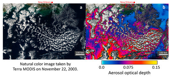
Figure 1.
A sample scene over the Gulf of Mexico just south of New Orleans, illustrating near-cloud aerosol enhancements. (a) Natural color MODIS image; (b) 550 nm aerosol optical depth (AOD) provided for cloud-free areas at 3 km resolution by the MODIS operational Dark Target aerosol product [39,40]. The images are from https://worldview.earthdata.nasa.gov/. The structure of near-cloud areas in parts of this image were analyzed in [38]. High-resolution examples of near-cloud aerosol enhancements observed in 2013 slightly north and west of this scene were shown in [41].
3.1. Dependence on Cloud Properties
In examining how near-cloud aerosol changes depend on the properties of nearby clouds, a critical question is what should be considered a nearby cloud. Cloud identification is an issue because, as put by [42], “the clear-cloudy distinction is ambiguous”, and the distinction used in practice depends both on the scientific context (e.g., what amounts of cloud droplets have negligible effects on the problem being examined) and on the capabilities of observing instruments and data processing methods.
Recognizing the importance of this question, the first step of our analysis is to select the cloud identification criterion that allows us to best separate the clear-sky columns strongly influenced by nearby clouds from those less influenced. Because numerous studies indicated that mean lidar backscatter increases monotonically as we approach clouds [20,21,30,32], we can say that the strongly (less) influenced pixels tend to be closer to (farther from) clouds, respectively. Thus, we can test the performance of various cloud detection criteria by checking which one yields the largest difference between columns closest and farthest from pixels deemed cloudy. Specifically, we consider 5 candidate criteria for identifying a 1 km pixel as cloud: (1) The operational MODIS cloud mask MYD35 [43,44] says “confident cloud”; (2) MODIS operational cloud optical depth (COD) [45] of an overcast or partly cloudy (PCL) pixel exceeds 0; (3) COD of an overcast pixel exceeds 0; (4) COD of an overcast pixel exceeds 1; (5) COD of an overcast pixel exceeds 3.
Figure 2 shows that the difference between near-cloud and far-from-cloud backscatter values is relatively small if we use highly sensitive criteria to detect nearby clouds—namely, MYD35 (which identifies even very thin clouds) or COD + CODPCL > 0 (which identifies even clouds smaller than the 1 km pixel size). This is because using very sensitive criteria puts into the near-cloud category even pixels that are close only to such thin or small clouds that have little impact on their surroundings. As a result, very sensitive criteria are not effective in finding cloud-affected pixels and yield smaller backscatter differences between the near and far categories.
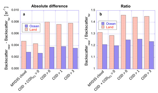
Figure 2.
Differences between mean vertically integrated lidar backscatters of the closer-to-cloud and farther-from-cloud halves of all clear pixels, plotted separately for 5 different criteria used for identifying nearby clouds. (a) Absolute difference; (b) Ratio. MYD35 is the MODIS operational cloud mask, COD and CODPCL are the cloud optical depths of overcast and partly cloudy pixels, respectively. Data used for generating Figure are available at Table S1.
However, Figure 2 also shows that we can better identify pixels affected by cloud-related backscatter enhancements if we use stricter criteria, which put into the near-cloud category only the pixels near “influential” (thick and large) clouds. The figure reveals that once the criteria is sufficiently strict (i.e., clouds are thick enough to allow COD retrievals and large enough to cover a 1 km-size pixel), the exact value of the threshold does not matter much. The rest of this paper will use the COD > 0 criterion to identify nearby clouds, both for consistency with [34], and for the lack of a reason to use a stricter criterion (COD > 1 or 3).
Finally, Figure 2 reveals that for any cloud detection criteria, near-cloud enhancements are significantly stronger over land than over ocean. This is significant because most earlier studies examined near-cloud enhancements over ocean, and the enhancements over land remained largely unknown.
Figure 3a further illustrates that near-cloud enhancements are stronger over land than ocean, and it also shows that vertically integrated backscatter is stronger over land than ocean even quite far from clouds. This is consistent with the mean AOD being higher over land [46] due to the abundance of aerosol sources (e.g., industrial pollution, dust-covered deserts, biomass burning).
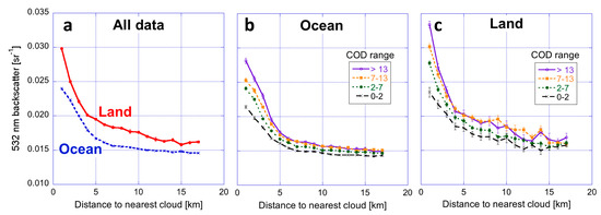
Figure 3.
Mean vertically integrated lidar backscatter, plotted as a function of distance to clouds. (a) All data (Data used are available at Table S2); (b) Data for various ranges of the maximum nearby cloud optical depth (COD) over ocean (Data used are available at Table S3); (c) Same as Panel b, but over land (Data used are available at Table S4). Fraction of used CALIOP columns (in %) that fall into each COD range plotted in Figure 3b,c is available at Table S11.
Figure 3b,c break down the overall behavior seen in Figure 3a into four ranges of the maximum nearby COD (defined as the highest COD observed no more than 2 km farther than the nearest cloud). We note that the same four COD ranges were used by [34], who found stronger enhancements in solar reflectance near thicker clouds. They argued that reflectance enhancements were stronger near thicker clouds at least in part because of stronger three-dimensional (3D) radiative effects (which caused the enhancements to be asymmetric with respect to the solar direction). Figure 3b,c reveal that, despite the absence of 3D effects in lidar backscatter, thicker clouds are associated with larger enhancements within about 5 km from clouds. This may be caused either by thicker clouds containing more droplets (which play key roles in the processing of aerosols through collision/coalescence and in the formation of new aerosol particles [47]), or by thicker clouds being associated with stronger humidity variations (which cause stronger aerosol swelling).
Finally, we note that Figure 3 features visibly larger error bars over land and at larger distances from clouds (where the smaller number of data points causes larger sampling uncertainties), but also that the uncertainties are much smaller than the systematic changes discussed here.
The impact of nearby COD on near-cloud enhancements is explored further in Figure 4. In this figure, near-cloud enhancement is quantified as the difference between the mean vertically integrated lidar backscatters 1–2 km and 10–15 km from clouds. The figure suggests that the enhancements appear to increase roughly as logarithmic functions of COD. This implies that as clouds get thicker, mean near-cloud enhancements increase proportionally to the relative change in COD. For example, a two-fold increase in COD corresponds to a roughly 0.001 increase in mean near-cloud enhancements.
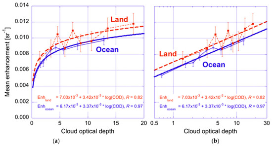
Figure 4.
Mean near-cloud enhancement in vertically integrated lidar backscatter, plotted as a function of maximum cloud optical depth (COD) of nearby clouds. The near-cloud enhancement is calculated as the difference between the mean vertically integrated lidar backscatters 1-2 km and 10-15 km from clouds. The enhancement is plotted for ten 10%-wide percentile ranges of the “nearby cloud” COD distribution (with the leftmost symbol representing the thinnest 10% of clouds, etc.). Thin lines connect the data points, thick lines represent a logarithmic fit to the data. (a) Linear COD scale; (b) Logarithmic COD scale. (Data used are available at Table S5).
Figure 4 also helps better understand why, as Figure 2 and Figure 3a reveled, near-cloud enhancements are stronger over land than over ocean. First, Figure 4b shows that for any given COD, near-cloud enhancement is larger over land than ocean by about 0.0008—that is, by 20% for very thin clouds (COD ≈ 0.5) and by 10% for the much more typical case of COD ≈ 5. This 10–20% difference may be attributed (1) to land regions containing more aerosols and precursor gases that cloud droplets can process, and (2) to the lower background humidity over land, which allows stronger aerosol swelling as relative humidity rises toward the 100% attained at cloud edges. This 10–20% difference in Figure 4, however, explains only about half of the roughly 35% difference between enhancements over land and ocean in Figure 3a. To understand the other half, we point out that in Figure 4, the symbols (for corresponding data percentiles) are at higher COD values (i.e., more to the right) for land than ocean—indicating that the clouds that occur in broken cloud fields are thicker over land than ocean. In fact, the median COD of “nearby clouds” are 6.3 and 3.5 over land and ocean, respectively. This is consistent with all clouds and liquid clouds being thicker over land than over ocean [48,49]. Since, as mentioned above, a doubling of COD increases near-cloud enhancements by 0.001, the impact of land-ocean COD differences is comparable to the 0.0008 difference in Figure 4b. Thus, we can say that the other half of the difference between near-cloud enhancements over land and ocean comes from the combination of (a) enhancements increasing with cloud thickness and (b) nearby clouds being thicker over land than over ocean.
When interpreting the results in Figure 3 and Figure 4, one may wonder whether the key factor in the enhancements being stronger near thicker clouds is the larger COD itself, or the main factor is in fact larger cloud top height (CTH) that tends to go hand-in-hand with the larger COD [49,50]. (For example, as the COD of nearby oceanic clouds increases from 0 to 15, their mean CTH increases from 1.2 km to 2 km. In turn, as the CTH of clouds increases from near 0 to 3 km, their mean COD increases from 2 to 11.) CTH could be an important factor because it indicates the top of the planetary boundary layer, which tends to contain much more aerosol than the free troposphere above. Therefore, given a constant surface elevation (for example over ocean), a higher CTH implies a thicker aerosol-rich boundary layer—and perhaps the swelling of more aerosol particles when humidity increases near clouds.
To see whether COD or CTH has the primary role in near-cloud enhancements, Figure 5a,b split the total data populations into 4 quartiles based on COD or CTH, respectively. (To prevent surface elevation changes from complicating the relationship between CTH and boundary layer thickness, only data over ocean is considered.) The comparison of Panels a and b shows a much wider spread between the curves in Panel a than in Panel b, especially within the first 5 km from clouds. This indicates that COD is a more effective measure than CTH for identifying data points impacted by strong or weak near-cloud enhancements. This implies that COD is the primary factor with a stronger link to near-cloud enhancements. The role of CTH may be limited because even within the boundary layer, aerosol concentrations are largest at the lowest altitudes [51]—and so thickening the boundary layer by raising its top altitude may add only small amounts of aerosols.
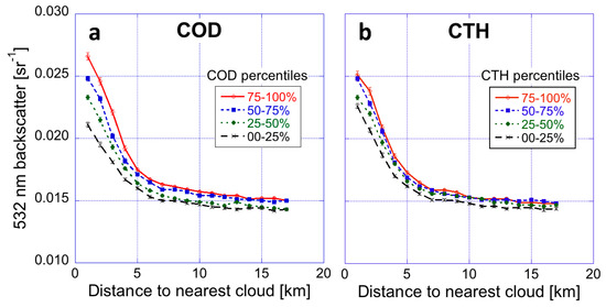
Figure 5.
Mean vertically integrated backscatter, plotted for oceanic areas as a function of distance to the nearest clouds. (a) The dataset is split into 4 quartiles based on the maximum cloud optical depth (COD) of nearby clouds (Data used are available at Table S6); (b) The dataset is split into 4 quartiles based on the maximum cloud top height (CTH) of nearby clouds (Data used are available at Table S7).
3.2. Dependence on Aerosol Type
Naturally, near-cloud enhancements can be suspected to depend on the properties of not only nearby clouds, but also on the properties of aerosols. Therefore, this section explores how the enhancements depend on aerosol type. Following [26], we examine the impact of aerosol type by calculating separate statistics using only the data for which there is a dominant aerosol type: a single aerosol type provides more than 50% of the total AOD in the MERRA-2 global reanalysis.
Figure 6 shows that near-cloud aerosol enhancements are weakest when the aerosol population is dominated by dust. This is likely due to dust particles being weakly hygroscopic, and to dust layers often occurring above the altitude of nearby clouds (where they are not impacted by those clouds [21]). We note that near-cloud enhancements for dust are probably even weaker than it appears in Figure 6, considering that other, more hygroscopic aerosol types can be present at low altitudes even in atmospheric columns dominated by dust.
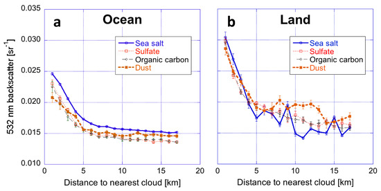
Figure 6.
Mean vertically integrated lidar backscatter for cases dominated by certain aerosol types. Black carbon is not included because it never dominated the aerosol population in our dataset. (a) Data over ocean (Data used are available at Table S8); (b) Data over land (Data used are available at Table S9). Fraction of used CALIOP columns (in %) assigned to each aerosol type in plotting Figure 6 is available at Table S12.
Figure 6 also shows that near-cloud enhancements are strongest for cases dominated by sea salt; their enhancements exceed those of dust-dominated cases by about 50%. This is probably because sea salt is quite hygroscopic and is quite prevalent at low altitudes, where it can be affected by nearby boundary layer clouds and associated humidity increases.
A comparison of Figure 6a,b also shows that the impact of aerosol type on near-cloud enhancements is weaker over land than over ocean, although the large uncertainties over land make it hard to draw very specific conclusions. Over ocean, though, the difference between aerosol types greatly exceeds the level of uncertainty.
3.3. Role of Large-Scale Meteorological Conditions and Processes
In trying to better understand the behaviors discussed above, one may wonder whether in Figure 3, Figure 4, Figure 5 and Figure 6 the mean backscatter values are higher near clouds because of local effects associated with individual clouds, or because of large-scale variations in meteorological conditions such as humidity, aerosol transport, or the intensity of aerosol sources and sinks. For example, large-scale conditions could cause enhanced mean backscatter values within a few km-s from clouds in Figure 3, Figure 4, Figure 5 and Figure 6, if the wind caused by large-scale weather patterns was stronger in partly cloudy regions where clouds tend to be separated by small gaps. The stronger wind could lift more sea salt or dust particles into the atmosphere, thus increasing the backscatter values. Because of the small gaps between clouds, these regions would contain an abundance of near-cloud CALIOP columns. This, in turn, would imply that the global population of all near-cloud columns in Figure 3, Figure 4, Figure 5 and Figure 6 would be heavily influenced by such areas of large backscatter. In contrast, the global population for large distances from clouds would not be influenced by these large-backscatter areas dominated by small gaps between clouds. As a result, wind variations occurring at scales of hundreds of km-s (for example at the scales of entire cloud fields) could conceivably result in higher global mean backscatter values at the first few distance bins (up to about 5–10 km in Figure 3, Figure 4, Figure 5 and Figure 6) than at farther-away bins—even without any local aerosol variations in the vicinity of individual clouds.
We examine the contribution of large-scale meteorological conditions and processes to near-cloud aerosol enhancements by creating a plot similar to Figure 3a, but with one key difference: In processing each point in our dataset, we update the mean value of the appropriate distance-to-cloud bin using not the vertically integrated lidar backscatter of the point, but the MERRA-2 scattering AOD of the 0.5° X 0.625° latitude-longitude area that contains the point.
The mean MERRA-2 AOD values obtained this way help, because MERRA-2 data captures the impact of large-scale (≥50 km) conditions, but not the local variations around individual clouds. Figure 7 shows that the MERRA-2 AOD values, which represent 0.5° X 0.625° areas around each point, do not change systematically with the point’s distance to clouds. This implies that the near-cloud enhancements in Figure 3, Figure 4, Figure 5 and Figure 6 are not caused by near-cloud and far-from-cloud points experiencing systematically different large-scale meteorological conditions. Instead, the enhancements are caused predominantly by local variations around individual clouds (see Figure 1 for examples).
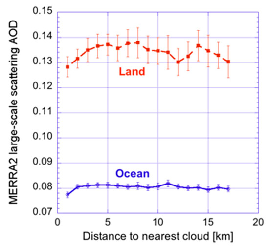
Figure 7.
Mean AOD provided by the MERRA-2 global reanalysis for large regions that surround points located at certain distances from nearby clouds. See text for details. (Data used are available at Table S10).
We note that large-scale conditions not being responsible for the higher backscatter values near clouds is consistent with the finding of [52], that large-scale variations in cloud cover contribute little to backscatter being higher near clouds. In contrast, [53] found that variations in cloud cover did strengthen near-cloud enhancements—perhaps because their dataset included seasonal variations as well. We point out, however, that while [52] and [53] examined only one large-scale meteorological factor (cloud cover) in relatively small regions of the northeast Atlantic Ocean, the new results represent the entire globe and consider all large-scale meteorological factors and processes included in MERRA-2 (e.g., cloud cover, humidity, wind, or aerosol transport/sinks/sources).
4. Conclusions
This study explored an important aspect of aerosol-cloud interactions, the impact of clouds and cloud-related processes on nearby aerosols. This topic has attracted wide interest from the community because numerous earlier studies found that clouds and cloud-related processes have a strong influence on the physical and chemical properties of atmospheric aerosols and on our estimates of direct and indirect aerosol radiative effects.
This study sought new insights from a statistical analysis of a global dataset comprising MODIS and CALIOP satellite observations and MERRA-2 reanalysis. The dataset covered June, July and August of 2012, 2013, and 2014, and the analysis focused on aerosols near low clouds. Analyzing the dataset, the paper examined how cloud-related enhancements in lidar backscatter vary with the underlying surface type (land vs. ocean), with the size, altitude, and optical depth of nearby clouds, and with the type of aerosol particles. It also examined whether cloud-related enhancements can be attributed to large-scale meteorological effects, or to local variability around individual clouds.
Earlier studies examined aerosol enhancements mostly over ocean; the new results revealed that near-cloud enhancements over land are even stronger by about 35% (Figure 3). Roughly half of the land-ocean difference was attributed to clouds being thicker over land; reasons for the other half may include differences in humidity and aerosol loading.
The results also indicated that in characterizing the enhancements, it is best to focus on clouds larger than 1 km horizontally, as smaller clouds have a weak impact on their surroundings (Figure 2). Moreover, the results imply that the cloud parameter that impacts aerosol enhancements the most is the optical depth of nearby boundary layer clouds; the altitude of these clouds (and the thickness of the planetary boundary layer) play a secondary role (Figure 5). Moreover, the results showed that aerosol enhancements increase substantially with the optical depth of nearby clouds (COD), and that the rate of increase is roughly proportional to the relative increase in COD (Figure 4). This implies that analyses of cloud-related aerosol enhancement can be greatly improved if we consider not only the distance, but also the optical depth of nearby clouds.
The results also showed that near-cloud enhancements also vary with aerosol type and are about 50% stronger when the majority of the aerosol optical depth is due to sea salt rather than dust (Figure 6). This difference likely comes from the differences discussed in [26,32]: sea salt particles being more hygroscopic, and dust plumes often occurring at higher altitudes where they are not impacted by low-level clouds.
Finally, the study found that the mean lidar backscatter is higher near clouds not because of large-scale variations in meteorological conditions such as humidity, wind, or aerosol transport, but because of local processes associated with the individual clouds nearby (Figure 7). This implies that to accurately account for cloud-related aerosol variations in general circulation models (GCMs), these models need to consider not only the mean parameters of each grid box, but also the subgrid variability associated with unresolved clouds.
Overall, the study characterized multiple aspects of cloud-related variations in aerosol populations. Such information can not only help improve our understanding of aerosol-cloud interactions and aerosol direct and indirect radiative effects, but—ultimately—can help better represent them in GCMs and other atmospheric models.
Supplementary Materials
The following are available online at https://www.mdpi.com/2072-4292/13/6/1151/s1, Table S1: Data values used in creating Figure 2, Table S2: Data values used in creating Figure 3a, Table S3: Data values used in creating Figure 3b, Table S4: Data values used in creating Figure 3c, Table S5: Data values used in creating Figure 4, Table S6: Data values used in creating Figure 5a, Table S7: Data values used in creating Figure 5b, Table S8: Data values used in creating Figure 6a, Table S9: Data values used in creating Figure 6b, Table S10: Data values used in creating Figure 7, Table S11: Fraction of used CALIOP columns (in %) that fall into each COD range plotted in Figure 3b,c, Table S12: Fraction of used CALIOP columns (in %) assigned to each aerosol type in plotting Figure 6.
Author Contributions
Conceptualization, T.V. and A.M.; methodology, T.V.; software, T.V.; validation, A.M and T.V.; formal analysis, T.V.; investigation, T.V.; resources, A.M. and T.V.; data curation, T.V.; writing—original draft preparation, T.V.; writing—review and editing, A.M.; visualization, T.V.; supervision, A.M.; project administration, T.V. and A.M.; funding acquisition, T.V and A.M. Both authors have read and agreed to the published version of the manuscript.
Funding
This research was funded by the NASA Radiation Sciences Program managed by Hal Maring and by the NASA CALIPSO project supervised by David Considine.
Acknowledgments
We are grateful to Ralph Kahn and to Lazaros Oreopoulos for helpful questions and suggestions.
Conflicts of Interest
The authors declare no conflict of interest. The funders had no role in the design of the study; in the collection, analyses, or interpretation of data; in the writing of the manuscript, or in the decision to publish the results.
References
- IPCC. Climate Change 2013: The Physical Science Basis. Contribution of Working Group I to the Fifth Assessment Report of the Intergovernmental Panel on Climate Change; Stocker, T.F., Qin, D., Plattner, G.-K., Tignor, M., Allen, S.K., Boschung, J., Nauels, A., Xia, Y., Bex, V., Midgley, P.M., Eds.; Cambridge University Press: Cambridge, UK; New York, NY, USA, 2013; 1535p. [Google Scholar]
- Eck, T.F.; Holben, B.N.; Reid, J.S.; Giles, D.M.; Rivas, M.A.; Singh, R.P.; Tripathi, S.N.; Bruegge, C.J.; Platnick, S.; Arnold, G.T.; et al. Fog- and cloud-induced aerosol modification observed by the Aerosol Robotic Network (AERONET). J. Geophys. Res. 2012, 117, D07206. [Google Scholar] [CrossRef]
- Eck, T.F.; Holben, B.N.; Reid, J.S.; Arola, A.; Ferrare, R.A.; Hostetler, C.A.; Crumeyrolle, S.N.; Berkoff, T.A.; Welton, E.J.; Lolli, S.; et al. Observations of rapid aerosol optical depth enhancements in the vicinity of polluted cumulus clouds. Atmos. Chem. Phys. 2014, 14, 11633–11656. [Google Scholar] [CrossRef]
- Koren, I.; Feingold, G.; Jiang, H.; Altaratz, O. Aerosol effects on the inter-cloud region of a small cumulus cloud field. Geophys. Res. Lett. 2009, 36, L14805. [Google Scholar] [CrossRef]
- Bar-Or, R.Z.; Koren, I.; Altaratz, O.; Fredj, E. Radiative properties of humidified aerosols in cloudy environment. Atmos. Res. 2012, 118, 280–294. [Google Scholar] [CrossRef]
- Jeong, M.J.; Li, Z. Separating real and apparent effects of cloud, humidity, and dynamics on aerosol optical thickness near cloud edges. J. Geophys. Res. 2010, 115, D00K32. [Google Scholar] [CrossRef]
- Chand, D.; Wood, R.; Ghan, S.; Wang, M.; Ovchinnikov, M.; Rasch, P.J.; Miller, S.; Schichtel, B.; Moore, T. Aerosol optical depth enhancement in partly cloudy conditions. J. Geophys. Res. 2012, 117, D17207. [Google Scholar]
- Arola, A.; Eck, T.F.; Kokkola, H.; Pitkänen, M.R.A.; Romakkaniemi, S. Assessment of cloud-related fine-mode AOD enhancements based on AERONET SDA product. Atmos. Chem. Phys. 2017, 17, 5991–6001. [Google Scholar] [CrossRef]
- Eck, T.F.; Holben, B.N.; Reid, J.S.; Xian, P.; Giles, D.M.; Sinyuk, A.; Smirnov, A.; Schafer, J.S.; Slutsker, I.; Kim, J.; et al. Observations of the interaction and transport of fine mode aerosols with cloud and/or fog in Northeast Asia from Aerosol Robotic Network and satellite remote sensing. J. Geophys. Res. 2018, 123, 5560–5587. [Google Scholar] [CrossRef] [PubMed]
- Twohy, C.H.; Coakley, J.A., Jr.; Tahnk, W.R. Effect of changes in relative humidity on aerosol scattering near clouds. J. Geophys. Res. 2009, 114, D05205. [Google Scholar] [CrossRef]
- Rauber, R.M.; Zhao, G.; Di Girolamo, L.; Colón-Robles, M. Aerosol size distribution, particle concentration, and optical property variability near Caribbean trade cumulus clouds: Isolating effects of vertical transport and cloud processing from humidification using aircraft measurements. J. Atmos. Sci. 2013, 70, 3063–3083. [Google Scholar] [CrossRef]
- Hudson, J.G.; Noble, S.; Tabor, S. Cloud supersaturations from CCN spectra Hoppel minima. J. Geophys. Res. 2015, 120, 3436–3452. [Google Scholar] [CrossRef]
- Ignatov, A.; Minnis, P.; Loeb, N.G.; Wielicki, B.; Miller, W.; Sun-Mack, S.; Tanré, D.; Remer, L.; László, I.; Geier, E. Two MODIS aerosol products over ocean on the Terra and Aqua CERES SSF. J. Atmos. Sci. 2005, 62, 1008–1031. [Google Scholar] [CrossRef]
- Loeb, N.G.; Manalo-Smith, N. Top-of-Atmosphere direct radiative effect of aerosols over global oceans from merged CERES and MODIS observations. J. Clim. 2005, 18, 3506–3526. [Google Scholar] [CrossRef]
- Zhang, J.; Reid, J.S.; Holben, B.N. An analysis of potential cloud artifacts in MODIS over ocean aerosol optical thickness products. Geophys. Res. Lett. 2005, 32, L15803. [Google Scholar] [CrossRef]
- Loeb, N.G.; Schuster, G.L. An observational study of the relationship between cloud, aerosol and meteorology in broken low-level cloud conditions. J. Geophys. Res. 2008, 113, D14214. [Google Scholar] [CrossRef]
- Koren, I.; Remer, L.A.; Kaufman, Y.J.; Rudich, Y.; Martins, J.V. On the twilight zone between clouds and aerosols. Geophys. Res. Lett. 2007, 34, L08805. [Google Scholar] [CrossRef]
- Su, W.; Schuster, G.L.; Loeb, N.G.; Rogers, R.R.; Ferrare, R.A.; Hostetler, C.A.; Hair, J.W.; Obland, M.D. Aerosol and cloud interaction observed from high spectral resolution lidar data. J. Geophys. Res. 2008, 113, D24202. [Google Scholar] [CrossRef]
- Redemann, J.; Zhang, Q.; Russell, P.B.; Livingston, J.M.; Remer, L.A. Case studies of aerosol remote sensing in the vicinity of clouds. J. Geophys. Res. 2009, 114, D6. [Google Scholar] [CrossRef]
- Tackett, J.L.; Di Girolamo, L. Enhanced aerosol backscatter adjacent to tropical trade wind clouds revealed by satellite-based lidar. Geophys. Res. Lett. 2009, 36, L14804. [Google Scholar] [CrossRef]
- Várnai, T.; Marshak, A. Global CALIPSO observations of aerosol changes near clouds. IEEE Geosci. Remote Sens. Lett. 2011, 8, 19–23. [Google Scholar] [CrossRef]
- Várnai, T.; Marshak, A. Satellite observations of cloud-related variations in aerosol oroperties. Atmosphere 2018, 9, 430. [Google Scholar] [CrossRef]
- Konwar, M.; Panicker, A.S.; Axisa, D.; Prabha, T.V. Near-cloud aerosols in monsoon environment and its impact on radiative forcing. J. Geophys. Res. 2015, 120, 1445–1457. [Google Scholar] [CrossRef]
- Christensen, M.W.; Neubauer, D.; Poulsen, C.A.; Thomas, G.E.; McGarragh, G.R.; Povey, A.C.; Proud, S.R.; Grainger, R.G. Unveiling aerosol–cloud interactions—Part 1: Cloud contamination in satellite products enhances the aerosol indirect forcing estimate. Atmos. Chem. Phys. 2017, 17, 13151–13164. [Google Scholar] [CrossRef]
- Liu, J.; Li, Z. Significant underestimation in the optically based estimation of the aerosol first indirect effect induced by the aerosol swelling effect. Geophys. Res. Lett. 2018, 45, 5690–5699. [Google Scholar] [CrossRef]
- Várnai, T.; Marshak, A.; Eck, T.F. Observation-based study on aerosol optical depth and particle size in partly cloudy regions. J. Geophys. Res. 2017, 122, 10013–10024. [Google Scholar] [CrossRef] [PubMed]
- Winker, D.M.; Pelon, J.; Coakley, J.A., Jr.; Ackerman, S.A.; Charlson, R.J.; Colarco, P.R.; Flamant, P.; Fu, Q.; Hoff, R.M.; Kittaka, C.; et al. The CALIPSO mission: A global 3D view of aerosols and clouds. Bull. Am. Meteorol. Soc. 2010, 91, 1211–1230. [Google Scholar] [CrossRef]
- Salomonson, V.V.; Barnes, W.L.; Maymon, P.W.; Montgomery, H.E.; Ostrow, H. MODIS: Advanced facility instrument for studies of the Earth as a system. IEEE Trans. Geosci. Remote Sens. 1989, 27, 145–153. [Google Scholar] [CrossRef]
- Gelaro, R.; McCarty, W.; Suárez, M.J.; Todling, R.; Molod, A.; Takacs, L.; Randles, C.A.; Darmenov, A.; Bosilovich, M.G.; Reichle, R.; et al. The Modern-Era Retrospective Analysis for Research and Applications, Version 2 (MERRA-2). J. Clim. 2017, 30, 5419–5454. [Google Scholar] [CrossRef]
- Yang, W.; Marshak, A.; Várnai, T.; Kalashnikova, O.V.; Kostinski, A.B. CALIPSO observations of transatlantic dust: Vertical stratification and effect of clouds. Atmos. Chem. Phys. 2012, 12, 11339–11354. [Google Scholar] [CrossRef]
- Yang, W.; Marshak, A.; Várnai, T.; Liu, S. Effect of CALIPSO cloud–aerosol discrimination (CAD) confidence levels on observations of aerosol properties near clouds. Atmos. Res. 2012, 116, 134–141. [Google Scholar] [CrossRef]
- Várnai, T.; Marshak, A.; Yang, W. Multi-satellite aerosol observations in the vicinity of clouds. Atmos. Chem. Phys. 2013, 13, 3899–3908. [Google Scholar] [CrossRef]
- Wen, G.; Marshak, A.; Cahalan, R.F.; Remer, L.A.; Kleidman, R.G. 3D aerosol-cloud radiative interaction observed in collocated MODIS and ASTER images of cumulus cloud fields. J. Geophys. Res. 2007, 112, D13204. [Google Scholar] [CrossRef]
- Várnai, T.; Marshak, A. MODIS observations of enhanced clear sky reflectance near clouds. Geophys. Res. Lett. 2009, 36, L06807. [Google Scholar] [CrossRef]
- Stap, F.A.; Hasekamp, O.P.; Emde, C.; Röckmann, T. Multiangle photopolarimetric aerosol retrievals in the vicinity of clouds: Synthetic study based on a large eddy simulation. J. Geophys. Res. 2016, 121, 12914–12935. [Google Scholar] [CrossRef]
- Vaughan, M.A.; Powell, K.A.; Winker, D.M.; Hostetler, C.A.; Kuehn, R.E.; Hunt, W.H.; Getzewich, B.J.; Young, S.A.; Liu, Z.; McGill, M.J. Fully automated detection of cloud and aerosol layers in the CALIPSO lidar measurements. J. Atmos. Oceanic Tech. 2009, 26, 2034–2050. [Google Scholar] [CrossRef]
- Chin, M. Ginoux, P.; Kinne, S.; Torres, O.; Holben, B.N.; Duncan, B.N.; Marin, R.V.; Logan, J.A.; Higurashi, A.; Nakajima, T. Tropospheric aerosol optical thickness from the GOCART model and comparisons with satellite and sun photometer measurements. J. Atmos. Sci. 2002, 59, 461–483. [Google Scholar] [CrossRef]
- Várnai, T.; Marshak, A. Analysis of co-located MODIS and CALIPSO observations near clouds. Atmos. Meas. Tech. 2012, 5, 389–396. [Google Scholar] [CrossRef]
- Remer, L.A.; Kaufman, Y.J.; Tanre, D.; Mattoo, S.; Chu, D.A.; Martins, J.V.; Li, R.R.; Ichoku, C.; Levy, R.C.; Kleidman, R.G.; et al. The MODIS aerosol algorithm, products, and validation. J. Atmos. Sci. 2005, 62, 947–973. [Google Scholar] [CrossRef]
- Levy, R.C.; Mattoo, S.; Munchak, L.A.; Remer, L.A.; Sayer, A.M.; Patadia, F.; Hsu, N.C. The Collection 6 MODIS aerosol products over land and ocean. Atmos. Meas. Tech. 2013, 6, 2989–3034. [Google Scholar] [CrossRef]
- Spencer, R.S.; Levy, R.C.; Remer, L.A.; Mattoo, S.; Arnold, G.T.; Hlavka, D.L.; Meyer, K.G.; Marshak, A.; Wilcox, E.M.; Platnick, S.E. Exploring aerosols near clouds with high-spatial-resolution aircraft remote sensing during SEAC4RS. J. Geophys. Res. 2019, 124, 2148–2173. [Google Scholar] [CrossRef]
- Charlson, R.; Ackerman, A.; Bender, F.; Anderson, T.; Liu, Z. On the climate forcing consequences of the albedo continuum between cloudy and clear air. Tellus 2007, 59, 715–727. [Google Scholar] [CrossRef]
- Frey, R.A.; Ackerman, S.A.; Liu, Y.H.; Strabala, K.I.; Zhang, H.; Key, J.R.; Wang, X.G. Cloud detection with MODIS. Part I: Improvements in the MODIS cloud mask for collection 5. J. Atmos. Ocean. Technol. 2008, 25, 1057–1072. [Google Scholar] [CrossRef]
- Ackerman, S.A.; Holz, R.E.; Frey, R.; Eloranta, E.W.; Maddux, B.C.; McGill, M. Cloud detection with MODIS. Part II: Validation. J. Atmos. Ocean. Technol. 2008, 25, 1073–1086. [Google Scholar] [CrossRef]
- Platnick, S.; Meyer, K.; King, M.D.; Wind, G.; Amarasinghe, N.; Marchant, B.; Arnold, G.T.; Zhang, Z.; Hubanks, P.A.; Holz, R.E.; et al. The MODIS cloud optical and microphysical products: Collection 6 updates and examples from Terra and Aqua. IEEE Trans. Geosci. Remote Sens. 2017, 55, 502–525. [Google Scholar] [CrossRef] [PubMed]
- Remer, L.A.; Kleidman, R.G.; Levy, R.C.; Kaufman, Y.J.; Tanré, D.; Mattoo, S.; Martins, J.V.; Ichoku, C.; Koren, I.; Yu, H.; et al. Global aerosol climatology from the MODIS satellite sensors. J. Geophys. Res. 2008, 113, D14S07. [Google Scholar] [CrossRef]
- Ervens, B. Turpin, B.J.; Weber, R.J. Secondary organic aerosol formation in cloud droplets and aqueous particles (aqSOA): A review of laboratory, field and model studies. Atmos. Chem. Phys. 2011, 11, 11069–11102. [Google Scholar] [CrossRef]
- Yu, H.; Kaufman, Y.J.; Chin, M.; Feingold, G.; Remer, L.A.; Anderson, T.L.; Balkanski, Y.; Bellouin, N.; Boucher, O.; Christopher, S.; et al. A review of measurement-based assessments of the aerosol direct radiative effect and forcing. Atmos. Chem. Phys. 2006, 6, 613–666. [Google Scholar] [CrossRef]
- King, M.D.; Platnick, S.; Menzel, W.P.; Ackerman, S.A.; Hubanks, P.A. Spatial and temporal distribution of clouds observed by MODIS onboard the Terra and Aqua satellites. IEEE Trans. Geosci. Remote Sens. 2013, 51, 3826–3852. [Google Scholar] [CrossRef]
- Marchand, R.; Ackerman, T.; Smyth, M.; Rossow, W.B. A review of cloud top height and optical depth histograms from MISR, ISCCP, and MODIS. J. Geophys. Res. 2010, 115, D16206. [Google Scholar] [CrossRef]
- Koffi, B.; Schulz, M.; Bréon, F.M.; Dentener, F.; Steensen, B.M.; Griesfeller, J.; Winker, D.; Balkanski, Y.; Bauer, S.E.; Bellouin, N.; et al. Evaluation of the aerosol vertical distribution in global aerosol models through comparison against CALIOP measurements: AeroCom phase II results. J. Geophys. Res. 2016, 121, 7254–7283. [Google Scholar] [CrossRef] [PubMed]
- Várnai, T.; Marshak, A. Effect of cloud fraction on near-cloud aerosol behavior in the MODIS atmospheric correction ocean color product. Remote Sens. 2015, 7, 5283–5299. [Google Scholar] [CrossRef]
- Yang, W.; Marshak, A.; Várnai, T.; Wood, R. CALIPSO observations of near-cloud aerosol properties as a function of cloud fraction. Geophys. Res. Lett. 2014, 41, 9150–9157. [Google Scholar] [CrossRef]


Publisher’s Note: MDPI stays neutral with regard to jurisdictional claims in published maps and institutional affiliations. |
© 2021 by the authors. Licensee MDPI, Basel, Switzerland. This article is an open access article distributed under the terms and conditions of the Creative Commons Attribution (CC BY) license (http://creativecommons.org/licenses/by/4.0/).