
Determining the Intangible: Detecting Land Abandonment at Local Scale


Abstract
:
1. Introduction
2. Materials and Methods
3. Results
4. Discussion
5. Conclusions
Author Contributions
Funding
Institutional Review Board Statement
Informed Consent Statement
Data Availability Statement
Conflicts of Interest
References
- De Amorim, W.S.; Borchardt Deggau, A.; do Livramento Gonçalves, G.; da Silva Neiva, S.; Prasath, A.R.; Salgueirinho Osório de Andrade Guerra, J.B. Urban challenges and opportunities to promote sustainable food security through smart cities and the 4th industrial revolution. Land Use Policy 2019, 87, 104065. [Google Scholar] [CrossRef]
- World Economic Forum. Global Risks Report 2019; World Economic Forum: Geneva, Switzerland, 2019; ISBN 9781944835156. [Google Scholar]
- De Amorim, W.S.; Valduga, I.B.; Ribeiro, J.M.P.; Williamson, V.G.; Krauser, G.E.; Magtoto, M.K.; de Andrade Guerra, J.B.S.O. The nexus between water, energy, and food in the context of the global risks: An analysis of the interactions between food, water, and energy security. Environ. Impact Assess. Rev. 2018, 72, 1–11. [Google Scholar] [CrossRef]
- Piniero, M.-C. Globalization and industrialization of agriculture: Impacts on rural Chocontá, Colombia. Luna Azul 2016, 43, 468–498. [Google Scholar] [CrossRef] [Green Version]
- Marsden, T. Mobilities, vulnerabilities and sustainabilities: Exploring pathways from denial to sustainable rural development. Sociol. Rural. 2009, 49, 113–131. [Google Scholar] [CrossRef]
- Azhar, B.; Lindenmayer, D.B.; Wood, J.; Fischer, J.; Zakaria, M. Ecological impacts of oil palm agriculture on forest mammals in plantation estates and smallholdings. Biodivers. Conserv. 2014, 23, 1175–1191. [Google Scholar] [CrossRef]
- Alcantara, C.; Kuemmerle, T.; Prishchepov, A.V.; Radeloff, V.C. Mapping abandoned agriculture with multi-temporal MODIS satellite data. Remote Sens. Environ. 2012, 124, 334–347. [Google Scholar] [CrossRef]
- Li, S.; Li, X. Global understanding of farmland abandonment: A review and prospects. J. Geogr. Sci. 2017, 27, 1123–1150. [Google Scholar] [CrossRef]
- Queiroz, C.; Beilin, R.; Folke, C.; Lindborg, R. Farmland abandonment: Threat or opportunity for biodiversity conservation? A global review. Front. Ecol. Environ. 2014, 12, 288–296. [Google Scholar] [CrossRef]
- Ramankutty, N.; Foley, J.A. Estimating historical changes in land cover North American croplands from 1850 to 1992. Glob. Ecol. Biogeogr. 1999, 8, 381–396. [Google Scholar] [CrossRef]
- MacDonald, D.; Crabtree, J.R.; Wiesinger, G.; Dax, T.; Stamou, N.; Fleury, P.; Gutierrez Lazpita, J.; Gibon, A. Agricultural abandonment in mountain areas of Europe: Environmental consequences and policy response. J. Environ. Manag. 2000, 59, 47–69. [Google Scholar] [CrossRef]
- Savulescu, I.; Mihai, B.A.; Vîrghileanu, M.; Nistor, C.; Olariu, B. Mountain arable land abandonment (1968–2018) in the Romanian Carpathians: Environmental conflicts and sustainability issues. Sustainability 2019, 11, 6679. [Google Scholar] [CrossRef] [Green Version]
- Janus, J.; Bozek, P. Land abandonment in Poland after the collapse of socialism: Over a quarter of a century of increasing tree cover on agricultural land. Ecol. Eng. 2019, 138, 106–117. [Google Scholar] [CrossRef]
- Kolecka, N.; Kozak, J.; Kaim, D.; Dobosz, M.; Ostafin, K.; Ostapowicz, K.; Wężyk, P.; Price, B. Understanding farmland abandonment in the Polish Carpathians. Appl. Geogr. 2017, 88, 62–72. [Google Scholar] [CrossRef]
- Corbelle Rico, E.; Crecente Maseda, R. Land Abandonment Concept and Consequences. Rev. Galega Econ. 2008, 17, 1–13. [Google Scholar]
- Keenleyside, C.; Tucker, G. Farmland Abandonment in the EU: An Assessment of Trends and Prospects; Report prepared for WWF; Institute for European Environmental Policy: London, UK, 2010. [Google Scholar]
- Gałecka-Drozda, A.; Zachariasz, A. Tereny postagrarne w największych miastach Polski. Pr. Kom. Kraj. Kult. Cult. Landsc. Comm. 2017, 38, 57–70. [Google Scholar]
- FAO FAOSTAT. Methods & Standards. Available online: http://www.fao.org/ag/agn/nutrition/Indicatorsfiles/Agriculture.pdf (accessed on 30 June 2020).
- Krysiak, S. Odłogi w krajobrazach Polski środkowej—Aspekty przestrzenne, typologiczne i ekologiczne. Probl. Ekol. Kraj. 2011, 41, 89–96. [Google Scholar]
- Cocca, G.; Sturaro, E.; Gallo, L.; Ramanzin, M. Is the abandonment of traditional livestock farming systems the main driver of mountain landscape change in Alpine areas? Land Use Policy 2012, 29, 878–886. [Google Scholar] [CrossRef]
- Pointereau, P.; Coulon, F.; Girard, P.; Lambotte, M.; Stuczynski, T.; Sánchez Ortega, V.; Del Rio, A. Analysis of Farmland Abandonment and the Extent and Location of Agricultural Areas that are Actually Abandoned or are in Risk to be Abandoned; Anguiano, E., Bamps, C., Terres, J., Red, M., Eds.; European Commission Joint Research Centre: Brussels, Belgium, 2008; ISBN EUR 23411EN. [Google Scholar]
- Rey Benayas, J.; Matins, A.; Nicolau, J.M.; Schulz, J.J. Abandonment of agricultural land: An overview of drivers and consequences. CAB Rev. Perspect. Agric. Vet. Sci. Nutr. Nat. Resour. 2007, 2, 1–14. [Google Scholar] [CrossRef] [Green Version]
- Ruppert, K. Zur Definition des Begriffes “Sozialbrache” (The Meaning of the Term “Sozialbrache” (Social Fallow)). Erdkunde 1958, 12, 226–231. [Google Scholar]
- Terres, J.M.; Scacchiafichi, L.N.; Wania, A.; Ambar, M.; Anguiano, E.; Buckwell, A.; Coppola, A.; Gocht, A.; Källström, H.N.; Pointereau, P.; et al. Farmland abandonment in Europe: Identification of drivers and indicators, and development of a composite indicator of risk. Land Use Policy 2015, 49, 20–34. [Google Scholar] [CrossRef]
- Satola, L.; Wojewodzic, T.; Sroka, W. Barriers to exit encountered by small farms in light of the theory of new institutional economics. Agric. Econ. 2018, 64, 277–290. [Google Scholar]
- Wojewodzic, T. Procesy Dywestycji i Dezagraryzacji w Rolnictwie na Obszarach o Rozdrobnionej Strukturze Agrarnej. In Zeszyty Naukowe Uniwersytetu Rolniczego; Wydawnictwo Uniwersytetu Rolniczego: Kraków, Poland, 2017. [Google Scholar]
- Perpiña Castillo, C.; Kavalov, B.; Diogo, V.; Jacobs-Crisioni, C.; Batista e Silva, F.; Lavalle, C. JRC Policy Insights: Agricultural Land Abandonment in the EU within 2015–2030; JRC Working Papers JRC113718; Joint Research Centre (Seville site): Ispra, Italy, 2018; pp. 1–7. [Google Scholar]
- Rola, J.; Rola, H. Solidago SPP. biowskaźnikiem występowania odłogów na gruntach rolnych. Fragm. Agron. 2010, 27, 122–131. [Google Scholar]
- Schneeberger, N.; Bürgi, M.; Kienast, P.D.F. Rates of landscape change at the northern fringe of the Swiss Alps: Historical and recent tendencies. Landsc. Urban Plan. 2007, 80, 127–136. [Google Scholar] [CrossRef]
- Bieling, C.; Plieninger, T.; Schaich, H. Patterns and causes of land change: Empirical results and conceptual considerations derived from a case study in the Swabian Alb, Germany. Land Use Policy 2013, 35, 192–203. [Google Scholar] [CrossRef]
- Witmer, F.D.W.; O’Loughlin, J. Satellite Data Methods and Application in the Evaluation of War Outcomes: Abandoned Agricultural Land in Bosnia-Herzegovina After the 1992–1995 Conflict. Ann. Assoc. Am. Geogr. 2009, 99, 1033–1044. [Google Scholar] [CrossRef]
- Alcantara, C.; Kuemmerle, T.; Baumann, M.; Bragina, E.V.; Griffiths, P.; Hostert, P.; Knorn, J.; Müller, D.; Prishchepov, A.V.; Schierhorn, F.; et al. Mapping the extent of abandoned farmland in Central and Eastern Europe using MODIS time series satellite data. Environ. Res. Lett. 2013, 8, 035035. [Google Scholar] [CrossRef]
- Prishchepov, A.V.; Radeloff, V.C.; Dubinin, M.; Alcantara, C. The effect of Landsat ETM/ETM+ image acquisition dates on the detection of agricultural land abandonment in Eastern Europe. Remote Sens. Environ. 2012, 126, 195–209. [Google Scholar] [CrossRef]
- Majchrowska, A. Abandonment of agricultural land in central Poland and its ecological role. Ekológia 2013, 32, 320–327. [Google Scholar] [CrossRef]
- Czesak, B.; Cegielska, K.; Cherkes, B.; Różycka-Czas, R.; Salata, T. Fieldwork approach to determining the extent of agricultural land abandonment-case study. Geomat. Landmanag. Landsc. 2016, 3, 21–31. [Google Scholar] [CrossRef]
- Ministerstwo Rolnictwa i Rozwoju Wsi. Diagnoza Sutuacji Społęczno-Gospodarczej Rolnictwa, Obszarów Wiejskich i Rybactwa w Polscie; Ministerstwo Rolnictwa i Rozwoju Wsi: Warszawa, Poland, 2019.
- Janus, J.; Taszakowski, J. The Idea of Ranking in Setting Priorities for Land Consolidation Works. Geomat. Landmanag. Landsc. 2015, 1, 31–43. [Google Scholar] [CrossRef]
- Janus, J.; Glowacka, A.; Bozek, P. Identification of Areas With Unfavorable Agriculture Development. Eng. Rural Dev. 2016, 1260–1265. [Google Scholar]
- Król, Ż. Charakterystyka szachownicy gruntów o układzie wstęgowym na przykładzie miejscowości Brzeziny Gmina Puchaczów. Infrastrukt. Ekol. Teren. Wiej. 2014, II, 423–435. [Google Scholar]
- Directive 2007/60/EC of the European Parliament and of the Council of 23 October 2007 on the Assessment and Management of Flood Risks. Available online: https://eur-lex.europa.eu/LexUriServ/LexUriServ.do?uri=OJ:L:2007:288:0027:0034:EN:PDF (accessed on 30 June 2020).
- Wężyk, P. (Ed.) Podręcznik dla Uczestników Szkoleń z Wykorzystania Produktów LiDAR; Główny Urząd Geodezji i Kartografii: Warszawa, Poland, 2015; ISBN 9788325421007. [Google Scholar]
- Szostak, M.; Wężyk, P.; Tompalski, P. Aerial Orthophoto and Airborne Laser Scanning as Monitoring Tools for Land Cover Dynamics: A Case Study from the Milicz Forest District (Poland). Pure Appl. Geophys. 2013, 171, 857–866. [Google Scholar] [CrossRef] [Green Version]
- Łukasik, S. Identyfikacja rozkładu w systemach rzeczywistych za pomocą estymatorów jądrowych. Czas. Tech. Wydaw. Politech. Krakowiskiej 2008, 1, 1–12. [Google Scholar]
- Noszczyk, T.; Hernik, J. Kompleksowa modernizacja ewidencji gruntów i budynków. Acta Sci. Pol. Form. Circumiectus 2016, 15, 3–17. [Google Scholar] [CrossRef]
- Kolecka, N.; Kozak, J. Wall-to-Wall parcel-level mapping of agricultural land abandonment in the Polish Carpathians. Land 2019, 8, 129. [Google Scholar] [CrossRef] [Green Version]
- Tasser, E.; Walde, J.; Tappeiner, U.; Teutsch, A.; Noggler, W. Land-use changes and natural reforestation in the Eastern Central Alps. Agric. Ecosyst. Environ. 2007, 118, 115–129. [Google Scholar] [CrossRef]
- Jucha, W.; Marszałek, A. Zastosowanie danych ALS do interpretacji dawnych i współczesnych form użytkowania terenu na przykładzie wzgórza Grojec. Rocz. Geomatyki 2016, 14, 465–476. [Google Scholar]
- Krysiak, S.; Papińska, E.; Majchrowska, A.; Adamiak, M.; Koziarkiewicz, M. Detecting Land Abandonment in Lodz Voivodeship Using Convolutional Neural Networks. Land 2020, 9, 82. [Google Scholar] [CrossRef] [Green Version]
- Kujawa, A.; Chmielowiec-tyszko, D. Zadrzewienia na Obszarach Wiejskich—Dobre Praktyki i Rekomendacje. 2019. Available online: http://drzewa.org.pl/wp-content/uploads/2018/10/Zadrzewienia-na-obszarach-wiejskich_draft.pdf (accessed on 30 June 2020).
- Scott, P.R.; Branch, R.; Division, P.I. The Role of Trees in Sustainable Agriculture A National Conference Resource Management Technical Report No. 138 Prepared for the National Land and Water Resource Audit; Department of Agriculture and Food: Western Australia, 1992.
- Baumhardt, R.L.; Blanco-Canqui, H. Soil: Conservation Practices. Encycl. Agric. Food Syst. 2014, 153–165. [Google Scholar]
- Rega, C. Ecological Rationality in Spatial Planning Concepts and Tools for Sustainable Land-Use Decisions; Springer: Cham, Switzerland, 2020. [Google Scholar]

| ID | Kernel | Radius | Weight | Coefficient of Variation |
|---|---|---|---|---|
| 1 | Epanechnikov | 5 | - | 1.29 |
| 2 | triweight | 5 | - | 0.77 |
| 3 | Epanechnikov | 5 | class of height | 1.3 |
| 4 | triweight | 5 | class of height | 0.85 |
| 5 | Epanechnikov | class of height | - | 1.1 |
| 6 | triweight | class of height | - | 0.92 |
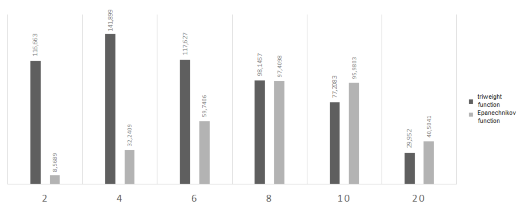
| ID | Kernel | Isoline | Sum of Surface Areas [ha] | Sum of Surface Area without Disjoint Objects (ha) | Surface Area (Visual Interpretation of Orthophotomap) (ha) | Accuracy (%) |
|---|---|---|---|---|---|---|
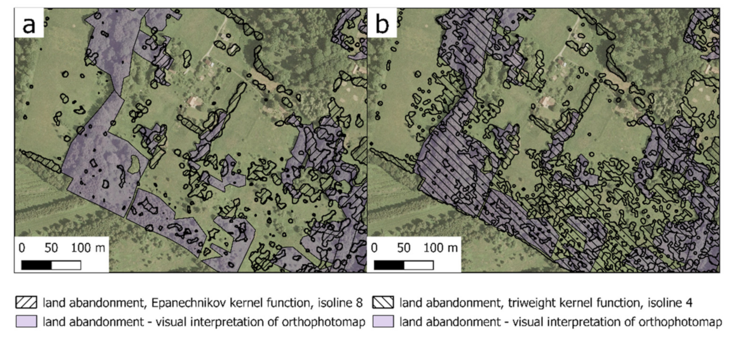
| 1 | Epanechnikov | 8 | 97.4098 | 56.7156 | 107.4600 | 53 |
| 2 | triweight | 4 | 141.8990 | 88.2909 | 82 | |
| 3 | Epanechnikov | 8 | 90.6594 | 53.7292 | 50 | |
| 4 | triweight | 2 | 143.4820 | 79.0786 | 74 | |
| 5 | Epanechnikov | 8 | 78.5410 | 47.9691 | 45 | |
| 6 | triweight | 6 | 82.3856 | 49.4226 | 46 |
Publisher’s Note: MDPI stays neutral with regard to jurisdictional claims in published maps and institutional affiliations. |
© 2021 by the authors. Licensee MDPI, Basel, Switzerland. This article is an open access article distributed under the terms and conditions of the Creative Commons Attribution (CC BY) license (http://creativecommons.org/licenses/by/4.0/).
Share and Cite
Czesak, B.; Różycka-Czas, R.; Salata, T.; Dixon-Gough, R.; Hernik, J. Determining the Intangible: Detecting Land Abandonment at Local Scale. Remote Sens. 2021, 13, 1166. https://doi.org/10.3390/rs13061166
Czesak B, Różycka-Czas R, Salata T, Dixon-Gough R, Hernik J. Determining the Intangible: Detecting Land Abandonment at Local Scale. Remote Sensing. 2021; 13(6):1166. https://doi.org/10.3390/rs13061166
Chicago/Turabian StyleCzesak, Barbara, Renata Różycka-Czas, Tomasz Salata, Robert Dixon-Gough, and Józef Hernik. 2021. "Determining the Intangible: Detecting Land Abandonment at Local Scale" Remote Sensing 13, no. 6: 1166. https://doi.org/10.3390/rs13061166