Semantic Segmentation of Aerial Imagery via Split-Attention Networks with Disentangled Nonlocal and Edge Supervision

Abstract

In this work, we propose a new deep convolution neural network (DCNN) architecture for semantic segmentation of aerial imagery. Taking advantage of recent research, we use split-attention networks (ResNeSt) as the backbone for high-quality feature expression. Additionally, a disentangled nonlocal (DNL) block is integrated into our pipeline to express the inter-pixel long-distance dependence and highlight the edge pixels simultaneously. Moreover, the depth-wise separable convolution and atrous spatial pyramid pooling (ASPP) modules are combined to extract and fuse multiscale contextual features. Finally, an auxiliary edge detection task is designed to provide edge constraints for semantic segmentation. Evaluation of algorithms is conducted on two benchmarks provided by the International Society for Photogrammetry and Remote Sensing (ISPRS). Extensive experiments demonstrate the effectiveness of each module of our architecture. Precision evaluation based on the Potsdam benchmark shows that the proposed DCNN achieves competitive performance over the state-of-the-art methods.

1. Introduction

Land use and land cover (LULC) represents a synthesis of surface elements covered by natural and artificial structures. Land cover data are fundamental to regional planning, ecosystem assessment, environmental modeling and many other studies. Urbanization, globalization and sometimes even disasters lead to rapid changes in the type of LULC [1]. In urban applications, the demand for high-precision and time-efficient LULC mapping products is increasing [2].

With the development of remote sensing technology, new types of aerial sensors, such as unmanned aircraft, can provide time-efficient aerial images with ultra-high ground resolution [3]. Therefore, aerial image interpretation has become an important task in the field of remote sensing. Since the ground resolution of aerial images is better than 10 cm, more details of targets are captured, which brings challenges to the semantic segmentation task. First, heterogeneous manmade objects, such as roads and houses, have high intraclass variance and low interclass variance of the aerial imagery. Second, artificial structures with height drop will generate umbra and falling shadows, thus affecting the spectral characteristics of the pixels.

In recent years, DCNN has performed well in multiple computer vision tasks, such as semantic segmentation, instance segmentation and object detection [4]. Remote sensing image analysis based on DCNN also has aroused widespread research interest and become the current start-of-art method. Deep learning uses an end-to-end approach to obtain the parameterized representation of features and classifiers jointly; it outputs the class likelihoods of each pixel in the image at a time. The key factor for the success of deep learning is that DCNN can extract multiscale contextual information. However, when dealing with pixel-wise semantic segmentation, there is a tradeoff between a larger receptive field and precise pixel positioning [5]. Due to the large size of remote sensing images and the inclusion of more targets, the proportion of edge pixels is higher, and thus the problem of edge blur is more prominent.

Focusing on this problem, the strategy of considering edge detection in the semantic segmentation process has achieved an effective accuracy improvement. At present, the research mainly comes from three aspects as follows: the first is to independently design the edge detection and semantic segmentation network and use the result of the edge detection as the input channel of the semantic segmentation network [5]; a more scalable way is to infer the edge pixel based on the semantic segmentation results, thereby constructing a loss combination of the weighted segmentation loss and the weighted edge detection loss [6]; the third idea comes from the holistically nested edge detection net (HED) [7], the edge detection network and the semantic segmentation network share the same feature extractor, but calculate the results independently, and their losses are combined to train the parameters jointly [8].

In 2015, the residual network structure (ResNet) was proposed, which solved the problem of vanishing gradient in neural networks and made it possible to train deeper and stronger neural networks [9]. In the last few years, especially after 2017, the application of attention mechanism has become another popular stagey for improving the precision of semantic segmentation networks. An attention mechanism is a resource allocation scheme that allocates computing resources to more important tasks [10]. A simple understanding is to increase the weight of the “concerned features/pixels” in hidden layers of the neural network. Since 2015, the attention mechanism has been introduced into the field of image segmentation and expanded from the spatial domain [11,12,13] and channel domain [14,15] to the hybrid domain [16,17,18]. Researchers have explored a variety of methods for combining attention mechanisms in DCNN, and some of them have achieved the highest precision on public benchmarks or and even have a worldwide reputation.

In this paper, we introduce a novel DCNN for semantic segmentation of aerial imagery. The network is based on the encoder–decoder structure and combines inspirations from the latest achievements in the field of computer vision as well as remote sensing image analysis. The proposed pipeline utilizes split-attention networks for feature extraction, which combines the idea of grouped channel attention. To capture the long-range spatial dependencies between pixels and highlight class boundaries, we integrate the disentangled nonlocal (DNL) spatial attention in our network. A depth-wise separable ASPP module is introduced to capture multiscale contextual information meanwhile balance the model performance and computational consumption. Finally, since pixel-wise semantic segmentation requires accurate edge positioning, we design an auxiliary edge detection task to provide edge constraints for semantic segmentation. It shares the same backbone with the semantic segmentation task. The edge loss and segmentation loss are weighted and added as the total loss to train the network parameters jointly. In summary, the main contributions of this study are as follows:

(1)

We propose a novel encoder–decoder network for semantic segmentation of aerial imagery. In the encoder part, we apply the split-attention backbone and combine a depth-wise separable ASPP module for multiscale feature expression. In the decoder part, we use a disentangled nonlocal block to further incorporate spatial attention in our pipeline. We aim to improve the performance of the network through a spatial-channel hybrid attention mechanism;

(2)

We tested the effectiveness of the DNL block in detail from both quantitative evaluation and visualization clues and analyzed the accuracy improvement brought by the DNL block at different positions of the baseline;

(3)

For accurate edge positioning, our pipeline applies a multitask network design. An auxiliary edge detection task is designed to provide edge constraints for semantic segmentation tasks, the two tasks share a common backbone, and the edge loss and segmentation loss are weighted and added as a total loss to train the network parameters jointly.

The remainder of the paper is organized as follows: Section 2 briefly reviews the related works. The architecture of the proposed DCNN is presented in Section 3. Experimental data, training details, analysis of the DNL block and an architecture ablation study are presented in Section 4. Precision evaluation of the proposed DCNN and a comparison with the state-of-the-art methods are discussed in Section 5. Finally, the conclusions of this study are presented in Section 6.

2. Related Works

2.1. Review of DCNN-Based Semantic Segmentation Methods in the Field of Computer Vision

Semantic segmentation is an essential component in visual scene understanding, and DCNN methods have achieved state-of-the-art performance on this task at present. A full convolution network (FCN) is introduced as a milestone of semantic segmentation [19]. In this work, fully connected layers are replaced by convolution layers to build end-to-end neural networks and obtain dense predictions. FCN uses skip connections and upsamplings between shallow and deep layers to generate segmentation results at a 1:8 resolution. To recover the size of feature maps, efforts have been made on convolutional auto-decoders. DeconvNet [20], SegNet [21], and U-net [22] all use a symmetrical encoder–decoder architecture. DeconvNet proposed a deconvolution (transposed convolution) structure. Multiple deconvolutions and upsamplings are combined to gradually recover the spatial resolution of feature maps [20]. The novelty of SegNet is the recorded upsampling; during the max-pooling operation, indexes of the largest pixels in the feature maps are recorded, and the maximum value is assigned to the same position in the corresponding upsampling operation [21]. U-net and its variants are widely applied in medical image analysis. These structures build skip connections between feature maps in encoder and decoder modules to better refine small targets and detailed information [22]

Considering the additional computational expenses of the deconvolution, Chen et al. proposed the DeepLab series of architectures and promoted the application of atrous/dilated convolution [23,24,25,26]. The atrous/dilated convolution is able to extract contextual information of different scales by adjusting a rate parameter. Inspired by the spatial pyramid pooling, DeepLab V2 samples input features with different rates to capture multiscale image context, which is called atrous spatial pyramid pooling (ASPP) [23]. DeepLab V3 further optimizes the structure of the ASPP by applying batch normalization after the atrous convolution and joining two branches of 1$\times$1 convolution and global average pooling [24]. DeepLab V3+ reuses the structure of encoder–decoder, adopts the Xception as the backbone and uses a depth-wise separable convolution to balance time consumption [25].

The application of attention mechanism has become a popular strategy for improving the performance of semantic segmentation networks in recent years. Nonlocal neural networks [11] is an important work among attention research; it focuses on capturing long-range spatial dependencies between pixels. Since the block maintains the size of input feature maps, it can be directly embedded into any existing network. Squeeze and excitation networks (SE) [15] focuses on the dependences across channels. The block learns the weights of channels through a global average pooling layer followed by two fully connected layers, thus selectively excites more related channels and suppresses fewer effective channels. Nonlocal block enhances the expression by gathering specific global information for each pixel; however, a study found that for different query points, the attention maps modeled by the nonlocal block are almost the same. Therefore, the nonlocal block was simplified to query independent and combined with the SE block in this study, thus creating the global context networks (GC) [18]. A more in-depth study of nonlocal block clarified the reason for query independent of the nonlocal block in some image recognition tasks from both formula analysis and visualization. It splits the attention calculation of nonlocal block into a whitened pairwise term and a unary term; each accounts for the relationship between two pixels and the influence of one pixel generally over all pixels [13]. Furthermore, this study proves that the disentanglement of nonlocal is beneficial to the training of both terms. Criss-cross attention network (CCNet) [12] proposed a twice-recurrent spatial attention block. In each circle, only the relationship between the current pixel and pixels in the same row or column as the current pixel are considered. This reduces the memory occupation and computational complexity of the module. The latest research on combining attention mechanism in semantic segmentation also includes convolutional block attention module (CBAM) [15] and dual attention network (DANet) [14], both of them introduce attention blocks in spatial and channel dimensions simultaneously.

2.2. Review of DCNN-Based Semantic Segmentation Methods in the Field of Remote Sensing

Semantic segmentation plays an important role in the field of remote sensing. Relying on the development of deep learning, various excellent solutions based on the DCNN have been presented recently. The ResUNet-a introduces a novel, fully convolutional network for semantic segmentation [6]. The architecture is based on the U-Net backbone, and various classic modules, including residual connections, atrous convolutions, pyramid scene parsing pooling, and multitasking inference, are incorporated to improve the performance of the network. In addition, a variant of the dice loss function is introduced to speeds up the convergence of training and improves the overall accuracy. Liu et al. [27] proposed a self-cascaded convolutional neural network (ScasNet) for semantic segmentation on VHR images. The encoder is departed from the VGG-Net [28], and multiscale contextual features are aggregated hierarchically from coarse to fine. Feature resolution was gradually recovered using a decoder structure that is symmetrical to the encoder structure. In addition, residual modules are applied in multiple branches of the network to further correct the latent fitting residual caused by semantic gaps in multifeature fusion. Panboonyuen et al. [29] presented a convolutional network, which is consists of a high-resolution representation (HRNet) [30] backbone, a set of feature fusion blocks, channel attention blocks and deconvolution blocks. In feature fusion, multilayer features of the HRNet are combined with features obtained by the global convolutional network (GCN) [31] to enhance local-global expression. In the decoder module, feature maps of different resolutions are further fused through a depth-wise separable convolution. Liu et al. [32] proposed an hourglass-shaped network (HSN) for semantic segmentation of high-resolution aerial imagery. Its encoder part and decoder part both partially use the inception modules, and two jump-connected residual structures are linked between the features in the encoder and decoder modules.

According to our best knowledge, the first study to introduce edge constraints in DCNN for semantic segmentation of remote sensing images is [5]. In this work, HED [7] is combined with SegNet, FCN, and UNet, respectively. The two tasks of edge detection and semantic segmentation were connected in an end-to-end convolutional neural network successively. The color image and digital surface model (DSM) data are input into the HED network as two parallel branches first to obtain the edge probability map, and then the maps are concatenated with the raw data and input into the semantic segmentation networks. Liu et al. [8] proposed a novel edge loss reinforced semantic segmentation network (ERN) to reduce the semantic ambiguity through spatial boundary context. In both encoder and decoder modules of the architecture, edge pixels are predicted by two middle-layer features, and the final loss is composed of two weighted detection losses and a weighted segmentation loss. The ERN simultaneously achieves semantic segmentation and edge detection results without significantly increasing the model complexity.

In conclusion, the exploration of DCNN in semantic segmentation is moving towards deeper networks, less computational complexity, and better retention of detailed information. Popular backbone include VGGnet [28], ResNet [9], ResNeSt [33], HRNet [34] and their variants. Popular strategies to enhance the performance of backbones include attention mechanism, local-global feature fusion, edge supervision, data augmentation, etc. Some comprehensive reviews of DCNN based semantic segmentation methods are [35,36,37,38].

3. Method

In this section, we introduce the architecture of the proposed semantic segmentation network in full detail. Section 3.1 introduces our overall network structure, and Section 3.2 describes the ResNeSt backbone. The depth-wise separable ASPP module is delineated in Section 3.3. The disentangled nonlocal attention block is shown in Section 3.4. Finally, the content about edge detection used in this article is introduced in Section 3.5.

3.1. Architecture

Our pipeline (Figure 1) combines the following set of modules:

• A split-attention network is used as the backbone for feature extraction. It inherits the structural characteristics of ResNet; specifically, it replaces the residual blocks with split-attention blocks, which combines the idea of grouped channel attention;
• Depth-wise separable ASPP module is used to capture multiscale contextual information. This inspiration comes from the DeepLab series. The ASPP module uses multiple parallel/cascade atrous convolutions with different rates to capture multiscale contextual information while maintaining the spatial resolution of the feature map. The depth-wise separable ASPP is a combination of the standard ASPP and depth-separable convolution, which has been proven to be able to effectively reduce the number of parameters while maintaining (or slightly improving) the module’s performance;
• A disentangled nonlocal attention module is used to calculate spatial attention weights. It can obtain the long-distance dependency between every two pixels and also pays attention to the edge pixels in the image. Channel attention was considered in the backbone of ResNeSt, and we further design the integration of a spatial attention module in our network to obtain more expressive features;
• In the task of semantic segmentation of remote sensing images, an important challenge is the determination of details and edges, which is the drawback of continuous pooling to obtain large receptive fields. In order to obtain a more accurate edge and location information, our pipeline incorporates an edge detection task. During model training, we combine it with the segmentation task to build a comprehensive loss function.

3.2. Backbone

We choose the split-attention networks (ResNeSt) [33] as the backbone in our work for feature extraction for the following two reasons: (1) good training and inference speed and less memory cost; (2) compared with variants of ResNet with a similar amount of parameters, ResNeSt have achieved state-of-art accuracy on the ADE20K and Cityscapes datasets. In downstream tasks, such as object detection and semantic segmentation, the authors obtained more than 3% accuracy improvement by only replacing the original ResNet backbone.

ResNeSt inherits the structural characteristics of ResNet; specifically, it replaces the residual blocks with split-attention blocks. A comparison of the structure of ResNeSt and ResNet is shown in Table 1. More details of the split-attention networks are described in the following two subsections.

3.2.1. Split-Attention Block

The split-attention block (SA) is a computational unit; it contains three parts of 1$\times$1 convolution, split-attention module and 1$\times$1 convolution in sequence. The split-attention module includes two parts: feature map group and split-attention within each group. Input features are first divided into $K$ groups according to a $cardinality$ hyperparameter, and each group is further divided into $R$ mini groups according to an $radix$ hyperparameter. Features within each cardinal group participate in independent channel-wise attention; correlation of features between different cardinal groups are not considered. In the original work of ResNeSt, the authors comprehensively consider the scalability, speed, module accuracy and memory consumption of the block and recommended the parameter combination of $K=1$ and $R=2$. We follow the author’s suggestions and set a similar value of parameters to complete our work in this paper. In the following introduction, we pay attention to the structure of the SA module when $K=1$ and $R=2$.

As shown in Figure 2, in a SA module ($K=1$, $R=2$), input features are first split through a group convolution with $group=2$,$stride=1$, and a kernel size of 3$\times$3, followed by which, two branches $U_1$ and $U_2$ are obtained through batch normalization and ReLU activation. Note that each branch has the same number of channels as the input features. Therefore, a representation of the cardinal group can be acquired by fusion via an element-wise summation across the two splits:

$$U_c=U_1+U_2.$$

(1)

Based on the fused features, a vector $V\in {\mathbb{R}}^c$ is calculated through the global average pooling operation; therefore, each element in the vector is considered to have embedded channel-wise global information. Specifically, the c-th element of $V$ is calculated as:

$$V_c={\mathcal{F}}_{gp}\left(U_c\right)=\frac{1}{H \times W}\sum _{i=1}^H\sum _{j=1}^W{U}_c\left(i,j\right)$$

(2)

Subsequently, a vector $\mathcal{G}\in {\mathbb{R}}^{2c}$ is calculated through a channel-wise attention block applied by two consequent fully connected layers. The number of nodes in the first fully connected layer is $c/s$ ($s$ represents the reduction ratio), and the number of nodes in the second fully connected layer is $c\cdot r$, where $r$ equals the radix hyperparameter $R$. Furthermore, the vector $\mathcal{G}$ is divided into two vectors of equal length: ${\mathcal{G}}_1$ and ${\mathcal{G}}_2$. And an r-softmax operation is performed to obtain the normalized attention weight of each channel. Please note that the effect of r-softmax is to make the sum of the c-th element of ${\mathcal{G}}_1$ and the c-th element of ${\mathcal{G}}_2$ equals to 1. Each feature in the cardinal group is recalculated through element-wise product, and furthermore, element-wise add is used to fuse the two branches and obtain the final feature maps $\tilde{U}$:

$$\tilde{U}={\mathcal{G}}_{1c}\cdot U_{1c}+{\mathcal{G}}_{2c}\cdot U_{2c} , {\mathcal{G}}_{1c}+{\mathcal{G}}_{2c}=1$$

(3)

3.2.2. Split-Attention Networks

Similar to the ResNet structure, ResNeSt is composed of multiple stacked SA blocks as bottlenecks. The hyperparameters ($cardinality$, $radix$, and $reduction ratio$) set in the SA block in our experiments are $\left\{1, 2, 2\right\},$ respectively. The net structure of the 50-layer ResNeSt is shown in Table 1; the number of bottlenecks stacked in each stage is $\{3, 4, 6, 3\}$.

Table 1. Network structure of ResNet-50 and ResNeSt-50. The second column refers to the ResNet-50, and the third column refers to the ResNeSt-50. The input stem of split-attention networks (ResNeSt)-50 uses three consecutive 3 $\times$ 3 convolutions to replace a 7$\times$7 convolution. The residual/split-attention blocks are in square brackets; the number of blocks stacked in each stage is displayed outside the brackets.

Module	ResNet-50	ResNeSt-50
Input stem	$7\times 7, 64, \mathrm{stride} 2$	$\begin{array}{c}3\times 3, 64, \mathrm{stride} 2\\ 3\times 3, 64, \mathrm{stride} 1\\ 3\times 3, 128, \mathrm{stride} \end{array}$
	$3\times 3,max pool, \mathrm{stride} 2$	$3\times 3,max pool, \mathrm{stride} 2$
Stage 1	$\left[\begin{array}{l} 1\times 1, 64\\ 3\times 3, 64\\ 1\times 1, 256\end{array}\right]\times 3$	$\left[\begin{array}{l}1\times 1, 128\\ SA\left[K=1,R=2,s=2,r=1\right], 128\\ 1\times 1, 256\end{array}\right]\times 3$
Stage 2	$\left[\begin{array}{l} 1\times 1, 128 \\ 3\times 3, 128\\ 1\times 1, 512\end{array}\right]\times 4$	$\left[\begin{array}{l}1\times 1, 256\\ SA\left[K=1,R=2,s=2,r=1\right], 256\\ 1\times 1, 512\end{array}\right]\times 4$
Stage 3	$\left[\begin{array}{l}1\times 1, 256\\ 3\times 3, 256\\ 1\times 1, 1024\end{array}\right]\times 6$	$\left[\begin{array}{l}1\times 1, 512\\ SA\left[K=1,R=2,s=2,r=2\right], 512\\ 1\times 1, 1024\end{array}\right]\times 6$
Stage 4	$\left[\begin{array}{l}1\times 1, 512\\ 3\times 3, 512\\ 1\times 1, 2048\end{array}\right]\times 3$	$\left[\begin{array}{l}1\times 1, 1024\\ SA\left[K=1,R=2,s=2,r=4\right], 1024\\ 1\times 1, 2048\end{array}\right]\times 3$

Table 1. Network structure of ResNet-50 and ResNeSt-50. The second column refers to the ResNet-50, and the third column refers to the ResNeSt-50. The input stem of split-attention networks (ResNeSt)-50 uses three consecutive 3 $\times$ 3 convolutions to replace a 7$\times$7 convolution. The residual/split-attention blocks are in square brackets; the number of blocks stacked in each stage is displayed outside the brackets.

Module	ResNet-50	ResNeSt-50
Input stem	$7\times 7, 64, \mathrm{stride} 2$	$\begin{array}{c}3\times 3, 64, \mathrm{stride} 2\\ 3\times 3, 64, \mathrm{stride} 1\\ 3\times 3, 128, \mathrm{stride} \end{array}$
	$3\times 3,max pool, \mathrm{stride} 2$	$3\times 3,max pool, \mathrm{stride} 2$
Stage 1	$\left[\begin{array}{l} 1\times 1, 64\\ 3\times 3, 64\\ 1\times 1, 256\end{array}\right]\times 3$	$\left[\begin{array}{l}1\times 1, 128\\ SA\left[K=1,R=2,s=2,r=1\right], 128\\ 1\times 1, 256\end{array}\right]\times 3$
Stage 2	$\left[\begin{array}{l} 1\times 1, 128 \\ 3\times 3, 128\\ 1\times 1, 512\end{array}\right]\times 4$	$\left[\begin{array}{l}1\times 1, 256\\ SA\left[K=1,R=2,s=2,r=1\right], 256\\ 1\times 1, 512\end{array}\right]\times 4$
Stage 3	$\left[\begin{array}{l}1\times 1, 256\\ 3\times 3, 256\\ 1\times 1, 1024\end{array}\right]\times 6$	$\left[\begin{array}{l}1\times 1, 512\\ SA\left[K=1,R=2,s=2,r=2\right], 512\\ 1\times 1, 1024\end{array}\right]\times 6$
Stage 4	$\left[\begin{array}{l}1\times 1, 512\\ 3\times 3, 512\\ 1\times 1, 2048\end{array}\right]\times 3$	$\left[\begin{array}{l}1\times 1, 1024\\ SA\left[K=1,R=2,s=2,r=4\right], 1024\\ 1\times 1, 2048\end{array}\right]\times 3$

We adopt the ResNet-D structure in the ResNeSt, which is different from the standard ResNet structure in two points: (1) the 7 $\times$ 7 convolution in the input stem is replaced with three consecutive 3 $\times$ 3 convolutions; (2) the downsampling in the identity branch adds a 2 $\times$ 2 pooling operation before the original 1 $\times$ 1 convolution. In addition, in order to maintain the spatial resolution of the feature map not less than 1/8 of the original image, we apply the atrous convolutions, and the rates in four stages are set to $\left\{1, 1, 2, 4\right\},$ respectively.

By changing the number of bottlenecks in each stage, networks with different layers can be obtained. In this article, we also used the 101-layer ResNeSt as the backbone in some experiments, and the number of bottlenecks in each stage is set to $\left\{3, 4, 23, 3\right\},$ respectively.

As the depth of the network increases, the features of the convolutional layer have a larger receptive field. The shallow convolutions learn more basic image descriptors, while the deep feature maps pay more attention to the semantic structure. In order to visually show the difference between shallow and deep features, we display few examples of feature maps output by each stage of the ResNeSt-50 in Figure 3. Shallow features learn more local details from the image, such as points and lines, while deep features are more abstract and difficult to understand. Even so, one can still recognize that specific classes are emphasized. These provide the basis for the design of our edge detection module and decoder module.

3.3. Depth-Wise Separable ASPP Module

An atrous convolution with $rate=r$ inserts $r-1$ zeros between adjacent elements of the original convolution kernel, thereby expanding the original receptive field from $k\times k$ to $k + \left(k-1\right)\left(r-1\right)$ without introducing additional parameters. To express the contextual information of a center pixel, the ASPP module superimposes information of multiple scales by atrous convolution with different rates in parallel [23].

The atrous separable convolution is a combination of the atrous convolution and the depthwise separable convolution. A schematic diagram of the depth-wise separable convolution is shown in Figure 4. The depth-wise separable ASPP module uses atrous separable convolutions instead of atrous convolutions to capture multiscale contextual information. It has been proven that a utilize of the atrous separable convolutions in the ASPP will not cause a reduction in model accuracy but can effectively reduce computational consumption [25].

The architecture of the depth-wise separable ASPP module used in our module is shown in Figure 5. Our depth-wise separable ASPP module contains 5 branches in parallel, namely (a) a 1$\times$1 convolution, (b) three 3$\times$3 atrous separable convolutions, and (c) a global average pooling layer. Specifically, we input the feature maps output by the 4th stage of the ResNeSt-50 into the depth-wise separable ASPP module. It has 2048 input channels, and the number of output channels of each branch is 512. These features are then concatenated and passed through a 1$\times$1 convolution with 512 kernels for feature fusion and dimension reduction.

Based on our experimental data, rates are rigorously set in the depth-wise separable ASPP module. Limited by hardware conditions, the frame size of our input image is 300$\times$300. Therefore, the size of the corresponding feature maps output by stage 4 is 38 $\times$ 38. According to the calculation formula of receptive field based on the atrous convolution, we adopt new rates setting of $\left(6,12,18\right),$ which corresponds to a maximum distance on the feature map of $\left(13, 25, 37\right)$ and a maximum distance on the original image of $\left(104, 200, 296\right)$.

3.4. Disentangled Nonlocal Block

Grouped channel attention was introduced in the ResNeSt backbone, and we further design the integration of the spatial attention module in our network to enhance its spatial expression. The uniqueness of disentangled nonlocal (DNL) is that it can simultaneously express the long-distance dependence between pixels and highlight the class edges in the image, which is just important for remote sensing image interpretation.

A brief introduction of the derivation process of the DNL module is shown below; for more rigorous reasoning details, please refer to the original source of the DNL block [13]. The DNL module is explained as a disentangled nonlocal block, and an expression of the original nonlocal block is:

$${\mathit{y}}_i=\sum _{j\in \mathsf{\Omega }}\omega \left({\mathit{x}}_i,{\mathit{x}}_j\right)g\left({\mathit{x}}_j\right),$$

(4)

in this expression, $\mathsf{\Omega }$ represents all positions of the feature map, ${\mathit{x}}_i$ represents the input feature at pixel $i$, ${\mathit{y}}_i$ is the corresponding output feature, and ${\mathit{x}}_j$ represents any pixel on the feature map. The $\omega \left({\mathit{x}}_i,{\mathit{x}}_j\right)$ is a pairwise function, which is used to calculate the similarity between pixel $i$ and pixel $j$, $g\left(·\right)$ is an input transformation function. In particular, the similarity in an embedding space can be calculated by an extension of the Gaussian function:

$$\omega \left({\mathit{x}}_i,{\mathit{x}}_j\right)=\sigma \left({\mathit{q}}_i^T{\mathit{k}}_j\right)=\frac{\exp \left({\mathit{q}}_i^T{\mathit{k}}_j\right)}{{\sum }_{t\in \mathsf{\Omega }} \exp \left({\mathit{q}}_i^T{\mathit{k}}_t\right)}$$

(5)

in this formula, ${\mathit{q}}_i=W_q{\mathit{x}}_i$, ${\mathit{k}}_j=W_k{\mathit{x}}_j$, and $\sigma \left(·\right)$ represents a softmax operation. Furthermore, a $whitened dot product$ ${\left({\mathit{q}}_i-{\mathit{\mu }}_q\right)}^T\left({\mathit{k}}_j-{\mathit{\mu }}_k\right)$ between ${\mathit{q}}_i$ and ${\mathit{k}}_j$ is introduced, and we obtained the following formula:

$${\mathit{q}}_i^T{\mathit{k}}_j={\left({\mathit{q}}_i-{\mathit{\mu }}_q\right)}^T\left({\mathit{k}}_j-{\mathit{\mu }}_k\right)+{\mathit{\mu }}_q^T{\mathit{k}}_j+{\mathit{q}}_i^T{\mathit{\mu }}_k+{\mathit{\mu }}_q^T{\mathit{\mu }}_k,$$

(6)

where ${\mu }_q=\frac{1}{|\Omega |}{\sum }_{i\in \Omega } {\mathit{q}}_i$ , and ${\mathit{\mu }}_k=\frac{1}{\left|\mathsf{\Omega }\right|}{\sum }_{j\in \mathsf{\Omega }} {\mathit{k}}_j$ represent the average value of $\mathit{q}$ and $\mathit{k}$ respectively. Since the last two terms are factors that appear in both the numerator and denominator of equation 5, they are eliminated. And the disentangled expression of nonlocal is finally obtained:

$$\omega \left({\mathit{x}}_i,{\mathit{x}}_j\right)=\sigma \left({\mathit{q}}_i^T{\mathit{k}}_j\right)=\sigma \left(\underset{pairwise}{\underbrace{{\left({\mathit{q}}_i-{\mathit{\mu }}_q\right)}^T\left({\mathit{k}}_j-{\mathit{\mu }}_k\right)}}+\underset{unary}{\underbrace{{\mathit{\mu }}_q^T{\mathit{k}}_j}}\right).$$

(7)

Through the above transformations, attention in nonlocal is decomposed into a whitened pairwise term and a unary term. The whitened pairwise term learns the feature relationship between pixels, and the unary term learns salient edges. The two factors are mutual factors in the gradient derivation of backpropagation. When any one of them is as small as close to zero, the gradient value will be extremely small, and the training of both terms will be hindered. Thus, a disentanglement of nonlocal is beneficial to the training of both terms [13]. A more detailed analysis of the effect of the DNL module in our architecture is shown in Section 4.4 through quantitative evaluation and visualization analysis.

3.5. Edge Detection

In order to better determine the edge between classes, we combine the edge detection task in our network. Specifically, as shown in the yellow dashed box in Figure 1, we combine the feature maps output by stage 1, stage 2, and the depth-wise separable ASPP in the encoder structure to detect edges. Output features of stage 2 and the depth-wise separable ASPP are adjusted to the same size as the output of stage 1 through upsampling, and then these feature maps are concatenated and passed through a 1 $\times$ 1 convolution for feature fusion. Finally, a 1 $\times$ 1 convolution is applied to obtain the edge probabilities of each pixel. As an aid to the semantic segmentation task, we use a relatively simple method to complete the edge extraction task, avoiding the introduction of too many new parameters and calculations.

We choose the combination of low-layer, middle-layer, and output features of the depth-wise separable ASPP module because deep-layer features express more high-level semantic structure and extract less basic image elements. Relatively, the low-layer feature maps can better retain basic image descriptors, and the multiscale fusion result of the depth-wise separable ASPP helps maintain the integrity of segmentation targets.

Considering the imbalance of the number of edge pixels and non-edge pixels in the image, we draw inspiration from the boundary loss [39] and use the following function as the loss function for edge detection:

$$los{s}_{eg}=1-F_1$$

(8)

where $F_1=2\times \left(precision\times recall\right)/\left(precision+recall\right)$ represents a comprehensive evaluation of recall and precision. In order to better explain the principle and differentiability of the edge detection loss function used in this work, we provide detailed pseudocodes and corresponding example diagrams in Appendix A for calculating the $los{s}_{eg}$.

The loss function for semantic segmentation in the proposed network is the standard cross-entropy:

$$los{s}_{seg}=-\frac{1}{N}\sum _{i=1}^{K}I⟦y_i=j⟧\log (y_i=j|x_i|),$$

(9)

where $y_i$ is the ground truth class of pixel $i$, $N$ is the number of pixels in a batch, K is the number of classes,$p$ represents the probability that the pixel $i$ belongs to the j-th class and $I⟦y_i=j⟧$ is an indicator function; it takes 1 only when $y_i=j$, and 0 in other cases.

The global loss function in training is calculated by the summation of weighted semantic segmentation loss and weighted edge detection loss:

$$los{s}_{total}= \alpha ·los{s}_{eg}+\beta ·los{s}_{seg}$$

(10)

The selection of hyperparameters $\alpha$ and $\beta$ will affect the convergence and accuracy of the DCNN model. Ideally, these parameters can be adjusted dynamically, and further research is necessary. However, considering the complexity of the experiment, we tested three different sets of parameter combinations of $\alpha$ and $\beta$, each is {0.15, 1}, {0.5, 1} and {1, 1}. All three DCNN models can converge within the maximum number of iterations. In this case, we choose the parameter combination with the highest semantic segmentation accuracy and set $\alpha$ to 0.15, $\beta$ to 1, respectively. Appendix B shows the training evolution of the three models.

4. Experiments

4.1. Datasets

We evaluated the proposed method on two open benchmarks provided by ISPRS for the 2D semantic labeling challenge [40]. Both datasets provide matched orthophotos and the corresponding hand-labeled ground truth.

Potsdam Benchmark [41]: Potsdam is a typical historic city with many large buildings, neat roads, and much traffic. The airborne image dataset consists of true color (R,G,B) orthophotos and corresponding hand-labeled ground truth. Overall, 38 image blocks with a size of 6000 × 6000 are clipped from orthophotos, and the ground sampling distance is 5 cm.

Vaihingen Benchmark [42]: Vaihingen is a small village with many detached multi-story buildings, more vegetation cover and less traffic. The airborne image dataset consists of false color (NIR,R,G) orthophotos and corresponding hand-labeled ground truth. In total, 33 different sizes of blocks are clipped with a ground sampling distance of 9 cm. The size of each patch is about $2000\times 2500$ pixels. Some examples of the original orthophotos and ground truth provided by the two datasets are shown in Figure 6.

Since 2018, ISPRS has provided ground truth for all image patches. However, in order to facilitate algorithm comparison, the training data and test data of our experiments are the same as those set in the competition. Specifically, the Vaihingen benchmark uses 16 patches for training and the remaining 17 patches for method evaluation, while the Potsdam benchmark sets the number of training and test patches to 24 and 14, respectively. Some DCNN-based methods have achieved high semantic segmentation accuracy by using only spectral data. At the same time, considering that DSM is not provided under general circumstances, our experiment utilizes only spectral data to complete the semantic segmentation task.

4.2. Evaluation Metrics

Overall, accuracy (OA) and F1 score are used to evaluate model performance. The F1 score considers correctness and completeness comprehensively, it can be calculated based on the following formulas:

$$F_1=2\times \frac{ \mathrm{precision} \times \mathrm{recall} }{ \mathrm{precision} + \mathrm{recall}}$$

(11)

where

$$\mathrm{precision} =\frac{TP}{TP+FP}, \mathrm{recall} =\frac{TP}{TP+FN}$$

(12)

the $TP$, $FP$, and $FN$ stand for true positive, false-positive, and false-negative, respectively. These indexes are calculated through confusion matrices, in which $TP$ are the main diagonal elements, $FP$ is the sum of per column excluding the main diagonal elements, and $FN$ is the sum of per row excluding the main diagonal elements. The OA is calculated using the trace of the matrix divided by the pixel number of the image.

4.3. Training Details

The training set was preprocessed by a series of data augmentation transformations. The initial size of the input aerial images is 600 × 600; convert them to a random size (ratio 0.5–2), and then randomly crop them to 300 × 300. Randomly flip the images along the vertical direction with a probability of 0.5 and add a photometric distortion. Finally, images were normalized by subtracting the mean value of each channel.

In our experiment, all neural networks are trained using stochastic gradient descent (SGD) [43] with a momentum of 0.9 and a weight decay of 0.0005. Poly-learning rate policy is employed; that is, the learning rate is calculated by the product of the base learning rate and ${\left(1-\mathrm{iter}/\mathrm{iter}\_\max \right)}^{power}$. In all our experiments, the base learning rate is set to 0.01 and the power is set to 0.9. The maximum number of iterations for our training is, and all comparison experiments are consistent.

In the training phase, an auxiliary loss for semantic segmentation is added on the output of stage 4 with a weight of 0.4, and the auxiliary loss is not used for inference in the testing phase. In general, the auxiliary head is conducive to network convergence and can help avoid model overfitting. We initialize part of the network from a pretrained 50-layer ResNeSt model on the Cityscape dataset. Then we fine-tune the model on our experimental datasets.

Our experiments are conducted on an Ubuntu 16.04 platform equipped with an Nvidia GeForce 1080Ti. Due to hardware limitations, our batch size is set to 2. It takes about 12 h to complete the training of a standard ResNeSt-50.

4.4. DNL Block Experimental Analysis

The network implementation of the DNL block is briefly shown in Figure 7. For the whitened pairwise term, the key and query are first calculated by a 1$\times$1 convolution separately, and they are each whitened by subtracting the mean value. Subsequently, the key and query tensors are reshaped and multiplied, and then the attention matrix ($\mathrm{HW}\times \mathrm{HW}$) is obtained through softmax. For unary term, the attention matrix is directly calculated through 1$\times$1 convolution and softmax operations, and then the values are further copied and expanded to a size of ($\mathrm{HW}\times \mathrm{HW}$).

We compared semantic segmentation results of our architecture when the DNL block was inserted into different positions in the pipeline. Each time a single DNL block is inserted into different stages of the ResNeSt-50 or the last layer before semantic segmentation. We use only one DNL block in our architecture in consideration of its large memory cost. In order to preserve the resolution of the feature map, we apply atrous convolution in the ResNeSt, and the feature maps of the 1st, 2nd, 3rd, and 4th stage are {$\frac{1}{4}, \frac{1}{8},\frac{1}{8}, \frac{1}{8}$} of the input image, respectively. To express feature similarity between any two pixels in the image, the DNL block contains a large matrix (${38}^2\times {38}^2$) calculation, and brings a huge amount of parameters. In our experiment, the parameters of the correlation matrix are about 800 Mb ($\mathrm{whitened} \mathrm{pairwise}\approx 500 \mathrm{Mb}, \mathrm{and} \mathrm{unary}\approx 300 \mathrm{Mb}$).

In this set of experiments, we adopt the ResNeSt-50 as the backbone, utilized the depth-wise separable ASPP block to extract and fuse multiscale features, and employed the encoder–decoder architecture shown in Figure 1 to maintain and recover the resolution of the feature maps. Please note that in order to avoid introducing interference factors, we did not incorporate the edge detection task in the network during the testing of the DNL block. The same data augmentation and model optimization strategies are applied for all training processes.

Table 2. Precision comparison (OA, %) of networks with embedding a DNL block into different positions of the encoder–decoder architecture.

Model, RS50	Potsdam	Vaihingen
baseline	88.64	87.94
st1	89.87	88.31
st2	89.90	88.52
st3	90.02	88.58
st4	89.82	88.44
last_layer	90.44	88.97

displays the overall accuracy of embedding a DNL block to different positions of the encoder–decoder structure. It was found that inserting the DNL block into each stage of ResNeSt brings an improvement in model accuracy, and the results of stage 2 and stage 3 are slightly better than the results of stage 4 and stage 1. A possible explanation is that stage 1 contains a less semantic message, while stage 4 has too wide a receptive field to provide accurate spatial information. It is worth noting that adding the DNL before the last segmentation layer brings the greatest precision improvement over the baseline. It is presumably because multiscale fusion features have provided rich semantic and location information in the last layer.

In order to show the effect of the DNL block more vividly, samples of attention maps obtained by both terms in the DNL block are displayed in Figure 8. From the middle three columns, it can be observed that in the whitened pairwise term, pixels belonging to a class similar to the query points are assigned higher weights. This is exactly consistent with the physical meaning of the term that represents the similarity between pixels.

The visualization clues of the unary term are clear. As indicated in the last column in Figure 8, the unary term is more sensitive to the edge pixels between targets; the distribution of the weight of these pixels is significantly higher. In addition, we observe that the edges inside objects (such as the edge pixels of the “chimney” on the “building”) are not assigned extremely high unary weights. This may help determine the class extent in semantic segmentation tasks.

4.5. Architecture Ablation Study

We designed a group of ablation experiments to test the effect of each module in our proposed network. Since our goal is to compare the effects of the modules instead of obtaining the most competitive accuracy, we have completed the set of experiments on a baseline of 50-layer ResNeSt for less time cost.

We first trained the basic ResNeSt-50 as the baseline and then tested the segmentation accuracy of the network with the edge detection task added, or the DNL module added, respectively. The effectiveness of the whitened pairwise term and the unary term of the DNL module were further analyzed. Finally, we tested the segmentation accuracy of the proposed architecture, which combines all the ResNeSt-50, edge detection task and DNL modules.

Quantitative analysis: The results of our consequence of experiments on the Potsdam and Vaihingen datasets are shown in

Table 3. Quantitative analysis (%) of the components in the proposed model based on the Potsdam dataset. The average F1 score was calculated using all classes expect the background. All results are based on an edge-erosion statistic.

Methods	Building	Car	Low_veg	Impervious	Tree	OA	Avg_F1
ResNeSt-50	93.69	86.21	87.22	88.89	87.16	89.34	87.33
RS+DNLLAST	94.56	89.52	87.32	91.27	87.32	90.44	89.14
RS+UnaryLAST	94.67	90.52	86.36	89.31	86.92	90.12	88.91
RS+PairwiseLAST	93.97	87.49	87.32	88.98	87.39	89.59	87.63
RS+Edge	94.76	89.12	86.36	90.95	87.27	90.36	89.03
RS+Edge+DNLLAST	94.80	89.46	87.62	91.20	87.45	90.82	89.31

and

Table 4. Quantitative analysis (%) of the components in the proposed model based on the Vaihingen dataset. All results are based on an edge-erosion statistic.

Methods	Building	Car	Low_veg	Impervious	Tree	OA	Avg_F1
ResNeSt-50	93.28	84.09	79.21	91.45	87.62	87.32	87.57
RS+DNLLAST	93.84	85.89	82.84	92.69	88.49	88.14	88.82
RS+UnaryLAST	93.72	85.71	79.93	91.85	87.41	87.91	88.54
RS+PairwiseLAST	93.41	84.83	82.22	91.72	87.77	87.83	88.41
RS+Edge	94.20	85.94	80.28	92.07	87.32	87.75	88.78
RS+Edge+DNLLAST	94.88	85.96	82.97	92.69	88.24	88.84	89.04

. Based on the Potsdam dataset, the overall accuracy of the baseline (ResNeSt-50) reached 89.34%, and the average F1 score was 87.33%. Adding DNL to the last layer of the pipeline increased the model’s OA by 1.1% and F1 score by 1.81%. The combination of edge detection tasks increased the OA of the baseline by 1.02% and the F1 score by 1.7%. Adding the DNL module and the edge detection task to ResNeSt-50 simultaneously obtained the highest overall accuracy of 90.82%, and the improvement of OA and F1 score is 1.48% and 1.98%, respectively. Focusing on the DNL module, both unary and whitened pairwise terms promote the improvement of model accuracy, and the accuracy improvement brought by the unary term exceeds that of the whitened pairwise term.

In terms of details, the addition of the DNL module has improved the segmentation precision of all classes, and the combination of edge detection tasks has a significantly more positive effect on the accuracy of buildings, cars, and impervious classes. One possible reason is that the edges of buildings and cars are sharper and easier to determine. On the contrary, even for a human, the boundaries of low vegetation and trees cannot be distinguished well. Interestingly, this is consistent with the performance of the DNL’s unary term in each class, which tends to highlight edge pixels.

Based on the Vaihingen dataset, the OA of the baseline (ResNeSt-50) reached 87.32%, and the average F1 score reached 87.57%. Adding DNL to the last layer of the pipeline can increase the model’s OA by 0.82% and F1 score by 1.25%. Among them, the unary term is more effective on buildings, cars and low vegetation, while the whitened term has a positive effect on each class and performs best on the low vegetation class. Among all classes, edge detection can relatively more improve the accuracy of buildings, low vegetation and cars, which is similar to the performance of the unary term. Adding both the DNL module and the edge detection task to the ResNeSt-50 obtained the highest overall accuracy of 89.04%, and the improvement of OA and F1 score was 1.52% and 2.47%, respectively.

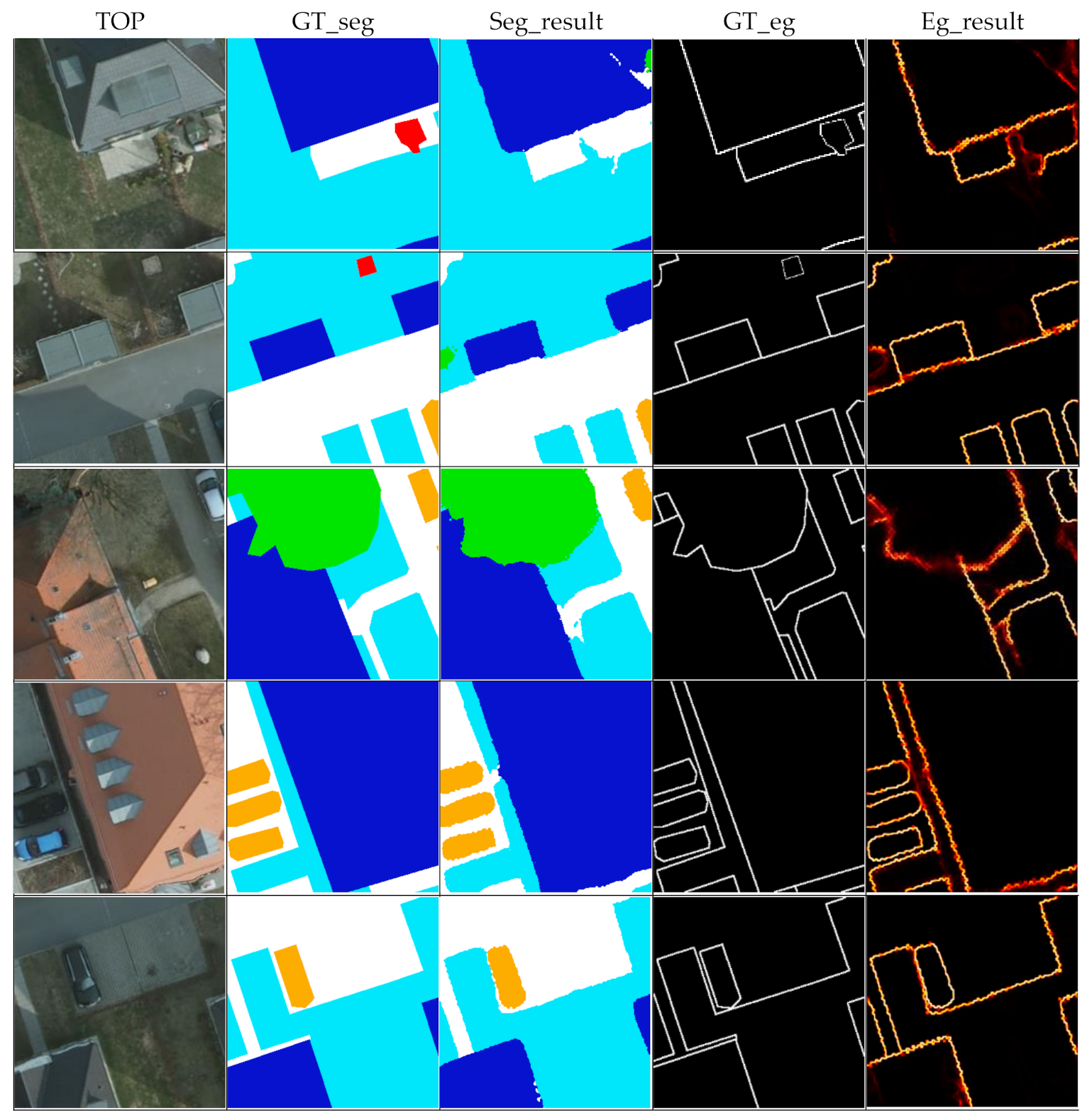
Visualization analysis: we show some of the test results of these two datasets in Figure 9 and Figure 10; from left to right are the original image, ground truth, and model segmentation results. The field of view gradually increases from top to bottom, from details to the whole.

Model information corresponding to each abbreviation is: (1) ResNeSt-50: baseline architecture; (2) RS+Edge: combine edge detection task in the baseline to provide boundary constraints for semantic segmentation; (3) RS+DNL_LAST: insert a DNL module into the last layer before semantic segmentation in the baseline; (4) RS+Edge+DNL_LAST: combine edge detection task and DNL block in the baseline simultaneously.

Based on the Potsdam dataset, almost all models perform well in car detection and can cover cars relatively completely. The main challenge of building detection is the completeness of the segmentation results, especially for buildings with vegetation growing on the roof. Determining the edges between trees and low vegetation is the main difficulty in the semantic segmentation task.

Edge constraints further optimize the contour lines of each class, their edges are much sharper, and the positioning is more accurate, so the structure of targets is more complete. From the perspective of the details of each class, the edge constraint brings the most obvious optimization of the buildings and cars. It detects some missing structures of buildings and cars, and the edges are closer to the ground truth. The edge positioning between low vegetation and trees is also clearer but still insufficient. The application of the DNL attention module enhances the semantic constraints between classes, improves the labeling consistency within targets, and eliminates most salt and pepper noise. Generally, the result of “RS+Edge+DNL_LAST“ has the best visual effect, with the least misclassification in each class and the sharpest target edge.

The visualization effect based on the Vaihingen dataset is basically the same as that of Potsdam. Edge constraints play a positive role in determining the edges of buildings and cars; however, it has no obvious effect on trees and impervious. The DNL attention module obtains better semantic connectivity through the relationship constraints between each class and eliminates the partial salt-and-pepper misclassification in the image. The result of “RS+Edge+DNL_LAST” has the best visual effect, with clearer edges and less noise.

In addition, in our experiments, we found some inaccuracies of the ground truth, and such inaccuracies appear more frequently in the Vaihingen dataset. We think it is inevitable for remote sensing image labeling, but it may have some influence on the accurate evaluation of the model. In our experiment, for the Vaihingen dataset, due to the relatively small number of cars, even a few errors may cause a difference in the accuracy evaluation results. Another more affected class is the building, which is caused by relatively more labeling errors compared to other classes. This may explain the certain gap between the extraction accuracy of cars and buildings between the two datasets.

5. Results

In order to further verify the effectiveness of our proposed architecture, we trained a 101-layer “RS+Edge+DNL_LAST” network based on the Potsdam dataset and compared it with the state-of-the-art semantic DCNN networks in the field of remote sensing.

Table 5. OA (%) and per class F1 score (%) of the proposed “RS+Edge+DNL_LAST“ network.

	Building	Car	Low_veg	Impervious	Tree
Precision	96.42	95.81	86.53	94.12	88.84
Recall	97.72	96.83	89.36	93.83	86.45
F1	97.07	96.31	87.92	93.97	87.63
OA	91.01

shows the details of our results on the Potsdam dataset. Our work has achieved an overall accuracy of 91.01%. The accuracy of buildings and cars exceeds 95%, the accuracy of impervious is 94%, and the precision of low vegetation and trees is about 88%.

We compared the performance of our model with multiple DCNN models recently published in academic journals (

Table 6. Accuracy comparison (%) with state-of-the-art deep convolution neural network (DCNN) models on the Potsdam benchmark using an edge-eroded reference. The best results are marked in bold, the second-best results are enclosed in square brackets, and the third-best results are underlined.

	Building	Car	Low_veg	Impervious	Tree	F1	OA
UZ_1 [44]	95.4	86.5	81.8	89.3	80.5	86.7	85.8
RIT_4 [45]	97.0	95.2	86.9	92.6	87.4	91.8	90.3
RIT_L7 [46]	94.6	92.8	85.1	91.2	85.1	89.8	88.4
CASIA2 [27]	97.0	96.2	87.7	93.3	[88.4]	[92.5]	[91.1]
DST_5 [47]	96.4	94.7	86.7	92.5	88.0	91.7	90.3
ResUNet [6]	[97.2]	96.4	88.2	94.0	89.2	92.9	91.5
TreeUNet [48]	97.3	95.8	86.8	93.1	87.1	92.0	90.7
RS+Edge+DNLLAST	97.1	[96.3]	[87.9]	[94.0]	87.6	92.3	91.0

). The overall accuracy of our model exceeds most neural network models and is slightly lower than the two most accurate networks, ResUNet [6] and CASIA2 [29]. Our proposed method achieves the top three accuracies in the classes of building, car, low vegetation, and impervious, and only the accuracy of trees is mediocre. Compared with the best-performing networks, we guess that the disadvantage of our design is that there are fewer short connections between the deep and shallow layers, which may affect the resolution recovery of the decoder part of the network. In addition, a normal precision of tree class in our model may be caused by not merging the DSM information.

Examples of the results of semantic segmentation and edge detection are shown in Figure 11. One can found that the results of edge detection and semantic segmentation are interrelated. Clear and smooth edges are easier to detect, and the corresponding segmentation boundaries are more accurate. Edges that are difficult to locate (such as trees) correspond to blurred semantic segmentation results. The above facts prove the importance of edge optimization in semantic segmentation tasks.

On the Potsdam dataset, we further utilize the most popular DeepLabV3+, PSPNet and various computer vision models combined with an attention mechanism to compare with our proposed method. For comparison, all computer vision models use ResNet-50 as the feature extractor, and our model uses ResNeSt-50 for feature extraction accordingly. The DNL block is embedded in the last convolution layer before segmentation. It is worth noting that in order to ensure fairness, we have retrained all models based on our experimental environment and adopted exactly the same data augmentation and model optimization strategies. A precision comparison is shown in

Table 7. Accuracy comparison (%) with state-of-the-art computer vision DCNN models on the Potsdam benchmark with an edge-eroded reference.

	Building	Car	Low_veg	Impervious	Tree	F1	OA
Nonlocal [11]	94.29	87.57	84.91	88.54	84.72	87.02	88.18
CCNet [12]	93.85	85.25	87.27	89.45	85.24	87.28	88.72
GCNet [18]	94.32	87.31	84.11	89.93	83.50	87.15	88.45
DANet [16]	94.25	85.63	84.72	90.13	82.77	86.84	88.01
PSANet [49]	92.78	85.59	82.96	88.93	80.53	86.31	87.54
PSPNet [50]	94.37	78.48	86.92	86.37	77.38	85.47	87.76
DeepLabV3+[25]	94.10	87.68	85.20	88.62	83.49	87.32	88.65
RS+Edge+DNLLAST	94.80	89.46	87.62	91.20	87.45	89.31	90.82

.

The proposed network obtains the highest OA and the highest F1 score for each class, which strongly proves the effectiveness of our architecture. Initially, combining edge constraints and DNL attention block can further enhance the performance of the original backbone for semantic segmentation of high-resolution aerial imagery. Second, the proposed “RS+Edge+DNL_LAST” uses a depth-wise separable ASPP structure to superimpose multiscale information, which is more advantageous than directly applying the output features of stage 4 to infer the semantic segmentation results. Although the PSPNet also utilizes multiscale information for segmentation, it tends to produce square error classification due to the influence of pooling operation, resulting in lower precision of cars and trees. Finally, recovering the image resolution through two-steps 2$\times$ upsamplings and skip connection with stage 1 may obtain more local details for segmentation.

6. Conclusions

In this paper, we propose a novel convolutional neural network based on ResNeSt for semantic segmentation of aerial imagery. The proposed network achieves excellent performance by focusing on the following aspects: (1) the ResNeSt applied for feature extraction combines the idea of group convolution and channel attention, which can obtain high-quality feature expression with a reasonable computational cost; (2) combine the DNL spatial attention block to obtain long-distance dependencies between pixels and highlight the edges in the image; (3) use the depth-wise separable ASPP module to obtain multiscale fusion features; (4) integrate edge detection task to better locate the boundaries of targets.

In terms of quantification and visualization, we tested the effectiveness of the whitened pairwise term and unary term of the DNL block and further analyzed the accuracy improvement brought by the DNL module at different positions of the baseline. Through architecture ablation study, we tested the effectiveness of DNL block and edge constraints on the model. The application of the two modules increases the OA of the ResNeSt-50 by 1.11% and 1.02%, respectively.

We compared the precision of our model with the recently published DCNN neural networks on the 2D semantic segmentation ISPRS Potsdam dataset. The OA of our model is 91.0%, which exceeds most of the algorithms and is slightly lower than the highest ResUNet and the second-highest CASIA2. The precision of our proposed algorithm is competitive with any model in all classes, especially for classes with good structural consistency and clear edges, such as buildings and cars.

In the future, our work will focus on using more short connections between deep and shallow layers or between encoder and decoder modules to better maintain the local details of images. Meanwhile, we also want to try more parallel multiscale fusions to obtain features with more interactions between local and global information, such as HRNet.

References

1. Antrop, M. Why landscapes of the past are important for the future. Landsc. Urban Plan. 2005, 70, 21–34. [Google Scholar] [CrossRef]
2. Rodriguez-Galiano, V.F.; Ghimire, B.; Rogan, J.; Chica-Olmo, M.; Rigol-Sanchez, J.P. An assessment of the effectiveness of a random forest classifier for land-cover classification. ISPRS J. Photogramm. Remote Sens. 2012, 67, 93–104. [Google Scholar] [CrossRef]
3. Jiang, S.; Jiang, C.; Jiang, W. Efficient structure from motion for large-scale UAV images: A review and a comparison of SfM tools. ISPRS J. Photogramm. Remote Sens. 2020, 167, 230–251. [Google Scholar] [CrossRef]
4. LeCun, Y.; Bottou, L.; Bengio, Y.; Haffner, P. Gradient-based learning applied to document recognition. Proc. IEEE 1998, 86, 2278–2324. [Google Scholar] [CrossRef] [Green Version]
5. Marmanis, D.; Schindler, K.; Wegner, J.D.; Galliani, S.; Datcu, M.; Stilla, U.J. Classification with an Edge: Improving Semantic Image Segmentation with Boundary Detection. ISPRS J. Photogramm. Remote Sens. 2017, 135, 158–172. [Google Scholar] [CrossRef] [Green Version]
6. Diakogiannis, I.F.; Waldner, F.; Caccetta, P.; Wu, C. ResUNet-a: A deep learning framework for semantic segmentation of remotely sensed data. ISPRS J. Photogramm. Remote Sens. 2020, 162, 94–114. [Google Scholar] [CrossRef] [Green Version]
7. Xie, S.; Tu, Z. Holistically-Nested Edge Detection. In Proceedings of the 2015 IEEE International Conference on Computer Vision (ICCV), Santiago, Chile, 11–18 December 2015; Institute of Electrical and Electronics Engineers (IEEE): Piscataway, NJ, USA, 2015; pp. 1395–1403. [Google Scholar]
8. Liu, S.; Ding, W.; Liu, C.; Liu, Y.; Wang, Y.; Li, H. ERN: Edge Loss Reinforced Semantic Segmentation Network for Remote Sensing Images. Remote Sens. 2018, 10, 1339. [Google Scholar] [CrossRef] [Green Version]
9. He, K.; Zhang, X.; Ren, S.; Sun, J. Deep residual learning for image recognition. arXiv 2015, arXiv:1512.03385. [Google Scholar]
10. Kim, B. Attention Mechanism in Neural Networks. Available online: https://buomsoo-kim.github.io/attention/2020/01/01/Attention-mechanism-1.md/ (accessed on 15 November 2020).
11. Wang, X.; Girshick, R.; Gupta, A.; He, K. Non-local Neural Networks. In Proceedings of the 2018 IEEE/CVF Conference on Computer Vision and Pattern Recognition, Salt Lake City, UT, USA, 18–23 June 2018; IEEE: Piscataway, NJ, USA, 2018; pp. 7794–7803. [Google Scholar]
12. Huang, Z.; Wang, X.; Huang, L.; Huang, C.; Wei, Y.; Liu, W. Ccnet: Criss-cross attention for semantic segmentation. In Proceedings of the 2019 IEEE/CVF International Conference on Computer Vision (ICCV), Seoul, Korea, 27 October–2 November 2019; pp. 603–612. [Google Scholar]
13. Yin, M.; Yao, Z.; Cao, Y.; Li, X.; Zhang, Z.; Lin, S.; Hu, H. Disentangled Non-Local Neural Networks. arXiv 2020, arXiv:2006.06668. [Google Scholar]
14. Li, X.; Wang, W.; Hu, X.; Yang, J. Selective Kernel Networks. In Proceedings of the 2019 IEEE/CVF Conference on Computer Vision and Pattern Recognition (CVPR), Long Beach, CA, USA, 16–20 June 2019; IEEE: Piscataway, NJ, USA, 2019; pp. 510–519. [Google Scholar]
15. Hu, J.; Shen, L.; Albanie, S.; Sun, G.; Enhua, W. Squeeze-and-Excitation Networks. arXiv 2017, arXiv:1709.01507. [Google Scholar]
16. Fu, J.; Liu, J.; Tian, H.; Li, Y.; Bao, Y.; Fang, Z.; Lu, H. Dual Attention Network for Scene Segmentation. In Proceedings of the 2019 IEEE/CVF Conference on Computer Vision and Pattern Recognition (CVPR), Long Beach, CA, USA, 16–20 June 2019; Institute of Electrical and Electronics Engineers (IEEE): Piscataway, NJ, USA, 2019; pp. 3141–3149. [Google Scholar]
17. Woo, S.; Park, J.; Lee, J.-Y.; Kweon, I.S. CBAM: Convolutional Block Attention Module. In Proceedings of the Lecture Notes in Computer Science; Springer: Berlin/Heidelberg, Germany, 2018; pp. 3–19. [Google Scholar]
18. Cao, Y.; Xu, J.; Lin, S.; Wei, F.; Hu, H. GCNet: Non-Local Networks Meet Squeeze-Excitation Networks and Beyond. In Proceedings of the 2019 IEEE/CVF International Conference on Computer Vision Workshop (ICCVW), Seoul, Korea, 27 October–2 November 2019; IEEE: Piscataway, NJ, USA, 2019; pp. 1971–1980. [Google Scholar]
19. Long, J.; Shelhamer, E.; Darrell, T. Fully convolutional networks for semantic segmentation. IEEE Trans. Pattern Anal. Mach. Intell. 2017, 39, 640–651. [Google Scholar] [CrossRef]
20. Noh, H.; Hong, S.; Han, B. Learning deconvolution network for semantic segmentation. In Proceedings of the IEEE International Conference on Computer Vision, Santiago, Chile, 7–13 December 2015; pp. 1520–1528. [Google Scholar]
21. Badrinarayanan, V.; Kendall, A.; Cipolla, R. SegNet: A deep convolutional encoder-decoder architecture for image segmentation. IEEE Trans. Pattern Anal. Mach. Intell. 2017, 39, 2481–2495. [Google Scholar] [CrossRef] [PubMed]
22. Ronneberger, O.; Fischer, P.; Brox, T. U-Net: Convolutional Networks for Biomedical Image Segmentation. In Proceedings of the International Conference on Medical Image Computing and Computer-Assisted Intervention, Munich, Germany, 5–9 October 2015; Springer: Cham, Switzerland, 2015; pp. 234–241. [Google Scholar]
23. Chen, L.C.; Papandreou, G.; Kokkinos, I.; Murphy, K.; Yuille, A.L. DeepLab: Semantic Image Segmentation with Deep Convolutional Nets, Atrous Convolution, and Fully Connected CRFs. IEEE Trans. Pattern Anal. Mach. Intell. 2018, 40, 834–848. [Google Scholar] [CrossRef] [PubMed]
24. Chen, L.C.; Papandreou, G.; Schroff, F.; Adam, H. Rethinking atrous convolution for semantic image segmentation. arXiv 2017, arXiv:1706.05587. [Google Scholar]
25. Chen, L.-C.; Zhu, Y.; Papandreou, G.; Schroff, F.; Adam, H. Encoder-Decoder with Atrous SeparableConvolution for Semantic Image Segmentation. In Proceedings of the European Conference on Computer Vision (ECCV), Munich, Germany, 8–14 September 2018; Springer: Berlin, Germany, 2018; pp. 801–818. [Google Scholar]
26. Chen, L.-C.; Papandreou, G.; Kokkinos, I.; Murphy, K.; Yuille, A.L. Semantic image segmentation with deep convolutional nets and fully connected crfs. arXix 2014, arXiv:1412.7062. [Google Scholar]
27. Liu, Y.; Fan, B.; Wang, L.; Bai, J.; Xiang, S.; Pan, C. Semantic labeling in very high resolution images via a self-cascaded convolutional neural network. ISPRS J. Photogramm. Remote. Sens. 2018, 145, 78–95. [Google Scholar] [CrossRef] [Green Version]
28. Simonyan, K.; Zisserman, A. Very deep convolutional networks for large-scale image recognition. arXiv 2014, arXiv:1409.1556. [Google Scholar]
29. Panboonyuen, T.; Jitkajornwanich, K.; Lawawirojwong, S.; Srestasathiern, P.; Vateekul, P. Semantic Labeling in Remote Sensing Corpora Using Feature Fusion-Based Enhanced Global Convolutional Network with High-Resolution Representations and Depthwise Atrous Convolution. Remote Sens. 2020, 12, 1233. [Google Scholar] [CrossRef] [Green Version]
30. Wang, J.; Sun, K.; Cheng, T.; Jiang, B.; Deng, C.; Zhao, Y.; Liu, D.; Mu, Y.; Tan, M.; Wang, X.; et al. Deep High-Resolution Representation Learning for Visual Recognition. IEEE Trans. Pattern Anal. Mach. Intell. 2020, 1. [Google Scholar] [CrossRef] [PubMed] [Green Version]
31. Peng, C.; Zhang, X.; Yu, G.; Luo, G.; Sun, J. Large Kernel Matters—Improve Semantic Segmentation by Global Convolutional Network. In Proceedings of the 2017 IEEE Conference on Computer Vision and Pattern Recognition (CVPR), Honolulu, HI, USA, 21–26 July 2017; Institute of Electrical and Electronics Engineers (IEEE): Piscataway, NJ, USA, 2017; pp. 1743–1751. [Google Scholar]
32. Liu, Y.; Minh Nguyen, D.; Deligiannis, N.; Ding, W.; Munteanu, A. Hourglass-ShapeNetwork Based Semantic Segmentation for High Resolution Aerial Imagery. Remote Sens. 2017, 9, 522. [Google Scholar] [CrossRef] [Green Version]
33. Zhang, H.; Wu, C.; Zhang, Z.; Zhu, Y.; Zhang, Z.; Lin, H.; Sun, Y.; He, T.; Mueller, J.; Manmatha, R.; et al. Resnest: Split-attention networks. arXiv 2020, arXiv:2004.08955. [Google Scholar]
34. Sun, K.; Xiao, B.; Liu, D.; Wang, J. Deep high-resolution representation learning for human pose estimation. In Proceedings of the IEEE Computer Society Conference on Computer Vision and Pattern Recognition, Long Beach, CA, USA, 16–20 June 2019; IEEE: Piscataway, NJ, USA, 2019; Volume 2019, pp. 5686–5696. [Google Scholar]
35. Dudhat, H. A Review on Different Deep Learning Approaches For Semantic Segmentation. J. Gujarat Res. Soc. 2019, 21, 523–530. [Google Scholar]
36. Garcia-Garcia, A.; Orts-Escolano, S.; Oprea, S.; Villena-Martinez, V.; Garcia-Rodriguez, J.J. A review on deep learning techniques applied to semantic segmentation. arXiv 2017, arXiv:1704.06857. [Google Scholar]
37. Minaee, S.; Boykov, Y.Y.; Porikli, F.; Plaza, A.J.; Kehtarnavaz, N.; Terzopoulos, D. Image Segmentation Using Deep Learning: A Survey. IEEE Trans. Pattern Anal. Mach. Intell. 2021, 1. [Google Scholar] [CrossRef]
38. Lateef, F.; Ruichek, Y. Survey on semantic segmentation using deep learning techniques. Neurocomputing 2019, 338, 321–348. [Google Scholar] [CrossRef]
39. Bokhovkin, A.; Burnaev, E. Boundary Loss for Remote Sensing Imagery Semantic Segmentation. In Proceedings of the Computer Vision—ECCV 2020 Workshops; Springer: Berlin, Germany, 2019; pp. 388–401. [Google Scholar]
40. 2D Semantic Labeling Contest. Available online: https://www2.isprs.org/commissions/comm2/wg4/benchmark/semantic-labeling/ (accessed on 7 May 2012).
41. 2D Semantic Labeling Contest—Potsdam. Available online: https://www2.isprs.org/commissions/comm2/wg4/benchmark/2d-sem-label-potsdam/ (accessed on 24 April 2020).
42. 2D Semantic Labeling—Vaihingen data. Available online: https://www2.isprs.org/commissions/comm2/wg4/benchmark/2d-sem-label-vaihingen/ (accessed on 7 May 2020).
43. Bottou, L. Stochastic Gradient Descent Tricks. In Lecture Notes in Computer Science; Springer: Berlin, Germany, 2012; Volume 7700, pp. 421–436. [Google Scholar]
44. Volpi, M.; Tuia, D. Sensing, R. Dense semantic labeling of subdecimeter resolution images with convolutional neural networks. IEEE Trans. Geosci. Remote Sens. 2017, 55, 881–893. [Google Scholar] [CrossRef] [Green Version]
45. Piramanayagam, S.; Saber, E.; Schwartzkopf, W.; Koehler, F.W. Supervised Classification of Multisensor Remotely Sensed Images Using a Deep Learning Framework. Remote Sens. 2018, 10, 1429. [Google Scholar] [CrossRef] [Green Version]
46. Liu, Y.; Piramanayagam, S.; Monteiro, S.T.; Saber, E. Dense semantic labeling of very-high-resolution aerial imagery and lidar with fully-convolutional neural networks and higher-order CRFs. In Proceedings of the IEEE Conference on Computer Vision and Pattern Recognition Workshops (CVPRW), Hawaii, America, 21–26 July 2017; IEEE: Piscataway, NJ, USA, 2017; pp. 76–85. [Google Scholar]
47. Sherrah, J. Fully Convolutional Networks for Dense Semantic Labelling of High-Resolution Aerial Imagery. arXiv 2016, arXiv:1606.02585. [Google Scholar]
48. Yue, K.; Yang, L.; Li, R.; Hu, W.; Zhang, F.; Li, W. TreeUNet: Adaptive Tree convolutional neural networks for subdecimeter aerial image segmentation. ISPRS J. Photogramm. Remote. Sens. 2019, 156, 1–13. [Google Scholar] [CrossRef]
49. Zhao, H.; Zhang, Y.; Liu, S.; Shi, J.; Loy, C.C.; Lin, D.; Jia, J. PSANet: Point-wise Spatial Attention Network for Scene Parsing. In Proceedings of the Lecture Notes in Computer Science; Springer: Berlin, Germany, 2018; pp. 270–286. [Google Scholar]
50. Zhao, H.; Shi, J.; Qi, X.; Wang, X.; Jia, J. Pyramid Scene Parsing Network. In Proceedings of the 2017 IEEE Conference on Computer Vision and Pattern Recognition (CVPR), Honolulu, HI, USA, 21–26 July 2017; IEEE: Piscataway, NJ, USA, 2017; pp. 1063–6919. [Google Scholar]
Figure 1. Pipeline of the proposed deep convolutional neural network for semantic segmentation of aerial imagery.
Remotesensing 13 01176 g001
Figure 2. Split-attention module with the c a r d i n a l i t y parameter set to 1 and the r a d i x parameter set to 2.
Remotesensing 13 01176 g002
Figure 3. Feature maps output by each stage in the ResNeSt-50. The second and the sixth columns are original orthophotos (TOP); each row shows feature maps selected from a specific stage. Feature maps of stage 2, stage 3, and stage 4 (38   ×   38) are unsampled to the same size as stage 1 (75   ×   75).
Remotesensing 13 01176 g003
Figure 4. Illustration of the atrous separable convolution.
Remotesensing 13 01176 g004
Figure 5. Depth-wise separable atrous spatial pyramid pooling (ASPP) module applied in our model and its rate setings.
Remotesensing 13 01176 g005
Figure 6. Datasets: (a) Potsdam benchmark (R, G, B) and (b) Vaihingen benchmark (NIR, R, G). In these two datasets, six classes of ground targets are labeled; namely, impervious surface (white), build (dark blue), low vegetation (cyan), tree (green), car (orange), and background (red). The background class contains targets that are easy to distinguish, like a pond or are distinctive like a container.
Remotesensing 13 01176 g006
Figure 7. Network structure of disentangled nonlocal (DNL) module, the shape of tensors are represented in dark gray figures.
Remotesensing 13 01176 g007
Figure 8. Visualization of attention weights in DNL block. Query points are marked by crosshairs. The first column is the original TOP images, the second to fourth columns display the attention weights of the whitened pairwise term, and the fifth column shows the attention weights of the unary term.
Remotesensing 13 01176 g008
Figure 9. Example predictions on the Potsdam dataset. The 3rd to 6th columns show the results of ResNeSt-50, ResNeSt+Edge, ResNeSt+DNL, and ResNeSt+Edge+DNL methods. (blue: buildings, orange: cars, cyan: low vegetation, white: impervious, and green: trees) The boxes marked in the first two rows are the differences between the results of multiple models.
Remotesensing 13 01176 g009
Figure 10. Examples of segmentation results on the Vaihingen dataset. The 3rd to 6th columns show the results of 50-layer ResNeSt, ResNeSt+Edge, ResNeSt+DNL, and ResNeSt+Edge+DNL methods. The boxes marked in figures are few inaccuracies in the ground truth.
Remotesensing 13 01176 g010
Figure 11. Examples of semantic segmentation and edge detection results using the “RS+Edge+DNLLAST” method, based on the Potsdam dataset. Each column from left to right is the TOP, segmentation ground truth, segmentation result, edge ground truth and edge detection result.
Remotesensing 13 01176 g011