Digital Soil Mapping Using Multispectral Modeling with Landsat Time Series Cloud Computing Based

Abstract

Geotechnologies allow natural resources to be surveyed more quickly and cheaply than traditional methods. This paper aimed to produce a digital soil map (DSM) based on Landsat time series data. The study area, located in the eastern part of the Brazilian Federal District (Rio Preto hydrographic basin), comprises a representative basin of the Central Brazil plateau in terms of pedodiversity. A spectral library was produced based on the soil spectroscopy (from the visible to shortwave infrared spectral range) of 42 soil samples from 0–15 cm depth using the Fieldspec Pro equipment in a laboratory. Pearson’s correlation and principal component analysis of the soil attributes revealed that the dataset could be grouped based on the texture content. Hierarchical clustering analysis allowed for the extraction of 13 reference spectra. We interpreted the spectra morphologically and resampled them to the Landsat 5 Thematic Mapper satellite bands. Afterward, we elaborated a synthetic soil/rock image (SySI) and a soil frequency image (number of times the bare soil was captured) from the Landsat time series (1984–2020) in the Google Earth Engine platform. Multiple Endmember Spectral Mixture Analysis (MESMA) was used to model the SySI, using the endmembers as the input and generating a DSM, which was validated by the Kappa index and the confusion matrix. MESMA successfully modeled 9 of the 13 endmembers: Dystric Rhodic Ferralsol (clayic); Dystric Rhodic Ferralsol (very clayic); Dystric Haplic Ferralsol (loam-clayic); Dystric Haplic Ferralsol (clayic); Dystric Petric Plinthosol (clayic); Dystric Petric Plinthosol (very clayic); Dystric Regosol (clayic); Dystric Regosol (very clayic); and Dystric, Haplic Cambisol (clayic). The root mean squared error (RMSE) varied from 0 to 1.3%. The accuracy of DSM achieved a Kappa index of 0.74, describing the methodology’s effectiveness to differentiate the studied soils.

1. Introduction

Information about soils is essential for planning sustainability actions. Despite their importance for environmental regulation, soil data at detailed scales are scarce, mainly because of their high demands in terms of time and financial resources. However, geotechnology can circumvent the limitations of traditional soil surveying and mapping activities [1,2,3,4,5,6,7,8].

Digital soil mapping (DSM) or predictive soil mapping can be defined as mapping soil attributes and classes based on the integrated use of pedometric techniques or pedotransfer functions and computational tools for the spatialization and storage of this information [3]. The DSM is a representation of an environment’s pedological characteristics into digital spatial information systems. These systems consist of numerical models implemented with predictive variables [6]. They allow for inferences of these characteristics’ spatial variations based on observations and empirical knowledge of the soils and the variables involved in the pedogenesis [4].

The soil survey carried out by the Brazilian Agricultural Research Corporation (Embrapa) in 2004 [3] at a scale of 1:100,000 is the main source of soil maps in the Brazilian Federal District (FD). However, this map is limited to some applications, such as agro-industrial projects, housing, mineral exploration, and environmental conservation. Therefore, there is a need for efficient soil mapping techniques at detailed scales [4]. A number of researchers have been attempting to test and develop technologies capable of gathering data and mapping them remotely and efficiently [1,4,5,6,7,8,9,10,11,12,13,14].

Reflectance spectroscopy is a technique that collects spectral data remotely from different materials [5]. For example, it can estimate soil attributes or even categorize them based on the spectral response of different soil units. Soil reflectance is related to soil composition, with its various degrees of weathering and mineralogical and organic contents [2]. Thus, a given soil’s reflectance spectrum shows specific absorption and reflection peaks, whose features characterize its spectral signature, representing the composition, factors, and pedogenetic processes [10]. Soils with similar spectral curves can be grouped, generating different reference spectra, and then stored in a spectral library [12].

The Landsat program has provided data on several research topics [15]. The Landsat satellites are good sources of orbital remote sensing data. They have provided multispectral images every 16 days, with a spatial resolution of 30 m, since the 1970s [15]. Time series of this magnitude allow for the monitoring of land cover dynamics at a range of scales, from local to global [16].

This study hypothesizes that spectroscopic soil data, obtained, processed, interpreted, and spectrally classified in a laboratory, can model a synthetic image of bare soil/rock derived from multispectral satellite sensors [16]. The resulting spectral mixture model can depict soil units observed in the field [1,8]. Producing synthetic images of the surface of soil demands hardware with a high storage and processing capacity. Cloud computing uses various online computers to quickly run complex algorithms over big data [17]. In this article, we aimed to produce a DSM of the eastern part of the FD (Rio Preto hydrographic basin) through spectral soil endmembers obtained in a laboratory and a synthetic image derived from the Landsat time series.

2. Materials and Methods

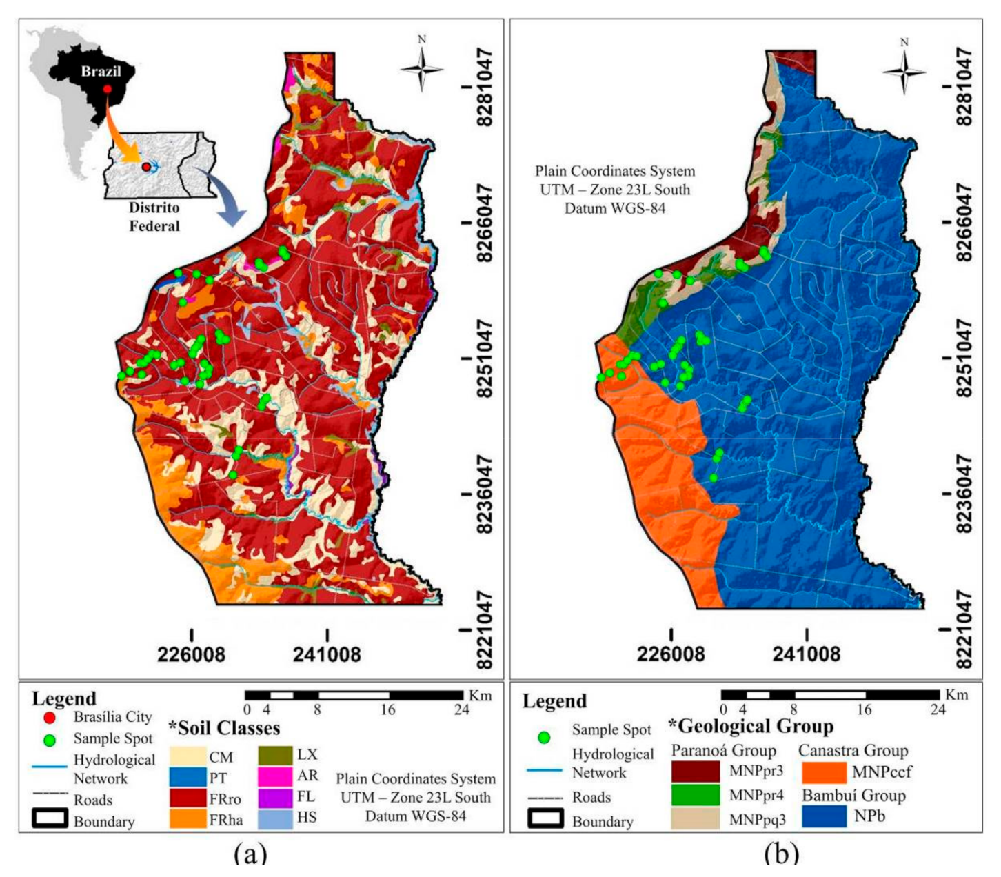
2.1. Study Area

The study area is located in the Eastern FD, between the UTM coordinates of 216,027 mE to 253,131 mE and 8,284,507 mN to 8,223,851 Mn, 23S zone (Figure 1a), covering an area of approximately 132,525 ha. The elevation varies from 800 m to 1200 m. According to Köppen’s classification system [18], the dominant type of climate is Cwa, that is, dry winter and hot summer. The mean annual precipitation ranges from 1200 mm to 1800 mm, mostly from the rainy season (from October to April) [19].

The study area is located in the Brazilian Central Plateau [20], presenting three geomorphological surfaces: a high plateau, intermediate plain surface, and dissected valley [21]. The terrain ranges from gentle-wavy to wavy relief [21], comprising 22.5% of the Rio Preto basin, a São Francisco River tributary. Sano et al. [22] stated the region belongs to the Cerrado (tropical savanna) biome. It is currently under intense agricultural exploitation, mainly for grain production, in a no-tillage management system [19].

The main source of soil maps was produced by Embrapa in 2004 [3] at a scale of 1:100,000 (Figure 1a). Ferralsols is the dominant soil type, covering 85% of the region, followed by Arenosols and hydromorphic soils along the streams. Freitas-Silva and Campos [23] identified the following geological formations (Figure 1b): The Paranoá Group, constituted by metarrythmits and an alternation of quartzites; the Canastra Group (phyllites); and the Bambuí Group (carbonate rocks).

2.2. Soil Characterization and Classification

At first, we established pedomorphogeological relationships for the selection of representative toposequences of the study area. We selected 42 field locations for soil sampling, and the description followed the guide proposed by the United States Geological Survey (USGS) [25]. The profile characterization was based on the Brazilian Soil Classification System [26]. The soil units were converted to the legends proposed by Soil Taxonomy [27] and those proposed by the World Reference Base for soil resources [24].

For each of the 42 soil profiles, we collected three soil samples at two depths (0–15 cm and 80–100 cm), generating 252 soil samples, as described in [28,29,30], between October 2019 and January 2020. The soil replicates were composed to represent one sample per depth. The soil colors were identified based on the Munsell soil color chart [31].

The following soil chemistry attributes were obtained from the laboratory analysis: pH in H₂O using a pH meter in soil solution; exchangeable calcium (Ca²⁺), magnesium (Mg²⁺), and aluminum (Al³⁺) based on extraction with potassium chloride (KCl); exchangeable potassium (K⁺) from flame photometer; and exchangeable phosphorus by the Mehlich-I extractor technique. Based on these data, we calculated the sum of bases (SB = Ca²⁺ + Mg²⁺ + K⁺), potential acidity (H⁺ + Al³⁺), cation exchange capacity (CEC = SB + [H⁺ + Al³⁺]), base saturation (V = [SB/CEC] ∗ 100), aluminum saturation (m = Al³⁺/[Al³⁺ + SB] ∗ 100), and clay activity ([CEC ∗ 1000]/g·Kg⁻¹) [27,29].

The organic matter content (OM) was determinated through wet oxidation, to procedures described in [29]. In this study, there were no quantitative mineral analyses. Despite that, the minerals were assessed qualitatively by comparing their soil spectral signatures with reference data [11,17,20].

Regarding the physical attributes, we measured the soil texture was determined by the Bouyoucos densimeter method (volumetric flask) with clay dispersed using sodium hydroxide (NaOH) based on the principle that suspended matter (silt and clay) exerts a density to the liquid [32].

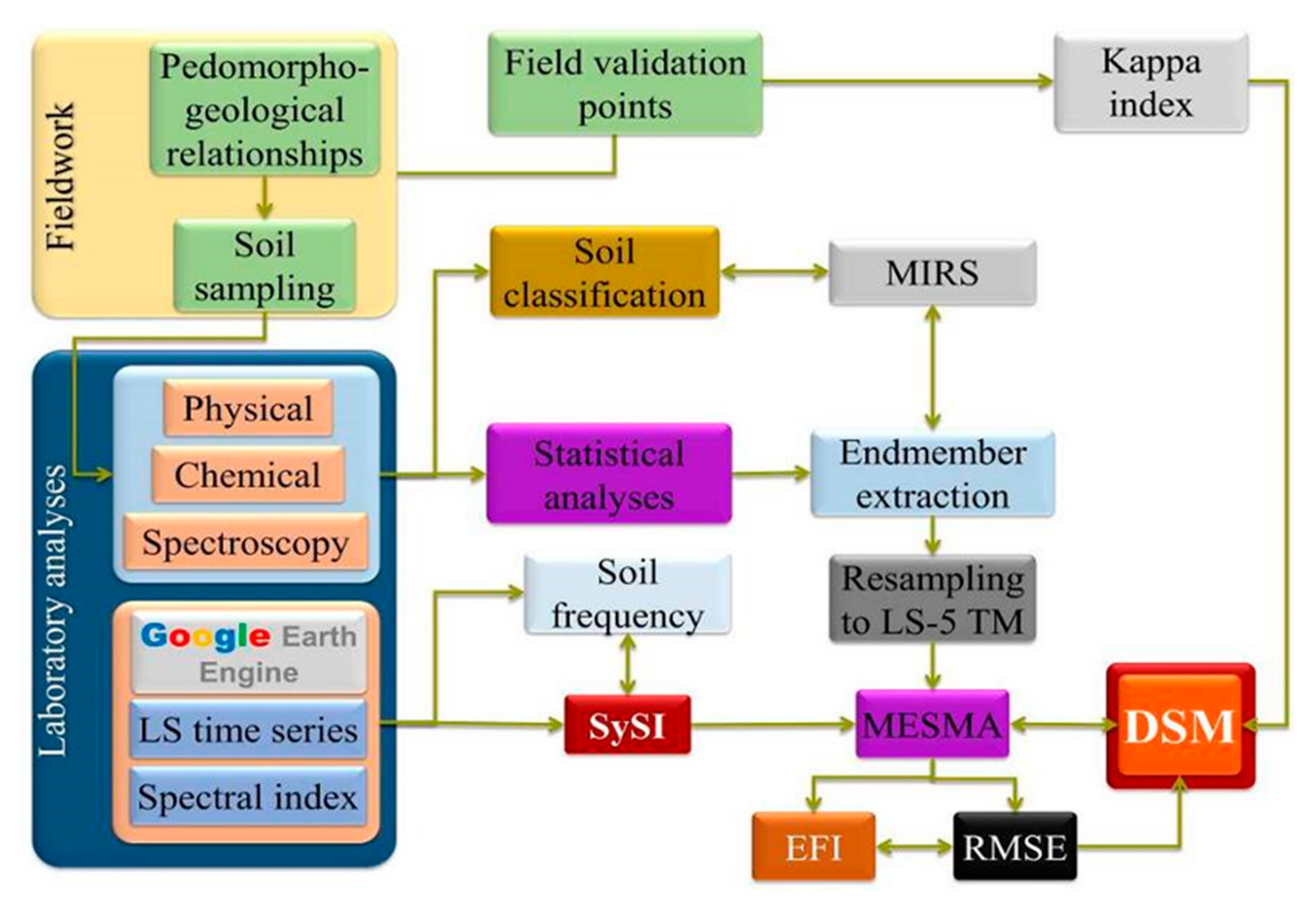
2.3. Data Processing

The main steps of the processing of the physical, chemical, and spectral soil data are shown in Figure 2. The physical and chemical attributes of the soil were analyzed using non-parametric statistics to produce soil endmembers. These soil endmembers were interpreted morphologically and resampled to six spectral band intervals of the Landsat 5 Thematic Mapper (TM) satellite.

Afterward, the reference spectra were inserted into the Multiple Endmember Spectral Mixture Analysis (MESMA) model, together with the denominated synthetic soil/rock image (SySI) created by [16] using cloud-computed processing of the Landsat time series [16] to produce the DSM from the study area. The modeling performance was assessed using the ground truth data collected in the field and the Kappa index and confusion matrix.

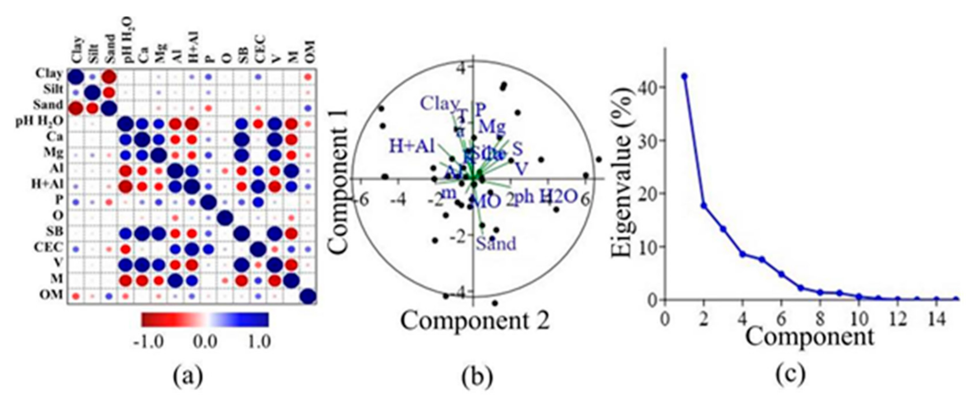
2.3.1. Statistical Analysis

We used descriptive statistics to compare our soil characteristics with other previous studies in the literature. We then employed the following non-parametric statistical techniques: Pearson’s correlation and principal component analysis (PCA) [33,34]. PCA is often used to determine the soil attributes that better explain the dataset and reduce the data dimensionality [10].

After, we selected the clay content as the soil grouping criterion through hierarchical cluster analysis (HCA) based on the single linkage clustering method and the Euclidean distance similarity index. The single linkage algorithm was chosen due to its capacity to process continuous datasets (in this case, a soil texture) [11].

2.3.2. Spectroscopy and Compilation of the Soil Spectral Library

We employed the FieldSpec 4 Pro spectroradiometer [35], which operates in the range of the electromagnetic spectrum, from visible to shortwave infrared (SWIR) (0.35 to 2.5 µm), to obtain reflectance data from the 42 air-dried and sieved soils sampled at the 0–15 cm depth, according to the standard procedures and geometric arrangement of the equipment described in [36]. Reflectance was measured at three different angles (45°, 90°, and 135°) [35] and converted into one reading by the simple average. Next, the percentages of clay, silt, and sand were correlated with the soil reflectance to find the best spectral bands to assess soil texture.

Following, we calculated the median of the spectral classes grouped by soil texture using HCA. The resulting curve represented the reference member of that soil class (endmember). Then, we interpreted the endmember’s spectral signature according to the general morphology (overall reflectance in the spectra) and the presence of specific absorption features in different wavelengths, according to the procedure described in [37]. Then, we subjected the reference spectra to the 2nd Kubelka-Munk derivative technique, which standardizes the reflectance values around an axis [38], allowing for a better observation of the target spectral behavior (Equation (1)).

$$\frac{k}{s}=\frac{{\left(1-R_{\infty }\right)}^2}{2R_{\infty }}=F\left(R_{\infty }\right)$$

(1)

where s corresponds to the scattering coefficient; k is the sample absorption coefficient; R_∞ is the diffuse reflectance; and F(R_∞) is the Kubelka–Munk function. Thus, we applied the Kubelka-Munk derivative function on spectral data to obtain patterns at specific diffuse reflectance peaks in the visible-near infrared (VNIR) and shortwave (SWIR) interval. The reflectance factors in the optical range of wavelengths, under this derivative, were submitted to Pearson’s correlation with the soil attributes.

We also correlated the clay, silt, and sand contents of 42 samples from the studied soil surface horizons with the reflectance factor distributed along the 2150 bands of the Fieldspec 4 Pro spectroradiometer [35]. The representative spectra were resampled according to the spectral bands of the Landsat 5 TM satellite [15].

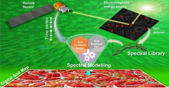
2.3.3. Landsat Time Series and Synthetic Soil/Rock Image

We edited a script using command-line programming in the Google Earth Engine (https://code.earthengine.google.com) (GEE) platform, a virtual environment for spatial and temporal data processing and analysis. The script returned a Landsat time series from 1984 to 2020. The Landsat collection of surface reflectance at Level 2 processing was employed. The median of pixels from the overlapping layers along the Landsat time series formed a synthetic image.

The algorithm generated a standard image based on the Landsat 5 TM band intervals: B1 (0.45–0.52 µm), B2 (0.52–0.60 µm), B3 (0.63–0.69 µm), B4 (0.76–0.90 µm), B5 (1.55–1.75 µm), and B7 (2.08–2.35 µm) [15]. As stated in [10,16,17], the algorithm uses spectral indices to remove clouds, vegetation, and burned areas, so that only bare soil/rock, water body, and urban area features remain in the time series. The water bodies and urbanized areas were removed from the analysis by masking.

Thus, we obtained a SySI image composed of the bare soil features’ median values throughout the time series. The seasonal differences on the surface reflectance were standardized during the synthetic image production process [16]. We also obtained the denominated Bare Soil Frequency or Soil Frequency Image (SFI) created by [16], which consists of the number of times that bare soil/rock features passed through filters established in the algorithm along the time series.

2.4. Soil Spectral Modeling and DSM Generation

MESMA [39] was employed to model the spectral mixture presented in SySI. The reference spectra were inputted into the model using the ENVI v. 5.3.1 software. MESMA is an algorithm available in the VIPER Tools application package and allows for the simultaneous analysis of several endmembers through automatic combinations, choosing the model with the lowest root mean square error (RMSE) [40].

As a result, we obtained an endmember fraction image (EFI), representing the proportion of pixels modeled, an image with the distribution of the errors (RMSE), and an image with endmember models, corresponding to our DSM map.

Gleisol and Histosol were excluded from the spectral modeling, since they are mostly covered by perennial vegetation. We also excluded the Haplic Plinthosol and Dystric Arenosol, since they are not spatially representative [3,10] or occur in locations that are difficult to capture using the method adopted in this study.

However, these soil classes were included in the clustering analysis to assess the grouping performance [11]. After the modeling, the spectral unmixing image was smoothed by a median filter (5 × 5), converted to the shapefile format, and assigned contrasting colors, as reported in [27].

Validation of Soil Spectral Mapping

We selected 328 points, which were distributed randomly and proportionally in the study area. Weights were assigned according to each polygon area [41]. The ground truth data were used to estimate the DSM map’s accuracy through a confusion matrix and the Kappa index [41,42].

3. Results

3.1. Soil Characteristics

The pedomorphogeological relationships analysis allowed us to select eight toposequences located in the central part of the study area. The 42 soil profiles were considered to be representative of the study area’s pedological distribution, as corroborated by field observations, the regional soil database, and previous findings [3,10,11,20]. The results of the textural and chemical soil analysis are shown in

Table 1. Descriptive statistics of the studied surface soil attributes.

Attributes/Parameters	Clay	Silt	Sand	pH	Al3+	SB	CEC	V	m	5 OM
	g·Kg−1				------ Cmolc·dm−3------			------ % ------		g·Kg−1
	Surface Horizons (0–20 cm)
Average	504.7	197.4	298.0	4.9	1.2	1.9	9.0	22.3	37.8	34.1
Standard error	31.3	20.1	40.3	0.1	0.2	0.2	0.3	2.5	4.4	1.1
Median	590.7	159.4	190.8	4.9	1.0	1.6	8.7	18.5	31.0	31.5
Mode	792.2	87.1	120.7	5.0	0.4	3.9	14.6	6.2	89.0	44.0
SD	202.7	130.4	261.3	0.6	1.2	1.3	2.1	16.4	28.5	7.4
Variance	41,102.1	17,008.2	68,259.4	0.4	1.4	1.7	4.3	267	814	55
Kurtosis	−0.2	−1.1	0.4	2.5	0.5	1.2	1.0	3.3	−0.9	−1.4
Asymmetry	−0.8	0.4	1.4	0.7	1.2	1.2	1.0	1.7	0.6	0.4
Range	747.3	442.5	863.5	3.1	4.1	5.3	8.8	76.3	89.0	24.0
Minimum	44.9	10.5	67.3	3.7	0.0	0.4	5.9	4.1	0.0	22.0
Maximum	792.2	453.0	930.8	6.8	4.1	5.7	14.6	80.4	89.0	46.0
Count	42.0	42.0	42.0	42.0	42.0	42.0	42.0	42.0	42.0	42.0
CL (90.0%)	52.6	33.9	67.8	0.2	0.3	0.3	0.5	4.2	7.4	1.9

Al³⁺: Exchangeable aluminum; SB: Sum of bases; CEC: Cation exchange capacity; V: Base saturation; m = Saturation by aluminum; OM: Organic matter; SD: Standard deviation; and CL: Confidence level.

.

The soil attribute data indicated soils with a clayey texture (average of 504.7 g·Kg⁻¹ of clay content), acid pH (average of 4.9), and high Al³⁺ levels (average of 37.8%) [24,26,27], characteristics inherited from the parent material that is, pelitic rocks [20]. The V average was below 22.3, which is typical of dystrophic soils, with a low natural fertility and highly weathered tropical soils [10]. This value is below that recommended for most commercial crops, which can be circumvented by soil management [43].

The OM levels were within average (34.1 g·Kg⁻¹) [11], as most of the sampling areas were covered by natural vegetation or within no-tillage systems, with straws covering the soil surface during certain periods [20,43].

Table 2. Descriptive statistics of the studied subsurface soil attributes.

Attributes/Parameters	Clay	Silt	Sand	pH	Al3+	SB	CEC	V	m	5 OM
	g·Kg−1				------ Cmolc·dm−3------			------ % ------		g·Kg−1
	Surface Horizons (0–20 cm)
Average	553.1	204.7	242.2	5.1	1.3	0.7	4.9	15.9	39.8	20.0
Standard error	29.8	19.1	35.6	0.0	0.3	0.1	0.3	1.4	5.1	1.3
Median	607.5	189.2	144.7	5.0	0.4	0.6	4.5	13.9	31.0	19.0
Mode	748.2	107.1	144.7	4.9	0.1	0.4	4.9	8.0	17.0	20.0
SD	193.2	123.9	230.6	0.3	1.7	0.4	2.2	8.9	32.9	8.2
Variance	37,325.8	15,361.9	53,194.3	0.1	2.9	0.2	4.8	79.8	1079.3	66.9
Kurtosis	0.0	−1.1	1.1	7.3	1.7	4.1	8.2	7.3	−1.4	−0.3
Asymmetry	−1.0	0.5	1.5	1.9	1.5	2.0	2.3	2.4	0.5	0.6
Range	715.3	386.6	845.1	1.6	6.5	1.7	12.2	44.3	93.0	29.0
Minimum	69.2	48.8	36.9	4.6	0.0	0.4	2.3	7.7	0.0	8.0
Maximum	784.6	435.3	882.0	6.2	6.5	2.1	14.5	52.0	93.0	37.0
Count	42.0	42.0	42.0	42.0	42.0	42.0	42.0	42.0	42.0	42.0
CL (90.0%)	50.2	32.2	59.9	0.1	0.4	0.1	0.6	2.3	8.5	2.1

Exchangeable aluminum (Al³⁺); SB: Sum of bases; CEC: Cation exchange capacity; V: Base saturation; m: Saturation by aluminum; OM: Organic matter; SD: Standard deviation; CL: Confidence level.

presents the soil attribute values. The lower OM and exchangeable base contents are consequences of no-tillage soil management, as demonstrated in [20]. The clayey texture presented little variations in the study area. The subsurface horizons normally present a lower V than surface layers due to fertilization practices and OM, which is concentrated up to a depth of 20 cm.

3.1.1. Statistical Analysis

The Pearson’s correlation among the 15 soil attributes expressed a strong relationship between clay, silt, and sand in the diagnostic horizons (Figure 3a). A strong positive correlation was found between the exchangeable bases and pH in H₂O, whereas the Al³⁺ values showed a strong negative correlation with pH in H₂O. The correlation results close to −1 or +1 were generally caused by redundant values: collinear variables derived from the attribute values, for example, the sum of the base and Ca²⁺ content. The PCA demonstrated the interaction between the attributes. Emphasis was placed on the attributes related to soil texture (Figure 3b). The eigenvalues indicated that the four components (sand, clay, V, and OM) could predict 80% of the dataset (Figure 3c).

The correlation results close to −1 or +1 were generally caused by redundant values: collinear variables derived from the attribute values, for example, the sum of the base and Ca²⁺ content. The PCA demonstrated the interaction between the attributes. Emphasis was placed on the attributes related to soil texture (Figure 3b). The eigenvalues indicated that the four components (sand, clay, V, and OM) could predict 80% of the dataset (Figure 3c).

The Pearson’s correlation between the texture and the spectra of the surface horizons (Figure 4a) showed a variation along the VNIR-SWIR interval. The clay fraction showed a negative correlation at the beginning of the visible spectra and the end of the SWIR. In contrast, the sand fraction obtained a positive correlation in these wavelengths, agreeing with most of the literature results obtained using these bands to predict soil texture [2,6,7,8,12,14,37]. The HCA successfully grouped the 42 soil samples based on texture content. This statistical method organized the samples into 13 clusters through the Euclidean distance similarity index (Figure 4b).

3.1.2. Soil Classification

Previous studies revealed that soil color is a function of mineralogical composition, mainly iron oxides and OM content [2,11]. Soils with high levels of quartz and low levels of OM and iron oxides are related to lighter colors [6,8,14,44]. Hematite and goethite are the most common iron oxides in tropical regions [10]. These minerals often condition the soil color, as demonstrated in [17], in which it was concluded that hematite produces reddish tones and goethite, red-yellowish, and yellowish tones in the Cerrado soils.

Rhodic Ferralsols showed similar colors along the soil profiles, ranging from dark red (10R 3/6) to light brown (2.5YR 5/8). The Haplic Ferralsols also showed homogeneous colors along the soil profile, ranging from dark-brown (7.5YR 3/4) to light-brown (10YR 6/6). The Petric Plinthosols and Haplic Plinthosols showed colors varying from brownish (10YR 6/8) in the A horizon to red (10R 5/8) in the C horizon.

Regarding Dystric Regosols colors, they exhibited a transition between the A and C horizons: from dark reddish-brown (5YR 4/4) to reddish yellow (10YR 5/4) in the A horizons and dark red (10R 3/6) to reddish yellow (2.5YR 6/8) in the C horizon.

The Haplic Cambisols presented a gradual color transition between the A and Bi horizons. In the C horizon, the dominant color was reddish (10R 6/4). The Dystric Arenosols presented reddish colors (10YR 5/6). They were derived from quarzitic rocks associated with the parent material, which is rich in iron oxides [20]. The Haplic Gleisols showed a color gradation between the A and C horizons (grey-blue tones, from 10YR 4/2 to 2.5Y 8/2). The Haplic Histosols presented dark colors, from black to brown-yellowish (10YR) typical of OM in decomposition [10].

The soil texture is a parameter indicative of the state of soil weathering [6]. This attribute is one of the key parameters in soil classification [24,26,27].

Table 3. Classification of soils in the study area.

SiBCS	Soil Taxonomy	WRB FAO	T	S	EM
Latossolo Vermelho Distrófico típico	Rhodic Acrustox	Dystric Rhodic Ferralsol	clayey	5	FRro-I
			v. clay.	2	FRro-II
Latossolo Vermelho-Amarelo distrófico típico	Typic Acrustox	Dystric Haplic Ferralsol	l. clay.	5	FRha-I
			clayey	6	FRha-II
Plintossolo Pétrico concrecionário típico	Petroferric Ustox	Dystric Petric Plinthosol	clayey	4	PTpt-I
			v. clay.	4	PTpt-II
Plintossolo Háplico distrófico típico	Typic Plinthaquox	Dystric Haplic Plintosol	v. clay.	2	PTha
Neossolo Regolítico distrófico típico	Typic Ustorthent	Dystric Regosol	clayey	2	RGdy-I
			v. clay.	4	RGdy-II
Gleissolo Háplico Tb distrófico típico	Typic Fluvaquents	Dystric Haplic Gleysol	clayey	2	GLha
Organossolo Háplico hêmico típico	Typic Haplohemist	Hemic HaplicHistosol	clayey	1	HSha
Cambissolo Háplico Tb distrófico típico	Oxic Dystrustepts	Dystric Rhodic Cambisol	clayey	3	CMdy
Neossolo Quartzarênico órtico típico	Typic Quartzipzament	Dystric Rhodic Arenosol	sandy	2	ARdy

SiBCS: Brazilian Soil Classification System [26]; WRB: World Reference Base [24]; T: Soil Texture, v. clay.: very clayey; l. clay.: loam-clayey; S.: Sample number; EM: Endmember.

shows nine soil units and 13 taxons, achieving the 5th categorical level, according to SiBCS [26], with texture as the key attribute.

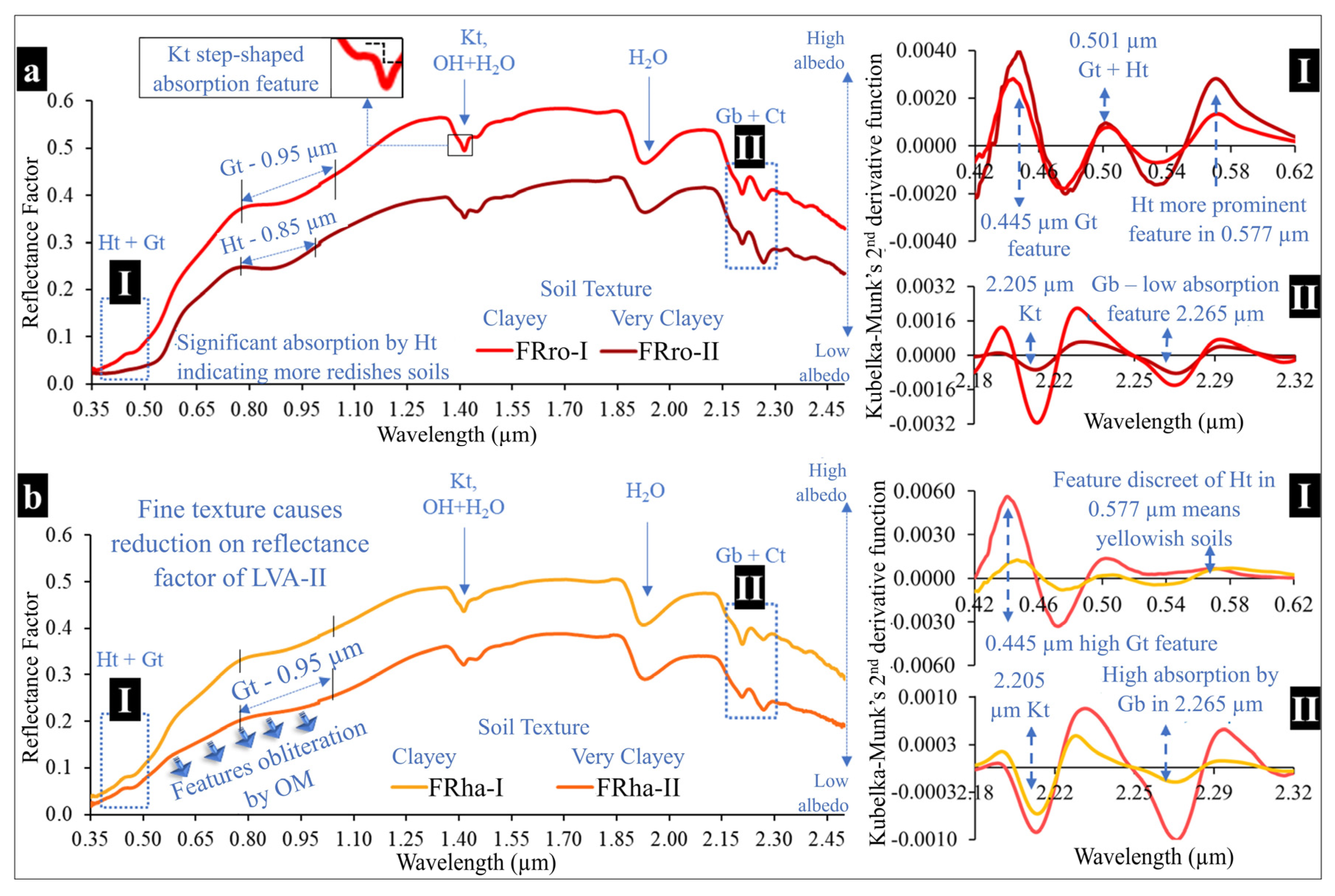
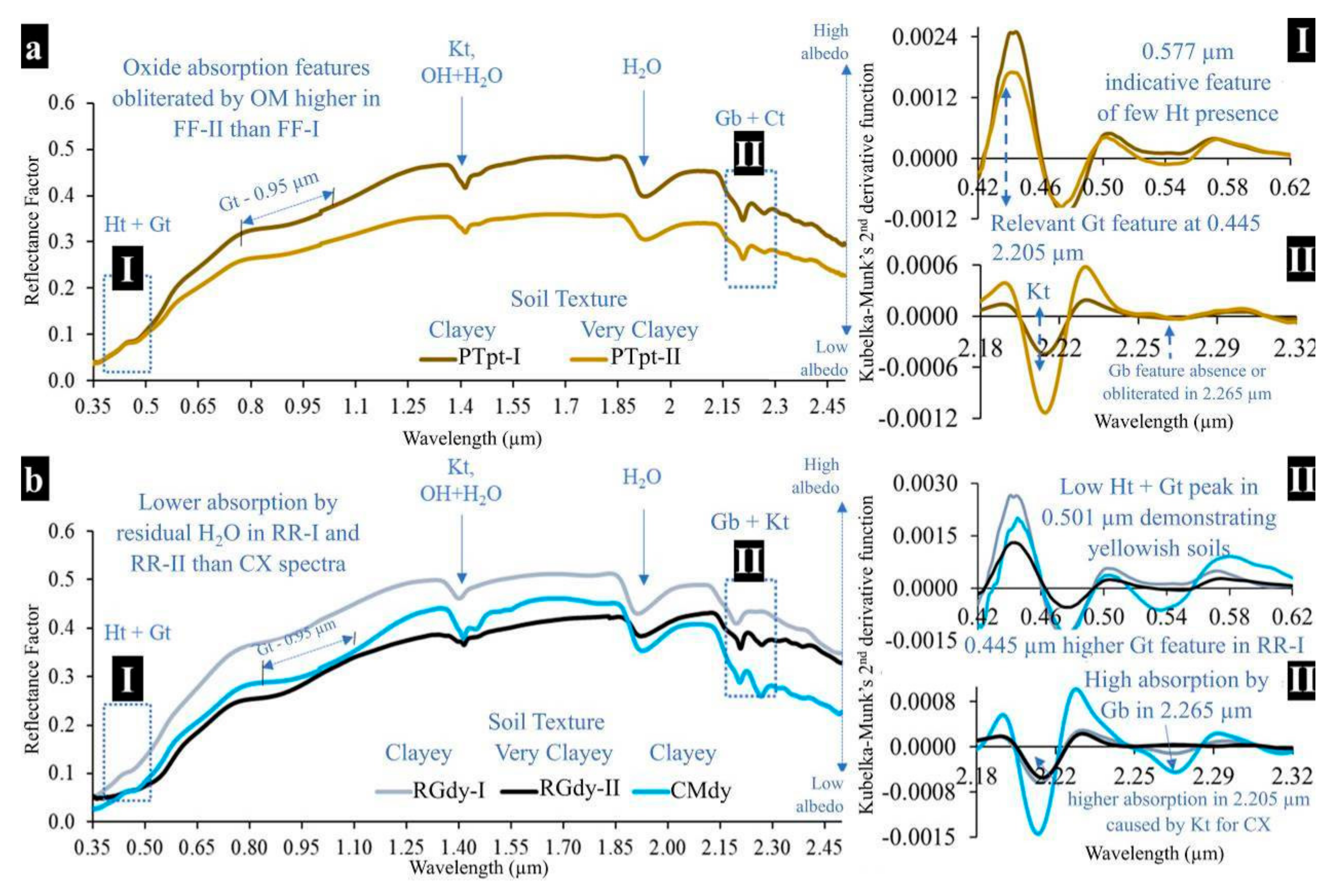
3.1.3. Soils Spectral Behavior

The spectral curves revealed an ascending pattern between 0.35 µm and 1.30 µm, changing to a flattened aspect in the range of 1.30 µm to 1.85 µm and decreasing between 1.85 µm to 2.50 µm. This spectral pattern represents the typical behavior of highly weathered Cerrado soils [6,10,11]. FRro-I, FRro-II, FRha-I, FRha-II, PTpt-I, PTpt-II, RGdy-I, RGdy-II, and CMdy showed similar results described in [10]. The OM content tends to reduce the reflectance factor [4,14,44]. Conversely, smaller soil particles increase the reflectance factor [6].

The FRro spectra showed a general curve aspect that is similar to the spectral signatures from the FRha (Figure 5). However, the reflectance factor for FRro was higher compared with FRha. The hematite features were more prominent in the FRro than the goethite features were more prominent in the FRha curves. These soils are more gibbsitic than the FRro. The FRro-I presented stronger absorption features than FRro-II due to the smaller particle size in the first endmember, especially those related to kaolinite features.

Baptista and Teobaldo [45] examined iron oxides in the region using spectroscopy, and they found hematite percentages ranging from 0 to 20%, gibbsite from 0.8 to 6.8% for tropical Rhodic Ferralsols. These results agree with [3], who state that iron oxide content varies by 15% in the study area. Lacerda and Barbosa [20] also analyzed soils in the same region. They observed significant differences in the mineral composition between FD soil classes since more evolved soil presented higher iron oxide contents and lower primary mineral contents than less weathered soils.

The authors from [37] successfully predicted mineralogical, physical, and chemical attributes from soil spectra and concluded that soil composition strongly affects the spectral signature of tropical soils. These authors also observed a range of iron oxides percentage varying from 0.2 to 24.1%, which directly influences the soil color in soils on basaltic rocks from Southern Brazil.

Figure 5 also reveals some differences in the Ferralsol spectra, mainly in the reflectance factor’s intensity. The OM had a more significant influence on FRha than FRro. The lower reflectance in this soil is also caused by the higher residual moisture presented by FRha. In this case, they present a subsurface layer of petroplinthite, which obstructs the water percolation along the soil profile [20].

The PTpt curve (Figure 6a) displayed a maximum reflectance factor of 0.35 in PTpt-I and 0.5 in PTpt-II. This spectral behavior is influenced by the very clayey texture, which is associated with the attenuating effect of OM on the PTpt-I curve [11]. It was possible to observe iron oxide features at specific points on the curve, with a predominance of goethite over hematite, in addition to kaolinite absorption features (1.4 µm and 2.205 µm), hydroxyl groups (1.4 µm and 1.9 µm), and gibbsite (2.265 µm). Previous studies [10,17,20,45] revealed that the soil mineral composition, which has a low content of primary minerals and a high content of oxides, indicates a high degree of weathering processes influencing soil colors.

Hydromorphic soils usually exhibit a lower albedo due to the higher OM and residual moisture in the soil solution [4]. These materials absorb a large part of electromagnetic energy, reducing the reflectance, especially in natural environments [37]. Opaque minerals in soils, such as iron oxides, also reduce the soils’ ability to reflect [6,13].

Figure 6b shows that the RGdy median spectra had a reflectance factor between 0.4 (RGdy-II) and 0.5 (RGdy-I). Despite the fine texture, the most significant albedo in these soils was due to the lower OM content, combined with stable minerals, such as quartz. Fe oxides exhibited the lowest absorption peaks, mainly in RGdy-I, as observed in [9]. The Regosols presented low absorption peak features of kaolinite and gibbsite, revealing the initial stage of pedoevolution [20].

By definition, CMdy are soils with an intermediate level of evolution [20]. They were represented by a single endmember, which reached the reflectance factor’s maximum intensity (0.45). The obliterating effect of the presence of OM in the soil was less significant than in the RGdy spectra. In agreement with the results presented in [44], the mineral features in CMdy are highlighted, especially the proportion between goethite and hematite and between kaolinite and gibbsite (Figure 6b). Our CMdy spectral curve indicated a weak presence of the 2:1 mineral. Poppiel et al. [10] attributed this spectral behavior to the OM content obliterating the mineral features.

As shown in Figure 6, the reflectance factors vary from 0.4 (RGdy-II) to 0.5 (RGdy-I) due to the different textures. The most significant albedo in these soils is related to the lower OM content, combined with stable minerals, such as quartz. Iron oxides exhibited the lowest absorption features, mainly in RGdy-I, as observed in [10]. The Regosols presented low absorption features of kaolinite and gibbsite, revealing the initial stage of pedoevolution [11].

3.2. Synthetic Soil/Rock Image Analysis

The SFI image is shown in Figure 7a. The bare soil/rock features registered by the algorithm, which varied from 0 to 461 times along the time series, are shown. The absence of bare soil features in some regions of the study area indicates the natural preservation areas, where the vegetation covers the soil during most of the year. The light grey areas show the consolidated agricultural plantations. A no-tillage agricultural system keeps the soil exposed in the off-season when the straws are almost all decomposed [43].

The SySI image (Figure 7b), a bare soil composite image, presented different purple tones, representing clayey soils, and light magenta tones, representing a sandy texture. Areas with a rough terrain also presented a low reflectance (dark tones close to purple). The SWIR reflectance was higher in flat landscapes than in rough terrains.

The sum of these factors caused a general reduction in the reflectance, highlighting the blue band (Red) over the red band (SWIR) in the Landsat TM RGB composition [16] and thus exhibiting a magenta color. Areas with dark colors were covered by sparse native vegetation, which periodically exposes the soils as permanently preserved areas [11]. Darker tones are also caused by successive burnings [7], typical in the Cerrado [22] along the time series considered in this research.

Bare soils covered 80% of the study area, mainly due to the no-tillage system, which has been widely adopted in the central region of Brazil [43] and is associated with the Cerrado climate, which presents a dry season and low relative humidity favoring natural soil exposure in sparse areas of Cerrado and areas in the Cerrado with a lot of shrubbery (savanna formation) [22].

Table 4. A list of some studies used the SySI method.

Authors	Study Area	Time Series	Percentage (%)
[5]	Swiss Plateau	1984–2016	43
[7]	Brazil, Southeast	1984–2011	68
[8]	Brazil, Southeast	1984–2017	53
[9]	Germany	1984–2014	26
[10]	Brazil, Midwest	1984–2018	74
[16]	Brazil, Southeast	1984–2018	68
[17]	Brazil, Midwest	1984–2019	100 *
[46]	Worldwide	1985–2015	34

* Using Krigagem on the achieved SySI area.

lists some authors who also applied a similar method.

3.3. Mapped Area Accounting

We obtained 106,828 ha (80.6% of the total area) of the study area (

Table 5. Accounting for mapped and unmapped areas. WRB: World Reference Base [24].

Mapping Unit	Soil Class on WRB System [24]	Area
		Hectares	Percentage (%)
FRro-I	Dystric Rhodic Ferralsol (Clayic)	53,754	50.3
FRro-II	Dystric Rhodic Ferralsol (Very Clayic)	15,149	14.2
FRha-I	Dystric Haplic Ferralsol (Loam-Clayic)	5051	4.7
FRha-II	Dystric Haplic Ferralsol (Clayic)	12,301	11.5
PTpt-I	Dystric Petric Plinthosol (Clayic)	4844	4.5
PTpt-II	Dystric Petric Plinthosol (Very Clayic)	10,252	9.6
RGdy-I	Dystric Regosol (Clayic)	1424	1.3
RGdy-II	Dystric Regosol (Very Clayic)	3,223	3.0
CMdy	Dystric Haplic Cambisol (Clayic)	828	0.8
Subtotal		106,828	80.6
Unmapped		25,697	19.4
Total		132,525	100.0

), which corresponds to the pixels captured using the SySI methodology over the time series. FRro and FRha were the dominant soil types (80%), followed by PTpt and RGdy. CMdy presented a low spatial representation. CMdy generally occurs in transition zones associated with FRha and PTpt. These results are in agreement with previous studies reported in [3,10] regarding soil classes proportion and distribution.

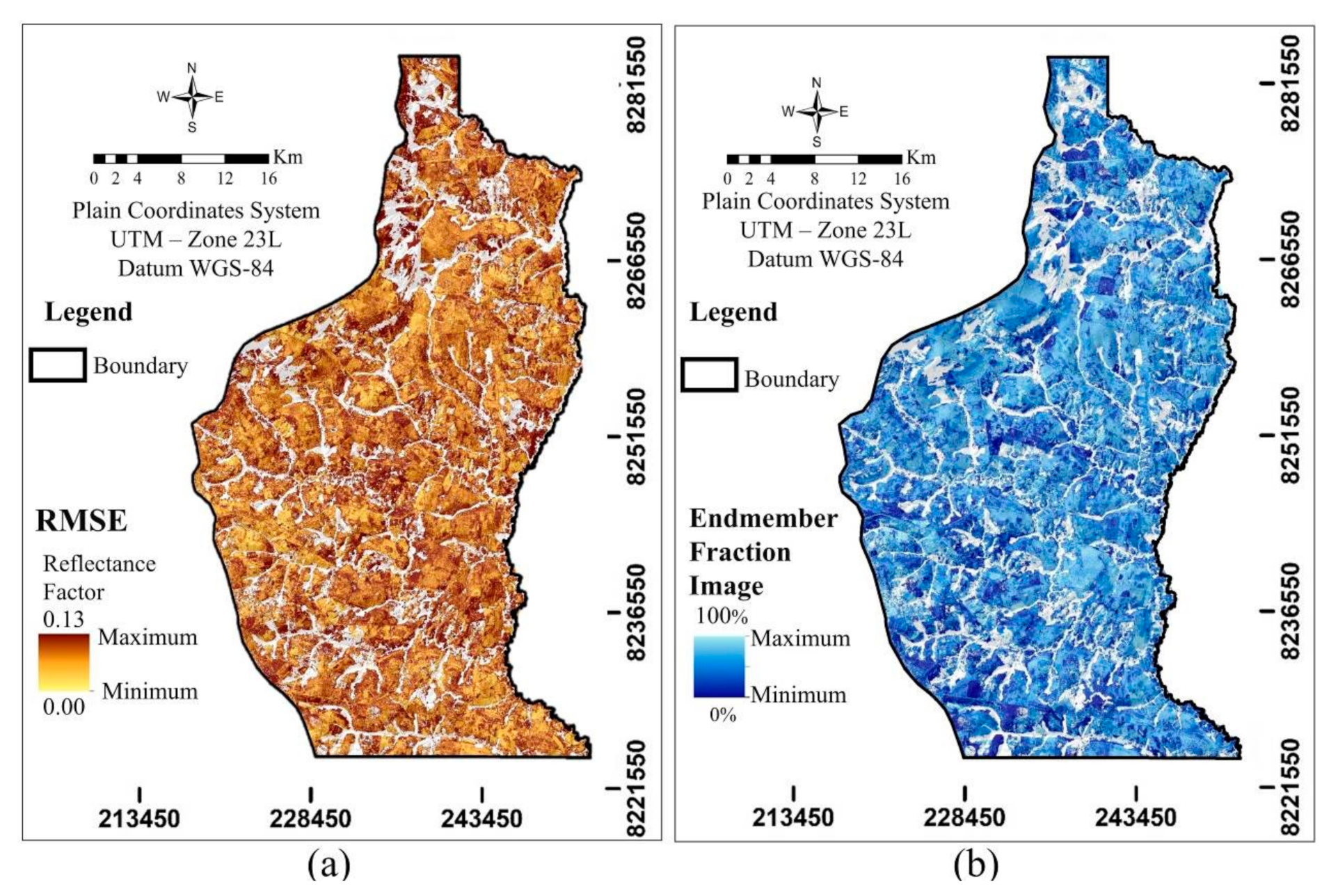
3.4. Validation of Spectral Mixing Models

The DSM accuracy evaluation, based on the analysis of 328 validation points, presented a Kappa index of 0.74 (

Table 6. Confusion matrix for digital soil mapping.

Soil Classes		Field Truth									Total	UA	OE
		A	B	C	D	E	F	G	H	I		%
Digital soil map	A	79	5	2	2	1	0	0	0	1	90	88	12
	B	8	38	0	0	0	0	0	0	0	46	83	17
	C	1	0	17	2	0	0	0	1	1	22	77	23
	D	2	1	6	27	7	4	1	2	0	50	54	46
	E	1	2	0	7	23	3	1	1	1	39	59	41
	F	1	0	0	4	0	25	0	1	0	31	81	19
	G	0	0	0	2	5	2	19	1	0	29	66	34
	H	0	0	0	1	0	0	1	12	0	14	86	14
	I	0	0	0	1	1	0	0	0	5	7	71	29
Total		92	46	25	46	37	34	22	18	8	245
PA	%	86	83	68	59	62	74	86	67	63
CE		14	17	32	41	38	26	14	33	38
κ%		74.6951						Validation points				328

A: FRro-I; B: FRro-II; C: FRha-I; D: FRha-II; E: PTpt-I; F: PTpt-II; G: RGdy-I; H: RGdy-II; I: CMdy; UA: User’s accuracy; OE: Omission error; PA: Producer’s accuracy; CE: Commission error, κ: Kappa index, in percentage.

), which is considered a substantial agreement level, according to the classification proposed in [41,42]. The Producer’s Accuracy (PA) achieved the highest percentage for FRro-I and RGdy-I (86%). This means that these soils presented the best spectral separation, indicating that the method modeled these endmembers more correctly, with a higher number of matches than that achieved for other endmembers. The lowest scores of User’s Accuracy (UA) were found for FRha-II and PTpt-I (54% and 59%, respectively). The omission errors (OE) ranged from 12% (FRro-I) to 46% (FRha-I).

Still, regarding Table 6, we observed CMdy presenting 38% of the commission error (CO) due to the low number of validation points. As stated in [6], when PTdy samples are air-dried, crushed, and sieved, their spectral behavior becomes similar to that of FRro. This occurs because Ferralsol and Petric Plinthosol are similar in pedogenetic terms. In other words, they present ferratilization as one of their soil formation processes [20].

4. Discussion

4.1. Performance of Spectral Modeling

The MESMA method achieved 100% of the SySI, meaning that every pixel is associated with at least one endmember. The RMSE image showed the best and worst modeling fits (lowest and highest error, respectively) (Figure 8a), while the EFI exhibited the endmember’s proportion utilized to model the features (Figure 8b). The general performance of the MESMA can be considered satisfactory, according to the criterion described in [10], since it was able to model nine endmembers presenting low errors, which is also the criterion described in [1].

In Figure 8a, the light-yellow tones indicate low RMSE values, starting from 0, gradually changing to dark red tones, indicating the maximum values (0.13) of RMSE. The research proposed in [10] stated that the RMSE is a standard way to assess quantitative data predictive models. They also obtained lower error values (about 3%), attributing this performance to the small extension of the study area analyzed.

The low RMSE values were associated with the agricultural areas and a flat relief, while the high errors were related to the natural vegetation and rough terrain. This fact was attributed in [16] to the higher and lower spectral mixture in these areas, respectively. Genú et al. [1] demonstrated the same behavior, in which the endmember fraction image presented a lower endmember proportion in areas where there was a lower bare soil frequency.

As in [10], our global fraction of modeled endmembers was considered high, with an average proportion of 68%, meaning that the reference spectra reached approximately three of every four modeled pixels. This result was attributed to the representative soil spectral library, which could portray the spectral behavior dataset and a suitable soil clustering technique, similar to that employed in [1] for a similar study of bare soils in Southern Brazil.

Gallo et al. [8] also utilized HCA to group the soils in Southern Brazil and concluded that this method is able to predict several attributes using other similarity indices, for example, the complete linkage. Poppiel et al. [11] achieved similar findings when they grouped soils using the Munsell color as the cluster criterion in Midwest Brazil.

4.2. Digital Soil Map

The DSM map showed irregular polygons distributed along the entire study area (Figure 9). FRro occurred predominantly in areas with a flat relief and high elevation, surrounded by very clayey FRro at lower levels [20], while FRha appeared in gentle-wavy slopes, which are usually associated with FRro and PTpt. When the slope increases, CMdy, PTpt, and RGdy become dominant. FRha occurs at the plateau’s edges, which is in agreement with the parent material (quartzites) [20,22].

Some soil classes in the agricultural areas showed regular polygons. These areas are related to the dominant agricultural practices in the study area [11]. Traditional or no-tillage practices influenced the reflectance, leading the image presenting dark or light features in the SySI, thus confusing the models [10]. As reported in [16], the rectangular, triangular, or circular patterns in the map represent anthropized features.

We obtained a Kappa index of 0.74. The agreement coefficient demonstrated in [44] showed spectroscopic data and terrain attributes for mapping soil classes, obtaining a Kappa index of 0.41. In [9], the authors achieved a 0.75 Kappa index for the DSM in the same region of the current study. As stated in [8], these similar spectral behaviors led to errors in multispectral modeling

5. Conclusions

The MESMA algorithm-based spectral classification was efficient in the discrimination of the soil spectral patterns in the study area. It had a strong capacity to identify the most suitable soil class (endmember) for every pixel in the synthetic soil/rock image, with few errors. This fact explains the satisfactory accuracy of the digital soil map generated in this study. However, spectral libraries of endmembers with a low spatial representativity could lead to confusion in the modeling process.

We assume that the percentages of bare soils will increase over time by expanding the Landsat legacy and integrating other sensors. A more robust time series could provide data that would improve the modeling performance. Additionally, the hybrid mapping could supply unmapped areas using geostatistical techniques applied, for example, in pedometry. Alternatively, we could include spectral information to implement new predictive models or increase the capacity of the existing ones.

Although the proposed method demonstrated efficiency for digital soil mapping in the study area, differences in the pedomorphogeological and vegetation cover conditions must be taking into consideration for application of this method in other regions. Besides, the MESMA has a limited number of endmembers, which may be another challenging issue in extrapolating to other regions.

References

1. Genú, A.M.; Roberts, D.; Demattê, J.A.M. The use of multiple endmember spectral mixture analysis (MESMA) for the mapping of soil attributes using ASTER imagery. Acta Sci. 2013, 35, 377–386. [Google Scholar] [CrossRef] [Green Version]
2. Chabrillat, S.; Ben-Dor, E.; Cierniewski, J.; Gomez, C.; Schmid, T.; van Wesemael, B. Imaging spectroscopy for soil mapping and monitoring. Surv. Geophys. 2019, 40, 361–399. [Google Scholar] [CrossRef] [Green Version]
3. Reatto, A.; Martins, E.S.; Farias, M.F.R.; Silva, A.V.; Carvalho, O.A., Jr. Mapa Pedológico Digital: SIG Atualizado do Distrito Federal Escala 1:100.000 e uma Síntese do Texto Explicativo; (Documentos, 120); Embrapa Cerrados: Planaltina, Brazil, 2004; p. 31. [Google Scholar]
4. Ben-Dor, E.; Chabrillat, S.; Demattê, J.A.M.; Taylor, G.R.; Hill, J.; Whiting, M.L.; Sommer, S. Using imaging spectroscopy to study soil properties. Remote Sens. Environ. 2009, 113, 38–55. [Google Scholar] [CrossRef]
5. Diek, S.; Schaepman, M.E.; Jong, R. Creating multi-temporal composites of airborne imaging spectroscopy data in support of digital soil mapping. Remote Sens. 2016, 8, 906. [Google Scholar] [CrossRef] [Green Version]
6. Lacerda, M.P.C.; Demattê, J.A.M.; Sato, M.V.; Fongaro, C.T.; Gallo, B.C.; Souza, A.B. Tropical texture determination by proximal sensing using a regional spectral library and its relationship with soil classification. Remote Sens. 2016, 8, 701. [Google Scholar] [CrossRef] [Green Version]
7. Fongaro, C.T.; Demattê, J.A.M.; Rizzo, R.; Safanelli, J.L.; Mendes, W.S.; Dotto, A.C.; Vicente, L.E.; Franceschini, M.H.D.; Ustin, S.L. Improvement of clay and sand quantification based on a novel approach with a focus on multispectral satellite images. Remote Sens. 2018, 10, 1555. [Google Scholar] [CrossRef] [Green Version]
8. Gallo, B.C.; Demattê, J.A.M.; Rizzo, R.; Safanelli, J.L.; Mendes, W.S.; Lepsch, I.F.; Sato, M.V.; Romero, D.J.; Lacerda, M.P.C. Multi-temporal satellite images on topsoil attribute quantification and the relationship with soil classes and geology. Remote Sens. 2018, 10, 1571. [Google Scholar] [CrossRef]
9. Rogge, D.; Bauer, A.; Zeidler, J.; Mueller, A.; Esch, T.; Heiden, U. Building an exposed soil composite processor (SCMaP) for mapping spatial and temporal characteristics of soils with Landsat imagery (1984–2014). Remote Sens. Environ. 2018, 205, 1–17. [Google Scholar] [CrossRef] [Green Version]
10. Poppiel, R.R.; Lacerda, M.P.C.; Demattê, J.A.M.; Oliveira, M.P.; Gallo, B.C.; Safanelli, J.L. Soil class map of the Rio Jardim watershed in Central Brazil at 30 meter spatial resolution based on proximal and remote sensed data and MESMA method. Data Brief. 2019, 25, 104070. [Google Scholar] [CrossRef]
11. Poppiel, R.R.; Lacerda, M.P.C.; Demattê, J.A.M.; Oliveira, M.P.; Gallo, B.C.; Safanelli, J.L. Pedology and soil class mapping from proximal and remote sensed data. Geoderma 2019, 348, 189–206. [Google Scholar] [CrossRef]
12. Demattê, J.A.M.; Dotto, A.C.; Paiva, A.F.S.; Sato, M.V.; Dalmolin, R.S.D.; Araújo, M.S.B.; Silva, E.B.; Nanni, M.R.; ten Caten, A.; Noronha, N.C.; et al. The Brazilian Soil Spectral Library (BSSL): A general view, application and challenges. Geoderma 2019, 354, 113793. [Google Scholar] [CrossRef]
13. Liu, J.; Xie, J.; Han, J.; Wang, H.; Sun, J.; Li, R.; Li, S. Visible and near-infrared spectroscopy with chemometrics are able to predict soil physical and chemical properties. J. Soil Sediment. 2020, 20, 2749–2760. [Google Scholar] [CrossRef]
14. Coblinski, J.A.; Giasson, É.; Demattê, J.A.M.; Dotto, A.C.; Costa, J.J.F.; Vašát, R. Prediction of soil texture classes through different wavelength regions of reflectance spectroscopy at various soil depths. Catena 2020, 189, 104485. [Google Scholar] [CrossRef]
15. USGS. Landsat Data Users Handbook; EROS Center: Sioux Falls, SD, USA, 2019; 196p.
16. Demattê, J.A.M.; Fongaro, C.T.; Rizzo, R.; Safanelli, J.L. Geospatial Soil Sensing System (GEOS3): A powerful data mining procedure to retrieve soil spectral reflectance from satellite images. Remote Sens. Environ. 2018, 212, 161–175. [Google Scholar] [CrossRef]
17. Poppiel, R.R.; Lacerda, M.P.C.; Safanelli, J.L.; Rizzo, R.; Oliveira, M.P., Jr.; Novais, J.J.; Demattê, J.A.M. Mapping at 30 m Resolution of Soil Attributes at Multiple Depths in Midwest Brazil. Remote Sens. 2019, 11, 2905. [Google Scholar] [CrossRef] [Green Version]
18. Köppen, W. Klassifikation der Klimate nach Temperatur, Niederschlag und Jahresablauf (Classification of climates according to temperature, precipitation and seasonal cycle). Petermanns Geogr. Mitt. 1918, 64, 193–203. [Google Scholar]
19. Castro, K.B.; Lima, L.A.S. Atlas do Distrito Federal; CODEPLAN: Brasília, Brazil, 2020. [Google Scholar]
20. Lacerda, M.P.C.; Barbosa, I.O. Relações pedomorfológicas e distribuição de pedoformas na estação ecológica Águas Emendadas, Distrito Federal. Rev. Bras. Cienc. Solo 2012, 36, 709–721. [Google Scholar] [CrossRef] [Green Version]
21. Pinto, M.N. Caracterização geomorfológica do Distrito Federal. In Cerrado: Caracterização, Ocupação e Perspectivas; Pinto, M.N., Ed.; UnB—SEMATEC: Brasília, DF, Brazil, 1994. [Google Scholar]
22. Sano, E.E.; Rodrigues, A.A.; Martins, E.S.; Bettiol, G.M.; Bustamante, M.M.C.; Bezerra, A.S.; Couto, A.F., Jr.; Vasconcelos, V.; Schüler, J.; Bolfe, E.L. Cerrado ecoregions: A spatial framework to assess and prioritize Brazilian savanna environmental diversity for conservation. J. Environ. Manag. 2019, 232, 818–828. [Google Scholar] [CrossRef] [PubMed]
23. Freitas-Silva, F.H.; Campos, J.E.G. Geologia do Distrito Federal. In Inventário Hidrogeológico e dos Recursos Hídricos Superficiais do Distrito Federal; Barros, J.C.B., Ed.; CAESB: Brasília, Brazil, 1987. [Google Scholar]
24. Schad, P.; van Huysteen, C.; Michéli, E. World Reference Base for Soil Resources 2014: International Soil Classification System for Naming Soils and Creating Legends for Soil Maps; FAO: Rome, Italy, 2014. [Google Scholar]
25. Ditzler, C.; Scheffe, K. (Eds.) Soil Survey Manual Agriculture. In USDA Handbook 18; Government Printing Office: Washington, DC, USA, 2017. [Google Scholar]
26. Santos, H.G.; Jacomine, P.K.T.; Anjos, L.H.C.; Oliveira, V.A.; Lumbreras, J.F.; Coelho, M.R.; Almeida, J.A.; Araújo Filho, J.C.; Oliveira, J.B.; Cunha, T.J.F. Sistema Brasileiro de Classificação de Solos; Embrapa Solos: Rio de Janeiro, Brazil, 2018. [Google Scholar]
27. USDA. Illustrated Guide to Soil Taxonomy (Version 2); USDA: Lincoln, NE, USA, 2015.
28. Schoeneberger, P.J.; Wysocki, D.A.; Benham, E.C. Field Book for Describing and Sampling Soils; Version 3.0; USDA: Lincoln, NE, USA, 2012.
29. Soil Survey Staff. Soil Survey Field and Laboratory Methods Manual; USDA, Natural Resources Conservation Service: Washington, DC, USA, 2014.
30. Teixeira, P.C.; Donagemma, G.K.; Fontana, A.; Teixeira, W.G. Manual de Métodos de Análise de Solo; Embrapa Solos: Rio de Janeiro, Brazil, 2017. [Google Scholar]
31. Munsell Color. Munsell Soil Color Book; Munsell Color: Grand Rapids, MI, USA, 2015. [Google Scholar]
32. Bouyoucos, G.J. Hydrometer method improved for making particle size analyses of soils 1. Agron. J. 1962, 54, 464–465. [Google Scholar] [CrossRef]
33. Chang, C.-W.; Laird, D.A.; Mausbach, M.J.; Hurburgh, C.R. Near-infrared reflectance spectroscopy—Principal components regression analyses of soil properties. Soil Sci. Soc. Am. J. 2001, 65, 480–490. [Google Scholar] [CrossRef] [Green Version]
34. Ogen, Y.; Zaluda, J.; Francos, N.; Goldshleger, N.; Ben-Dor, E. Cluster-based spectral models for a robust assessment of soil properties. Geoderma 2019, 340, 175–184. [Google Scholar] [CrossRef]
35. ASD Inc. ASD Fieldspec® 4: The Industry-Leading Portable Device for Field Spectroscopy, 6th ed.; ASD Inc.: Falls Church, VA, USA, 2019. [Google Scholar]
36. Romero, D.J.; Ben-Dor, E.; Demattê, J.A.M.; Souza, A.B.; Vicente, L.E.; Tavares, T.R.; Martello, M.; Strabeli, T.F.; Barros, P.P.S.; Fiorio, P.R.; et al. Internal soil standard method for the Brazilian soil spectral library: Performance and proximate analysis. Geoderma 2018, 312, 95–103. [Google Scholar] [CrossRef]
37. Demattê, J.A.M.; Bellinaso, H.; Romero, D.J.; Fongaro, C.T. Morphological Interpretation of Reflectance Spectrum (MIRS) using libraries looking towards soil classification. Sci. Agric. 2014, 71, 509–520. [Google Scholar] [CrossRef]
38. Scheinost, A.C.; Chavernas, A.; Barrón, V.; Torrent, J. Use and limitations of second-derivative diffuse reflectance spectroscopy in the visible to near-infrared range to identify and quantify Fe oxide minerals in soils. Clays Clay Miner. 1998, 46, 528–536. [Google Scholar] [CrossRef]
39. Roberts, D.A.; Gardner, M.; Church, R.; Ustin, S.; Scheer, G.; Green, R.O. Mapping chaparral in the Santa Monica Mountains using multiple endmember spectral mixture models. Remote Sens. Environ. 1998, 65, 267–279. [Google Scholar] [CrossRef]
40. Crabbé, A.H.; Jakimow, B.; Somers, B.; Roberts, D.A.; Halligan, K.; Dennison, P.; Dudley, K. Viper Tools Software. 2019. Available online: http://tools2019.innopolis.ru/ (accessed on 31 January 2021).
41. Congalton, R.G.; Green, K. Assessing the Accuracy of Remotely Sensed Data Principles and Practices, 2nd ed.; CRC Press: Boca Raton, FL, USA, 2013. [Google Scholar]
42. Landis, J.R.; Koch, G.G. The measurement of observer agreement for categorical data. Biometrics 2011, 33, 159–174. [Google Scholar] [CrossRef] [Green Version]
43. Sousa, D.M.G.; Lobato, E. Cerrado: Correção do Solo e Adubação; Embrapa: Brasília, Brazil, 2004. [Google Scholar]
44. Rizzo, R.; Demattê, J.A.M.; Lepsch, I.F.; Gallo, B.C.; Fongaro, C.T. Digital soil mapping at local scale using a multi-depth Vis-NIR spectral library and terrain attributes. Geoderma 2016, 274, 18–27. [Google Scholar] [CrossRef]
45. Baptista, G.M.M.; Teobaldo, D. WorldView-2 sensor for the detection of hematite and goethite in tropical soils. Pesq. Agrop. Brasileira 2017, 52, 1192–1202. [Google Scholar] [CrossRef] [Green Version]
46. Demattê, J.A.M.; Safanelli, J.L.; Poppiel, R.R.; Rizzo, R.; Silvero, N.E.Q.; de Sousa Mendes, W.; Bonfatti, B.R.; Dotto, A.C.; Salazar, D.F.U.; de Oliveira Mello, F.A.; et al. Bare Earth’s surface spectra as a proxy for soil resource monitoring. Sci. Rep. 2020, 10, 4461. [Google Scholar] [CrossRef]
Figure 1. Soil (a) and geological (b) maps of the study area. The soil map was adapted from the World Reference Base [24]. CM: Cambisols; PT: Plinthosols; FRro: Rhodic Ferralsol; FRha: Haplic Ferralsol; LX: Lixisol; AR: Arenosol; FL: Fluvisol; HS: Hydromorphic soils; MNPpr3: sandy metarrythmits; MNPpr4: clayey metarrythmits; MNPpq3: quartzite; MNPccf: carbonated phyllite; and NPb: pelitic rocks. Sources: [3,23].
Remotesensing 13 01181 g001
Figure 2. Flowchart of the methodology for the production of the digital soil map of the study area. MIRS: morphological interpretation of reflectance spectra [16]; LS: Landsat; LS-5 TM: Landsat 5 Thematic Mapper; DSM: digital soil map; EFI: endmember fraction image; RMSE: root mean square error; MIRS: morphological interpretation of reflectance spectra; and SySI: synthetic soil/rock image.
Remotesensing 13 01181 g002
Figure 3. Pearson correlation between soil attributes (a), principal component analysis (b), and eigenvalues (c) of the soil diagnostic horizons.
Remotesensing 13 01181 g003
Figure 4. (a) Pearson’s correlation between texture and spectral signatures; (b) texture-based hierarchical cluster analysis. FRro-I and FRro-II: Rhodic Ferralsol; FRha-I and FRha-II: Haplic Ferralsol; PTpt-I and PTpt-II: Petric Plinthosol; PTha: Haplic Plinthosol; RGdy-I, RGdy-II: Dystric Regosol; CMdy: Dystric Cambisol; GLha: Haplic Gleisol; HSha: Haplic Histosol; and ARdy: Dystric Arenosol.
Remotesensing 13 01181 g004
Figure 5. Interpretation of the spectral behavior of (a) Rhodic Ferralsol (FRro-I and FRro-II) and (b) Haplic Ferralsol (FRha-I and FRha-II). Ht: Hematite, Gt: Goethita; Kt: Kaolinite; Gb: Gibbsite; OM: Organic matter.
Remotesensing 13 01181 g005
Figure 6. Interpretation of the spectral behavior of (a) Petric Plinthosol (PTpt-I and PTpt-II) and (b) Dystric Regosol and Dystric Cambisol (RGdy-I, RGdy-II, and CMdy). Ht: Hematite; Gt: Goethita; Kt: Kaolinite; Gb: Gibbsite; and OM: Organic matter.
Remotesensing 13 01181 g006
Figure 7. (a) Soil frequency image of the Landsat time series and (b) synthetic soil/rock image.
Remotesensing 13 01181 g007
Figure 8. Image of (a) root mean square error (RMSE) and (b) fraction image from the modeled endmember.
Remotesensing 13 01181 g008
Figure 9. Digital soil map of the eastern Federal District, according to the World Reference Base [24]. FRro-I: Dystric Rhodic Ferralsol (clayic); FRro-II: Dystric Rhodic Ferralsol (very clayic); FRha-I: Dystric Haplic Ferralsol (clayic); FRha-II: Dystric Haplic Ferralsol (loam-clayic); PTpt-I: Dystric Petric Plinthosol (clayic); PTpt-II: Dystric, Petric Plinthosol (very clayic); RGdy-I: Dystric Regosol (very clayic); RGdy-II: Dystric Regosol (very clayic); and CMdy: Dystric Haplic Cambisol (clayic).
Remotesensing 13 01181 g009