Increasing Spatio-Temporal Resolution for Monitoring Alpine Solifluction Using Terrestrial Laser Scanners and 3D Vector Fields

Abstract

This article investigates the usage of terrestrial laser scanner (TLS) point clouds for monitoring the gradual movements of soil masses due to freeze–thaw activity and water saturation, commonly referred to as solifluction. Solifluction is a geomorphic process which is characteristic for hillslopes in (high-)mountain areas, primarily alpine periglacial areas and the arctic. The movement can reach millimetre-to-centimetre per year velocities, remaining well below the typical displacement mangitudes of other frequently monitored natural objects, such as landslides and glaciers. Hence, a better understanding of solifluction processes requires increased spatial and temporal resolution with relatively high measurement accuracy. To that end, we developed a workflow for TLS point cloud processing, providing a 3D vector field that can capture soil mass displacement due to solifluction with high fidelity. This is based on the common image-processing techniques of feature detection and tracking. The developed workflow is tested on a study area placed in Hohe Tauern range of the Austrian Alps with a prominent assemblage of solifluction lobes. The derived displacements were compared with the established geomonitoring approach with total station and signalized markers and point cloud deformation monitoring approaches. The comparison indicated that the achieved results were in the same accuracy range as the established methods, with an advantage of notably higher spatial resolution. This improvement allowed for new insights considering the solifluction processes.

1. Introduction

In the periglacial zones of high-alpine areas, the slow downslope movement of soil, induced by cyclic freezing and thawing, is a prevalent hillslope process. Collectively summarized under the term solifluction, the downslope movement involves needle-ice-creep, frost-creep, gelifluction and a plug-like deformation that is manifested in lobes, steps, sheets and stripes [1,2]. Though the rates of movement are generally low, not exceeding 1 m per year, the widespread distribution of solifluction processes above the tree line results in a significant contribution to overall mass transport in high-mountain settings [1]. Additionally, solifluction lobes are important indicators of past climate conditions. Therefore, developing a deeper process understanding of contemporary solifluction processes is vital for palaeoclimatological reconstructions [1,2].

The current trend in many earth and ecological sciences is to increase the spatial and temporal resolution of observations in order to better understand the underlying physical processes of the observed phenomena [3]. The slow downslope movement of solifluction lobes often results in soil material displacement of only a few centimetres a year, see, e.g., [4,5]. Hence, to increase the temporal resolution, we need measurement techniques that have, at least, several times smaller measurement errors than the expected movement. This would assure the correct estimation of the displacement direction and magnitude. Such measurement accuracy is often achieved by classical geodetic techniques (GNSS and total stations) or by geo-technique sensors [6,7]. However, these methods are point-wise measurement methods, which are strongly limited considering the spatial resolution.

To obtain a better understanding of the spatial distribution of the solifluction, a high-density or a high-spatial-resolution of measurements is required. Arguably, optimal representation would be through dense 3D vector fields, which are gradually becoming used in earth sciences, see, e.g., [8,9,10,11]. Generating such a high spatial resolution and, eventually, vector fields based on mentioned traditional measurement methods is infeasible. Therefore, emerging alternatives in geomonitoring focus on using dense point-wise or area-based measurements of the surface geometry, typically represented by point clouds. The point clouds of natural structures are frequently generated by Light Detection and Ranging (LiDAR) sensors, such as terrestrial laser scanners (TLS) and airborne laser scanners (ALS), mounted on unmanned (UAVs) and manned vehicles [9,12], or by photogrammetric approaches from UAV imagery [4,13]. To date, these approaches were used for the detection of higher magnitude movements of, e.g., landslides or glaciers with large surface areas, reaching measurement accuracies between centimetres and decimetres. Additionally, in most cases, the point-cloud-based deformation-monitoring strategies are only able to accurately estimate the displacement in one direction, namely, in the direction of the local surface normal (more in Section 2). Such accuracy is, unfortunately, insufficient for the detection of slowly moving landforms, such as solifluction lobes, with higher spatial and temporal resolution.

Alternatively, camera and/or other instruments and approaches, e.g., terrestrial radar interferometer, are used for the geomonitoring of highly dynamic natural objects and phenomenon, such as landslides, glaciers and icebergs [11,14,15]. These approaches rely on the processing of consecutive image sequences taken with high frequency (nearly continuously) from a single viewpoint with a permanently mounted sensor. They are rarely used to assess the 3D displacements [11], and are generally not well-suited for the monitoring of solifluction.

In the present study, we address and discuss these shortcomings, and within this topic we pursue three main aims:

• We establish a new workflow for the monitoring of slowly moving landforms with higher spatial and temporal resolution based on the TLS point clouds and 3D vector field representation, with a particular focus on solifluction lobes;
• We compare this approach with the established point-wise and point-cloud-based approaches, and analyse the advantages and disadvantages, as well as the information they can retrieve about solifluction;
• We evaluate the spatial distribution and deformation pattern of movement for a particular solifluction lobe.

Consequently, we base our study on laser scans and also on classical methods for measuring solifluction. While we focus this study on one single study area, the methods used can be transferred to similar applications of geomonitoring.

The study is structured as follows: Section 2 recapitulates the state-of-the-art regarding monitoring of solifluction, geomonitoring using point clouds in general, and the methodologies used to determine deformations out of point clouds. Section 3 introduces the study area, the data acquisition and the processing methods used. Based on the theses basics, Section 4 presents the results that are discussed in Section 5 and concluded in Section 6.

2. State of the Art

The overview of the state-of-the-art first introduces the strategies for monitoring solifluction (Section 2.1), then surveys the use of point clouds in geomonitoring applications (Section 2.2), and, finally, summarizes displacement calculation and deformation monitoring strategies based on point clouds (Section 2.3).

2.1. Strategies for Monitoring Solifluction

Earlier studies performed displacement measurements on solifluction lobes using inclinometers, strain probes and so-called solifluction meters, which can all determine subsurface movement without excavation [6,16,17,18,19]. Other studies focused on repeated GNSS or total station measurements of the position of painted stones or marker pins, which are regularly distributed on the moving surface. Segmented rods are emplaced vertically and recovered after one or several seasons have been successfully applied to survey vertical velocity profiles [2].

Some approaches combine automated monitoring of frost heave and subsurface deformation with the simultaneous recording of environmental variables such as snow depth, soil temperature and soil moisture. While achieving very high temporal resolution, all these methods operate in a point-wise mode, failing to depict the strong spatial variability of surface movements that is characteristic for solifluction features [1,20].

One well-suited method that operates in an area-based mode, and is widely applied in geosciences to monitor and quantify geomorphic change, is terrestrial or airborne laser scanning [12]. ALS data have proven to be useful for monitoring the geomorphodynamics of higher magnitudes and of large areas that are also affected by solifluction processes [21]. In contrast, TLS, which has rarely been used to quantify rates of surface deformation by solifluction, presents a viable alternative to slowly moving landforms, as slow deformation in the order of cm per year calls for very high precision and a stable georeferencing of the resulting point clouds [22,23].

This situation can be confirmed by further studies analysing solifluction using point clouds gained by photogrammetric reconstruction and UAV imagery [4,13]. This approach generally showed the benefit of using area-based measurements with a high spatial density of information in 2D. However, a quantification of the achieved measurement accuracy was missing, while the possibility for deriving the 3D displacement vector fields was only implied. The authors in [4] only mention that the movement of about 2 cm that was identified using total station measurements could not be determined by UAV-based point clouds, due to their uncertainty being in the range of several centimetres.

2.2. Using Point Clouds for Geomonitoring

In general, performing geomonitoring using point clouds acquired by TLS, ALS or photogrammetry is widespread at present. Due to the dense and area-based acquisition of geometries of natural objects with sizes ranging from meters to kilometres, these are very attractive methods to detect movements and geometry changes. Hence, they are becoming more popular for monitoring tasks regarding natural surfaces, such as icebergs [24], rock faces [9,25,26], and change detection after earthquakes [27,28,29] or due to volcanic hazards [30,31,32]. A broad overview of the use of TLS in earth sciences is given in Telling et al. [33].

Geomorphologic processes have been the focus of many studies [34,35,36,37,38,39] particularly considering landslides, in which solifluction can be grouped. Here, mainly long-range laser scanners were used to investigate their movement. In these cases, the study areas are of several square kilometers and landslides are with movements exceeding cm/day magnitudes, such as the movement of the Pisciotta landslide (Italy), with a velocity ranging from 0.5 to 2.0 cm per day [40]. Long-range laser scanners can measure natural surfaces up to distances of several kilometers. This allows the capture of large areas of some square kilometers, but the accuracy of the point clouds is limited to several centimeters at best. Pfeiffer et al. (2018) [41], for example, detected the movement of the Reissenschuh landslide (Tyrol, Austria) with a Riegl VZ-6000 long-range scanners, where movements of 0.62 m per year could be detected. Fey and Wichmann (2017) [42] also investigated the uncertainties while monitoring the movement of high-alpine terrain and vegetated mountain slope. They observed similar measurement uncertainties in the level of more centimetres.

In terms of solifluctional processes with movements of a few cm per year, a lower uncertainty of measurements is needed. Thus, advanced strategies for data acquisition, processing and deformation monitoring using point clouds are needed to be capable of detecting small deformations. Such a strategy was developed and presented in this study (Section 3.4.3).

2.3. Determining Deformations Using Point Clouds

There is a number of methods to calculate deformations using point clouds. Those methods might be grouped into three different strategies: point cloud based, point based and parameter based strategies [43], but different possibilities for grouping these strategies also exist (e.g., [44,45]).

Within point-cloud-based strategies, the complete point clouds acquired in at least two epochs and expressed in the same coordinate system are used to determine the geometric changes between them. A typical example of these methods is point cloud comparisons by the M3C2 algorithm [46]. Another one uses the iterative closest point (ICP) algorithm to quantify the rigid body-motion parameters between two point clouds, which was primarily developed for point cloud registration [47]. To additionally enable the detection of shape changes (i.e., shape deformations) within point clouds, several ICP derivatives were developed for the particular task of deformation monitoring, such as the algorithm described in [48] or the ICProx algorithm described in [49]. Alternatively, the point clouds are supplemented by a simple surface approximation, e.g., one based on polygonal meshes or triangular irregular networks (TINs), where the goal is to reduce the error originating from the discrete representation of the observed surface geometry. A representative method for earth sciences has been proposed in [50], where the point clouds are converted into gridded digital elevation models (DEMs) before calculating the deformations as the differences between DEMs from two epochs.

For the point-based strategies, the point clouds are reduced to subsets of salient points, also called features or keypoints, which have unique characteristics considering their local neighbourhood. This means that they can be found in and matched between the point clouds from different measurement epochs without the requirement of previously registering the point clouds in the common coordinate system and exploiting the neighbourhood in the Euclidean space (as is the case for the methods presented in the previous paragraph). Very few point-based strategies have received the recognition of the scientific community to date, where the two most prominent examples are from [51], which requires additional information from RGB images and single scans from the same viewpoint between epochs, as well as the method described in [9], which relies on deep learning.

Additionally, considering point-based strategies, on a few occasions the point clouds of natural surfaces are first transformed in the 2D image representations of the terrain, either in digital terrain model (DTM) or digital ortophoto maps (DOF). Then, the 2D local image features are detected to allow for correct point-wise correspondences between two point clouds [4,8]. However, the presented methods did not fulfil the accuracy requirements for the monitoring of slowly moving landforms, such as solifluction lobes, with higher spatial and temporal resolution.

Finally, for the parameter-based strategies, the point clouds are approximated using different geometric representations. In most cases, these are simple mathematical approximations based on quadrics or simple geometrical primitives (e.g., planes) due to the easy interpretation of the derived parameters [43]. In this case, deformations are characterized as changes in the parameter values describing the mathematical approximation.

Such parameter-based strategies are mostly used to monitor man-made objects, such as tunnels [52,53,54], water dams [55,56,57] or radio telescopes [58]. Contrary, point-cloud-based as well as point-based strategies are more often applied to geomonitoring applications since they are better-suited for natural objects that do not follow any construction rules, as man-made objects do.

Thus, the cited studies of the previous subsection are mostly point-cloud-based, and rely less on point-based strategies to reveal geometric changes. Within those strategies, all studies differ slightly considering the used methods, where the most common ones are the M3C2 algorithm and the methods based on ICP. It is also worth noting that only point-based strategies are capable of generating the 3D vector fields that can faithfully describe the flow of landforms with high spatial resolution. In the following text, we will compare the results of the established point-cloud-based strategies (local ICP and M3C2) with the developed workflow (point-based strategy) that enables sufficient accuracy-required monitoring of slowly moving landforms with higher spatial and temporal resolution.

3. Methods and Materials

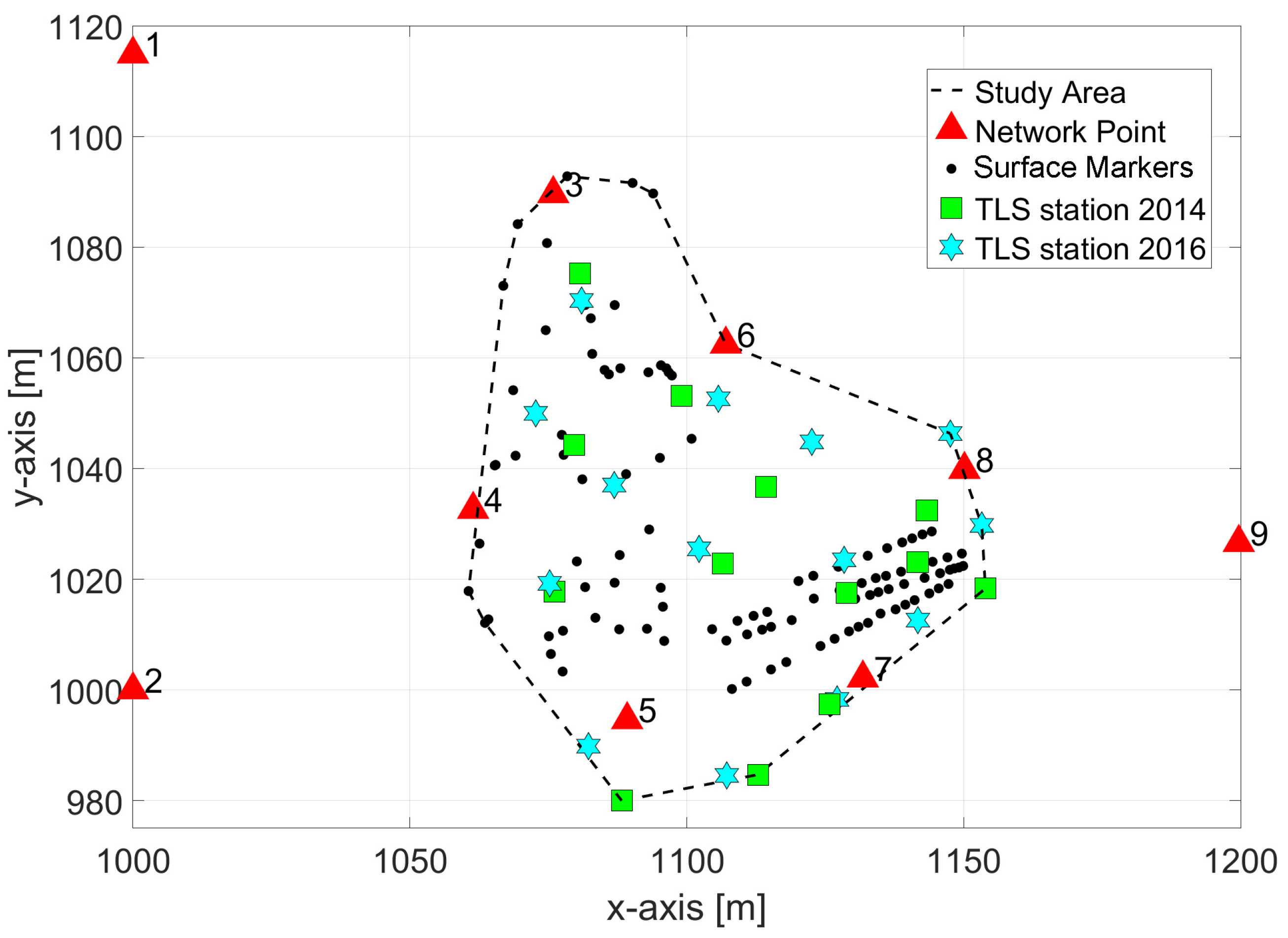
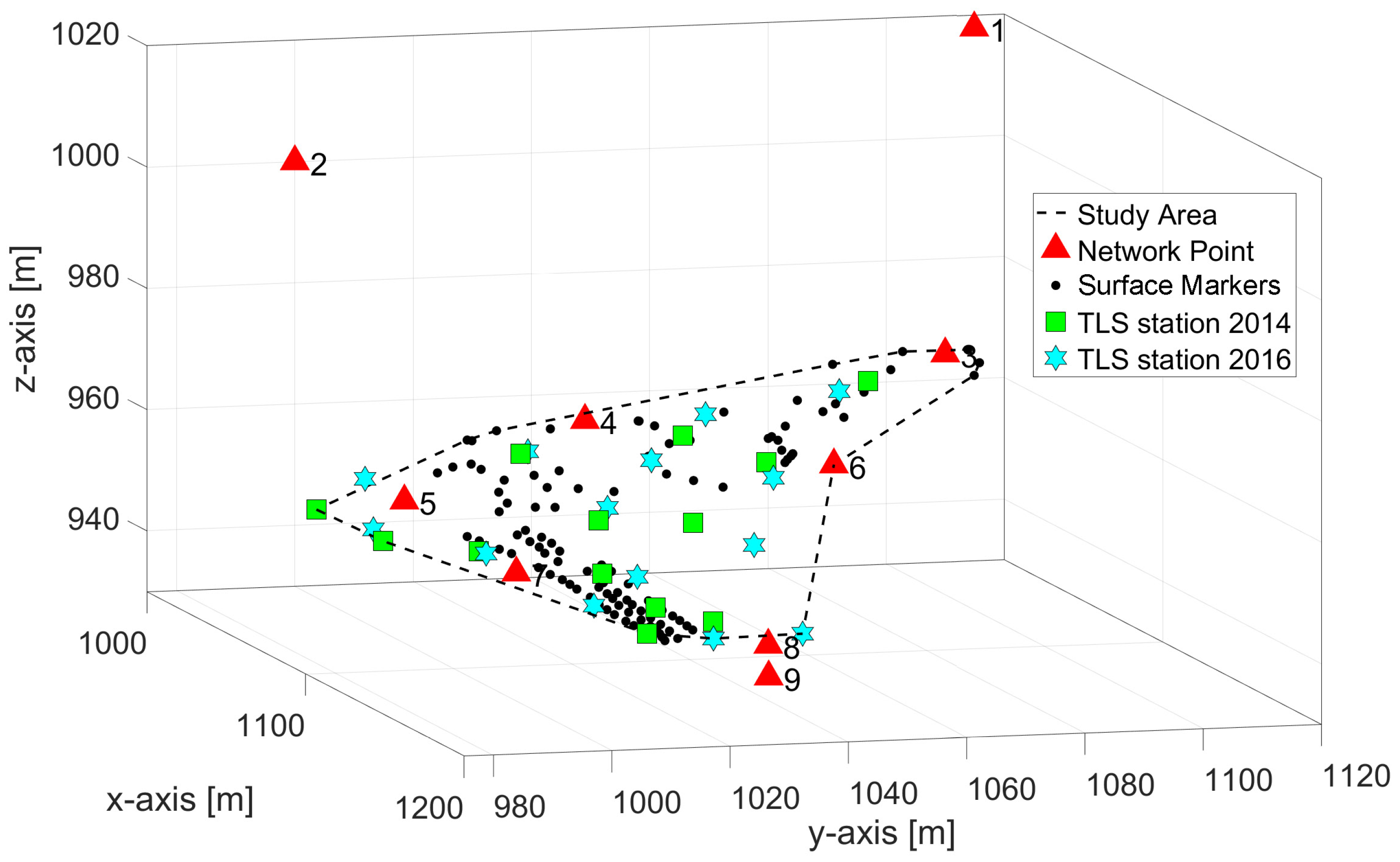
We analysed the soliflucion, i.e., the surface velocities and pattern of deformation of adjecent lobes, in the Austrian Alps (Figure 1). Section 3.1 presents the test area where the measurements were performed during the summer season of years 2014 and 2016. To determine the geometric changes between both years with sufficient accuracy, we established a common local coordinate system according to the usual geodetic practices [59]. This coordinate system was fixed to the Earth’s surface by mounting and measuring a set of permanently stabilized points, and therefore realizing the reference frame and/or geodetic datum. This step is called georeferencing (more in Section 3.2) and it ensures that the measurements of both epochs can be linked to the same coordinate system and analysed within it. It allows for a comparison of the measurements and reveals the deformation velocity and pattern with high accuracy. We conducted both point-based measurements using a total station (Section 3.3), as well as the area-based measurements using a terrestrial laser scanner (Section 3.4) for comparison and validation purposes. The measurements were analysed and discussed in detail in the following sections.

3.1. Study Area

The study area (Figure 1) is located in the central Hohe Tauern range of the Austrian Alps, about 5 km south of the Großglockner (3798 m NHN—Normalhöhennull; height above sea level), the highest peak in the Eastern Alps. Here, the crystalline rocks of the penninic Tauern Window border the strongly weathered micashists and phyllites of the Shober mountains that dominate the small Glatzbach creek area [60]. At the southern fringe of the catchment, a prominent assemblage of solifluction lobes of different scales attaining lengths of up to 50–80 m with riser heights of up to 0.5 m is located between 2600 and 2700 m NHN, oriented towards the eastern and northeastern directions [6,61].

This field site has been the subject of earlier studies. Previous studies in the Glatzbach area by Stingl et al. (2010) [61] showed that the regolith at this altitude frquently shows thicknesse larger than 0.5 m and is composed of weathering products of limestone- and quartz-rich phyllites. This fine-grained substrate favours the widespread development of solifluction lobes with seasonal movements primarily taking place during the thawing period in late spring and early summer. Between 1985 and 2008, surface velocities were measured continuously using repeated GNSS surveys of more than 100 markers. Results show highly variable mean velocities between 2 and 20 cm per year, with peak velocities of individual markers attaining as much as 100 cm per year [20,61]. Despite the very long time series of measurements at the site, a rigorous analysis of the pattern of surface deformation in high-resolution is still missing.

3.2. Georeferencing

To define the aforementioned geodetic datum (Section 3), two strategies could be followed: In the first one, the datum is defined by acquiring the measurements directly in a georeferenced coordinate system. Thus, the instrument is localized and oriented in a global coordinate system before or during the measurements. For example, a GNSS-antenna could be placed directly on top of a laser scanner or a total station, which allows for direct estimation of their position in one of the global coordinate systems, e.g., in World Geodetic System 1984 (WGS84), see, e.g., [62]. Alternatively, the instrument is georeferenced indirectly by measuring a set of stable points whose positions are previously defined in a global coordinate system. Hence, the local instrument’s coordinate system is transformed into a global one by exploiting the known correspondences between the coordinates in the instrument’s and the global system, for example, within the least-squares adjustment, see, e.g., [63].

While the direct georeferencing is more efficient, since no stable points have to be signalized and measured, it lacks dependence on the quality of the sensor observations used for georeferencing, e.g., GNSS observations [4]. Usually, this strategy leads to less accurate point positions and, most importantly, to point positions that might vary between two epochs or that cannot be estimated well enough. Since we seek to detect geomorphological processes with velocities in the order of a few centimetres a year, we used the more accurate indirect georeferencing strategy.

Hence, to realize the local coordinate system, we permanently mounted nine points, forming a geodetic network (depicted in Figure 2 in 2D, and in Figure 3 in 3D, and marked as “Network Points”). Three points (number 1, 2, 9) were permanently mounted on stable bedrock outcrops outside of solifluction features. For this, we used a drilling machine and marked the holes with surveying points. The origin of the local coordinate system is defined in point “2” with the values of 1000 for the x- and y-axis to avoid calculations with negative coordinates. The direction of the y-axis points towards the point “1”, while the x- and z-axis complement a right-handed coordinate system. Additionally, we placed further six points in the vicinity of the area potentially affected by solifluction. Two of them (number 6, 7) are again installed in the bedrock, while four of them (3, 4, 5, 8) are placed in unconsolidated material. The latter points are likely to shift between measurement epochs; however, they were deemed and attested as stable during each individual epoch. Hence, including them in the network adjustment improves the geometry and increases the quality of the underlying geodetic network. In other words, although the long-term stability of these points is questionable, they allow for a more accurate estimation of the relative positions of other stable points within each epochs. Finally, from all nine “Network Points”, only the ones that were confirmed to be stable between the epochs in the deformation analysis (see Section 4.1) were used for estimating the transformation parameters (georeferencing).

3.2.1. Data Acquisition

All Network Points were measured in both epochs based on the conventional measurements of geodetic networks [59] with the total station Leica TS30. Thus, all points were signalized with high precision prisms on surveying tribrachs and tripods. The total station was successively placed on each tripod to measure vertical angles, horizontal directions and slope distances to all other visible points. Leica TS30 is a high-end instrument with measurement accuracy in the sub-millimetre-to-millimetre level for the slope distance measurements (0.6 + 1 ppm) and 0.5 arc seconds for the angular measurements [64]. To additionally guarantee high accuracy and reliability, these measurements were performed repeatedly using strategies to eliminate potentially existing random and systematic errors in the whole measurement process. This procedure has been established in engineering geodesy for decades, see, e.g., [63], but has rarely been applied in a geomorphologic context.

Total stations, and also the terrestrial laser scanner used later, measure the slope distances electro-optically using the phase-shift or time-of-flight measurement principle. When measuring the distances based on an emitted laser beam, the refractive index that determines the speed of that laser beam in the atmosphere needs to be known [63]. This refractive index mostly depends on the air temperature and pressure, while the humidity is less important. If this refractive index is not known along the travelled path of the laser beam, the measured distance is biased with a scale-related systematic error, reducing the measurement accuracy. This leads to systematically too-long or too-short distance measurements:

• Changes in the air temperature of a 1 ${}^{\circ }$C increase or decrease, respectively, the distance by 1 mm/km (+1 ${}^{\circ }$C causes −1 mm/km);
• Changes in the air pressure of a 3 hPa increase or decrease, respectively, the distance by 1 mm/km (+3 hPa causes +1 mm/km).

Thus, we also frequently measured the air temperature and pressure at the instrument and target positions and corrected the measured distances accordingly.

3.2.2. Data Processing

We analysed the quality of all measurements and the derived coordinates of Network Points in both epochs based on a geodetic network adjustment. The approach outlined below equals a classical geodetic point-based deformation analysis described in many text books, e.g., [65]. The processing chain includes the following steps for each epoch:

• Analysing the observations from each station, eliminating outliers, reducing random and systematic errors following geodetic basics;
• Applying corrections to all measured distances accounting for changes in air temperature and air pressure based on the recorded values;
• Estimating the coordinates of the network points in a network adjustment based on the least-squares;
• Assessing the quality of the network: Analysing the estimated covariance matrices of the network points as well as the partial redundancies of each observation. While the first aspect concerns the accuracy of the network, the second one describes its reliability, i.e., its ability to detect outliers.

After these steps are performed for both epochs (2014 and 2016) separately, both sets of coordinates were tested for congruency to fix the datum identically for both epochs [65]. Therefore, the “two-epoch-comparison” is used to test whether each network point moved between epochs or its position remained stable. This statistical test is needed, since differences between the point coordinates could be caused by random measurement errors or an actual movement of the point. Without a statistical test, these possibilities could not be separated.

The points that remain stable between both epochs are used to fix the final geodetic datum, and they are commonly called “datum points”. Hence, only these datum points were used to finally georeference all local measurements, whose acquisition is described in Section 3.3 and Section 3.4.

3.3. Point-Based Measurements with Total Station

The most prominent solifluctional tongues and lobes have been signalized, with 20-cm-long PVC rods inserted halfway into the ground. These surface markers helped to map the spatial distribution and variability of solifluction rates at several discrete points, as shown in Figure 2 and Figure 3. In sum, in both epochs, we relied on 104 markers that were deployed in an earlier study [20].

We positioned the total station (Leica TS30) in the study area between network points 7 and 8. From this position, all surface markers were visible after signalizing each with a prism mounted on a plumb rod. All 104 markers were measured in both epochs in the local coordinate system, realized by the total station. Additionally, we measured Network Points for later georeferencing. Again, air temperature and pressure were recorded during these measurements.

We applied the necessary corrections to all distance measurements (see Section 3.2.2) and calculated 3D coordinates of each surface marker. After georeferencing these coordinates for each epoch separately, the difference vectors of all 104 markers between both epochs were calculated to represent the land-surface movements in the study area.

3.4. Area-Based Measurements with Terrestrial Laser Scanner

Contrary to the total station measurements of a finite number of signalized surface markers, a terrestrial laser scanner samples the whole surrounding area without the requirement of special reflectors positioned above known points. The measurement rate and the resulting point density and the amount of captured details are tremendously higher. For example, the commercial laser scanners commonly have a measurement rate of 1 million points per second, with a point spacing of only several millimetres or centimetres [43]. The data acquisition and processing are explained in the following text.

We scanned the whole study area with a laser scanner Leica ScanStation P20 from 13 stations in 2014 and 14 stations in 2016 (Figure 2 and Figure 3, green and blue markers). The position of each station was chosen considering that the solifluction lobes should be measured in detail and without any occlusions. The positions were selected similarly for both epochs, so that the eventual systematic errors due to changes in measurement configuration (distance and angle of incidence) and due to changes in the field of view (most of the instrumental errors are elevation-dependent) would be of minor importance when building the epoch-wise difference between point clouds. In other words, all eventual systematic errors would remain similar and cancel each other out to a large degree when building the differences. Additionally, this assured that similar details in the study area are captured with a similar resolution, which is important for the developed deformation monitoring workflow presented in Section 3.4.3.

All scans were acquired with a resolution of 3.2 mm at 10 m distance, leading to a point spacing in the complete test area of at least 20 mm and about 80 million points. Figure 4A,B depict a top-down and 3D view of the 16 square meters area of a point cloud, coloured according to the intensity of the reflected laser beam. It can be seen that the reflective properties of the scanned surface are quite inhomogeneous. This can be explained by the vegetation cover on a surface that is highly variable on a centimetre scale. Consequently, the measurement precision noticeably varies between points and pochs, as it is proportional to the intensity according to the intensity-based stochastic model presented in [66].

Analogue to the total station measurements, all necessary corrections were applied to the distance measurements. Afterwards, the point clouds of all stations were registered into a common local coordinate system using laser-scanning targets (black and white check-board planar targets) that were installed on tribrachs and tripods and distributed over the complete study area. The point cloud registration was achieved with high accuracy, where the standard deviation of target residuals was 1.3 mm per coordinate (2.2 mm in 3D). Next, the resulting point cloud of each epoch was georeferenced using the datum points that were also signalized with the laser-scanning targets. The georeferencing accuracy was comparable with the standard deviation of target residuals of 1.1 mm per coordinate (1.9 mm in 3D). Figure 4C depicts the resulting georeferenced point cloud in three dimensions.

To determine geometric changes, the point clouds of the entire study area from 2014 and 2016 are compared with each other, using several different methods. The data processing of these methods is described in the following subsections.

3.4.1. Data Processing: Point Cloud Comparison

For the point-cloud-based strategy (see Section 2), the M3C2 algorithm [46] is chosen as the best-established method, especially in earth sciences when dealing with irregular surfaces. It allows a for the robust comparison of two point clouds with increased sensitivity towards deformations in the direction of the local surface normals. This increased sensitivity is achieved by locally fitting small planar patches, which strongly reduces the measurement noise. For more information on point cloud comparisons in general, and the M3C2 algorithm in particular, see [57]. The result of the comparison is a so-called color-coded inspection map with a color representation corresponding to the signed distances between point clouds. This map is later used to draw conclusions about the movement of the lobes in Section 4.

3.4.2. Data Processing: Local ICP

Another representative method belonging to the same strategy (see Section 2) which is used in this study is the calculation of transformation parameters by ICP algorithm between the smaller local regions extracted from the complete point clouds. Here, large transformation parameters indicate a deformation within the corresponding regions. These regions can be defined and extracted automatically by dividing the complete measured object into cells of equal size, as was performed in [67] with the ICProx algorithm. Alternatively, the regions can be manually defined based on prior knowledge, which is potentially more meaningful for a particular study. Herein, we adopted the latter approach.

Our prior knowledge was based on the previously conducted M3C2 point-cloud comparison. Namely, regions that seemed to be deformed based on the M3C2 were further analysed by calculating the local transformation parameters between both epochs using the ICP. These regions represented the individual lobe tongues that were extracted from both georeferenced point clouds. Figure 5 presents one such example. Based on the estimated transformation parameters, a displacement vector can be calculated that describes the movement of the respective lobe tongue.

It is worth noting that both of the aforementioned approaches are primarily sensitive in the direction of the local surface normals. This can mean that a large portion of the deformations occurring along the land surface remains undetected. That was largely investigated in [9], which clearly indicated the advantages of the “point-based” point-cloud comparison strategies (see Section 2), where they proved that 3D vector fields can much more faithfully represent the deformations of landforms. However, the approach developed in the latter study cannot reach sufficient accuracy to detect the deformations of several centimeters, as was expected in the present study. Therefore, this was the motivation for developing a new “point-based” comparison strategy, which is presented in the following section.

3.4.3. Data Processing: Feature Detection and Tracking

As the most advanced method, we propose a new workflow which falls into the category of the point-based deformation-monitoring strategies with point clouds (see Section 2). The method generates a dense 3D vector field with the accuracy of each resulting vector ranging from millimetres to a few centimetres. This allows the analysis of the solifluction with increased spatial and temporal resolution, allowing for better understanding of the underlying processes.

This workflow is specifically developed for monitoring slowly moving landforms, which are typically observed in longer time intervals in comparison to the fast-moving natural objects and phenomena, such as landslides, glaciers or icebergs. Hence, it overcomes the deficiencies of the existing approaches:

• It does not require permanent mounting of a sensor and continuous monitoring from a single viewpoint [11,14,15];
• It is not limited to detecting displacements only in 2D [4,14,15];
• It can achieve sufficient accuracy of the 3D displacement vectors to faithfully capture the motion of slowly moving landforms, such as solifluction lobes, which cannot be guaranteed with the existing approaches [4,9,11,14,15].

The developed workflow relies on feature detection and matching, which is commonly used in image processing to detect distinctive points in an image and to match the corresponding points between similar images [68]. As the result is a 3D vector field describing the motion of the detected features between two epochs, we refer to the presented workflow as feature detection and tracking. To apply image-processing algorithms, the registered point cloud is rasterized in a corresponding image representation in two steps. First, it is transformed in a digital elevation model (DEM) with a millimeter-level resolution and with a projection plane spawning through the XY-plane of the local coordinate system. As laser scanners do not sample the surroundings in a regular Cartesian grid, an interpolation step was necessary to assign the height values for all empty pixels in the DEM. Additionally, if more than one measurement fell within one pixel, these measurements were simply averaged. Second, the resulting DEM is processed by the hillshading technique for creating relief maps [69], which indicates relative slopes and ridges rather than absolute heights. This step increases the amount of detail that can be identified and correctly matched between two measurement epochs.

Distinct points in the resulting hillshade images are detected using the minEigen algorithm [70], while the detected points are uniquely described regarding their local surrounding using the KAZE feature description algorithm [71]. The latter two algorithms were selected as they provided the largest number and the best distribution of matched points from several tested methods. The matching of the detected and described corresponding points results in numerous (more thousands) vectors representing the direction and magnitude of point movements between two measurement epochs.

The main problems of the feature detection and matching in image-processing are an inevitably large number of false matches and relatively poor localization precision of each individual feature. These problems are tackled by a filter tuning, an outlier elimination and an averaging step. The filter tuning aimed to select the minEigen and KAZE algorithm parameters that produced the minimal number of false matches and, in our study, it was optimized for the study area.

For the outlier elimination, a special strategy was developed that relies on the premise that all neighboring points move in similar direction and with a similar magnitude. Therefore, two histograms were created from all neighboring vectors connecting the matched points of two measurement epochs: one histogram with the vector magnitudes and one with their orientation. The histograms’ maxima indicate the general direction and magnitude of the lobe’s movement in a particular region. All vectors that were notably different regarding the subjectively defined threshold were deemed outliers, and therefore eliminated. In the final step, numerous unordered vectors are locally averaged (median) in a regular grid forming a 3D vector field. This step increases the precision of the estimated displacement vectors. The neighbourhood for histogram-based outlier determination is approximately three times larger than the one used for the final local averaging to increase the sample size and assure local congruency. The results of this workflow are presented in the following section, and its success with respect to the traditional point-wise and other point-cloud-based deformation-monitoring methods are discussed in detail in Section 5.

4. Results

In this section, we first evaluate the accuracy of the georeferencing (Section 4.1), then the point-based monitoring method (Section 4.2) and, finally, the three tested area-based monitoring methods (Section 4.3).

4.1. Georeferencing

After processing the total station measurements (outlier detection and all corrections), we estimated the point coordinates of the “Network Points” of both epochs (2014 and 2016) in the geodetic network adjustment (see Section 3.2). The coordinates of the points (epoch 2014) and their differences between the epochs are shown in

Table 1. Results of the network adjustment: Coordinates of Network Points in the year 2014, its 3D accuracy $\sigma$ (estimates based on the coordinates covariance matrix from the network adjustment), the movements between 2014 and 2016 along each axis (${\Delta }_x$, ${\Delta }_y$, ${\Delta }_z$), in 2D (${\Delta }_{2D}$), in 3D (${\Delta }_{3D}$) and the labeling of stability.

No.	x [m]	y [m]	z [m]	${\mathit{\sigma }}_{\mathit{xy}}$ [mm]	${\mathit{\sigma }}_{\mathit{z}}$ [mm]	${\Delta }_{\mathit{xy}}$ [mm]	${\Delta }_{\mathit{z}}$ [mm]	Stable
1	999.9919	1114.8805	1017.8782	<0.2	<0.8	1.7	−0.9	yes
2	999.9942	999.9980	1000.0019	<0.2	<0.8	1.0	−0.5	yes
3	1075.8894	1089.6349	975.3597	<0.2	<0.8	70.3	−20.9	no
4	1061.4230	1032.5943	964.5047	<0.2	<0.8	26.1	0.0	no
5	1089.2357	994.6102	956.3786	<0.2	<0.8	61.0	−8.2	no
6	1107.0519	1062.4591	962.2790	<0.2	<0.8	0.1	−3.7	yes ($xy$)
7	1131.7983	1002.1349	950.0082	<0.2	<0.8	0.2	1.3	yes
8	1150.1347	1039.8193	939.2219	<0.2	<0.8	4.6	2.4	no
9	1199.6758	1026.6174	941.1861	<0.2	<0.8	0.9	0.2	yes

.

According to a geodetic deformation analysis [65], the coordinate differences between both epochs, here expressed by the vector $\Delta$, are statistically evaluated considering their uncertainty, here expressed by $\sigma$. Since the uncertainty is less than 1.0 mm for each point (based on the covariance matrix of the estimated coordinates in the network adjustment, see Section 3.2.2), even displacements of several millimetres can be detected.

The deformation analysis of the points affirmed the points 1, 2, 6, 7, and 9 as stable points. They did not move between the two epochs within the uncertainty range denoted in Table 1 and were therefore used to fix the geodetic datum, i.e., they were used for georeferencing. The statistical deformation test, according to [68], is based on a probability level of 99.7%.

Contrary, the points 3, 4, 5, and 8 are identified as unstable within the deformation analysis. These points showed significant movements between 5 and 74 mm and are shown in Figure 6 as red vectors. They give a first indication of the magnitude of the movement in the unstable region of investigation.

4.2. Point-Based Measurements: Comparison of Surface Markers Coordinates

As described in Section 3.3, after georeferencing, the point coordinates of all surface markers (Figure 2 and Figure 3) in both measurement epochs were calculated and then compared with each other. The differences are shown as green vectors in Figure 6. It can be seen that the points moved differently between 2014 and 2016. At some locations, the movements reached up to 220 mm. The movements of neighbouring surface markers point to similar directions and have similar orders of magnitude. The direction of movement also matches the expected flow direction of the lobes, as they point to the direction of the lower areas. This confirms that the accuracy of this established pointwise geodetic approach was sufficient for this task of monitoring the slowly moving solifluction lobes with a given temporal resolution.

From the different vector lengths within the study area, it can be concluded that there are more active and less active regions. However, a clear identification of individual lobes is not possible, because of the wide gaps between the sparse number of surface markers where no motion information is obtained. Hence, this strongly limits the spatial resolution. This gap is filled by the analysis of the area-based measurements with TLS and with the newly developed point-based monitoring workflow.

4.3. Area-Based Measurements: Point Cloud Comparison

Figure 7 depicts the color-coded inspection map, which is a result of the M3C2 algorithm for the point-cloud comparison (see Section 3.4). The false-color map represents the land surface movements, where the green color corresponds to no movement between the epochs, while the detected movements are presented with a gradual color change towards blue and red (depending on the magnitude and direction/sign).

In contrast with the point-wise analysis, the information of the entire study area is available, with high spatial resolution. As can be seen in the figure, the majority of the area is green, indicating that this method presumes that the point-cloud differences, i.e., movements, were only a few millimetres in most regions. In contrary, small red and blue regions represent locations where the point clouds differed by up to 70 mm.

From the existing literature, see, e.g., [57], it is known that this method is only sensitive for the detection point-cloud differences in the direction of the local surface normals. Hence, the so-called “out-of-plane” deformations, i.e., deformations perpendicular to the local surface, can be identified with high accuracy. However, the so-called “in-plane” deformations, i.e., along the measured surface, cannot be detected at all. This can explain the appearance of Figure 7: At the fairly planar parts of the surface, the M3C2 algorithm detects no land-surface movements. However, in the neighbourhood of the lobe’s heads, larger differences occur. Since the lobe moved from left to right, in a downhill direction, in Figure 7, the point cloud comparison results in positive differences downhill from the lobe’s head, and in negative differences at the position where the lobe’s head was in the first epoch. Hence, characteristics patterns of deformations appear, which are positive differences directly followed by negative ones. Based on this definition, 10 prominent lobes can be identified in Figure 7, and they are marked with black circles.

To conclude this analysis, there are three important observations:

• This method does not rely on the pre-determined positions of the previously fixed markers. Hence, it can detect discrete movements over the whole study area, avoiding the pitfall of having large gaps between the measurements. This means it can reveal movement, even in regions where it was not a priori expected;
• However, the detected movements are still discrete, appearing only in locations where the movement was approximately perpendicular to the land surface. Therefore, although this approach has obvious advantages in comparison to the point-wise measurement method with a total station, it still lacks a high spatial resolution to faithfully represent the lobes’ movement;
• Finally, this method provides the magnitudes of the movement only in one direction (1D), perpendicular to the surface. Hence, it is not suitable for deriving 3D vector fields. Hence, it cannot reveal the full magnitude and the exact direction of the surface movement.

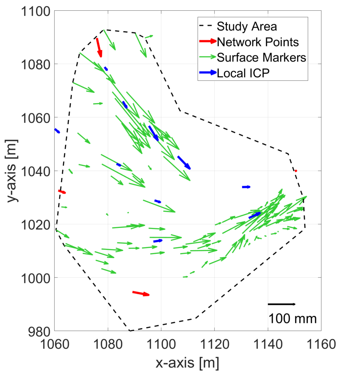
4.4. Area-Based Measurements: Local ICP

Estimating the local surface movements as a set of transformation parameters acquired by locally running an ICP algorithm (see Section 3.4) alleviates some of the pitfalls of the previous method. The results of this method are 3D vectors (instead of 1D distances from M3C2 algorithm) corresponding to the transformation parameters of the matching point-cloud regions between two epochs. Hence, the land surface movement can be represented with higher fidelity.

Herein, we selected the point-cloud regions corresponding to those lobes’ heads, which were identified by the M3C2 algorithm in the previous step (black circles in Figure 7A). The vectors of the local transformations are depicted in Figure 6 in a blue color, and they are quantified in

Table 2. Displacements for lobes’ heads based on the local ICP.

No.	x [m]	y [m]	z [m]	${\Delta }_{\mathit{xy}}$ [mm]	${\Delta }_{\mathit{z}}$ [mm]	$\mathit{\sigma }$ [mm]
1	1097	1013	954	30.3	10.2	≈2
2	1095	1056	962	62.5	12.7	≈2
3	1106	1045	957	64.2	12.3	≈2
4	1085	1066	966	27.1	11.6	≈2
5	1078	1078	971	13.5	16.1	≈2
6	1060	1055	968	20.7	5.9	≈2
7	1097	1028	955	21.5	7.2	≈2
8	1132	1022	945	45.2	10.7	≈2
9	1130	1033	945	27.2	4.1	≈2
10	1083	1042	961	15.0	14.6	≈2

. Comparing these results with the previous ones reveals three important observations:

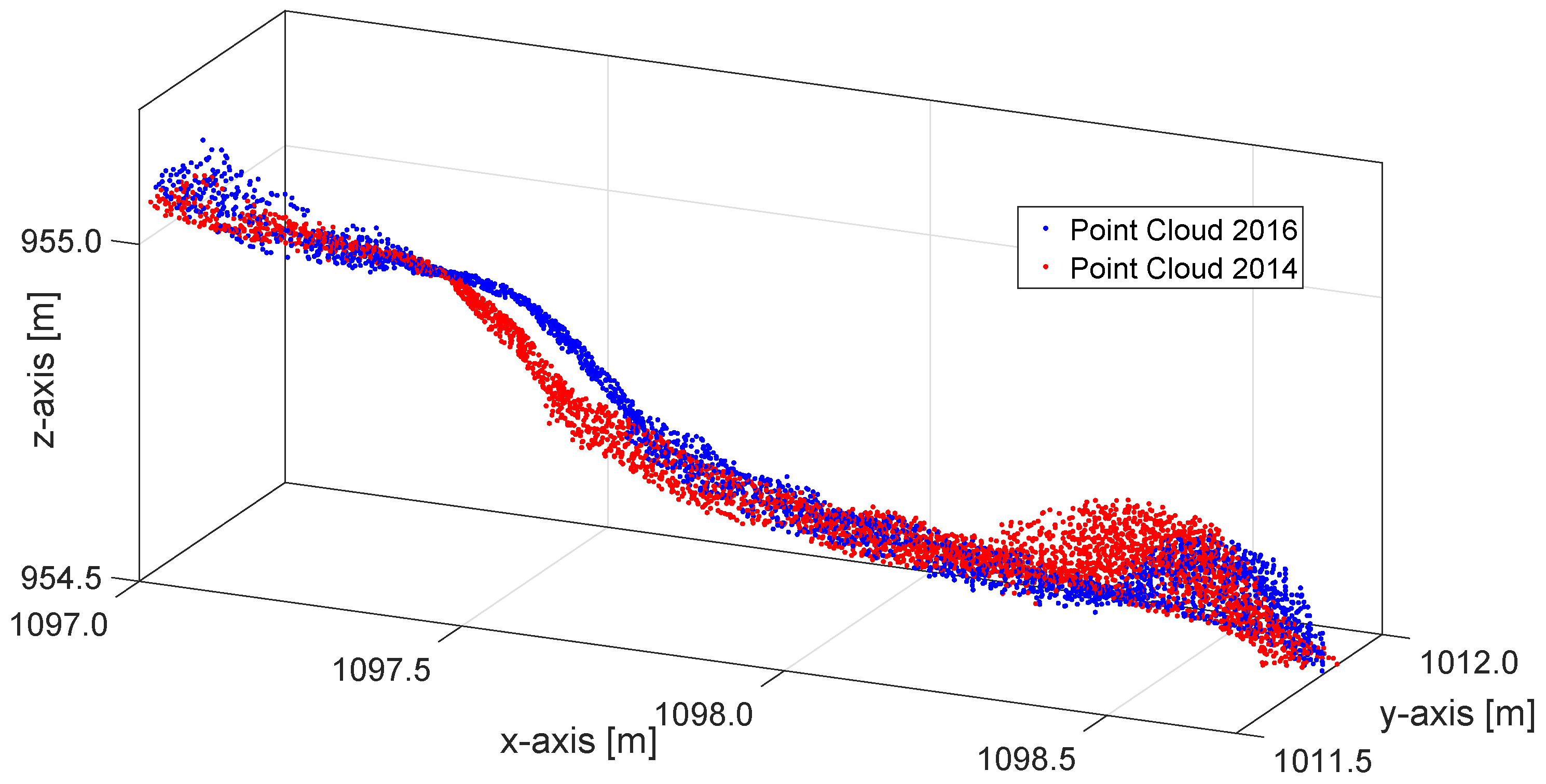
• First, we can observe the maximal vector lengths of about 65 mm, which are considerably smaller in comparison to the ones from the point-wise measurements (approximately 220 mm). Furthermore, if we compare the blue and green vectors in Figure 6, it is noticeable that the ICP-based movement magnitudes are actually smaller in every instance than the ones of the surface markers. Hence, like the M3C2 algorithm, this method is also not always capable of revealing the full magnitude of the movement. This is due to the fact that the ICP algorithm, despite being able to generate 3D vectors instead of 1D distances, is still only sensitive to movements in the direction of the local surface normals (1D);
• Second, we can observe that this method successfully and accurately detected the directions of the movements, which completely correspond to the directions estimated by measuring the surface markers. Hence, the advantage of this method in comparison to the M3C2 is the possibility of correctly parametrizing the direction of the surface motion;
• However, third, this is only possible if the distribution of surface normals in some smaller regions is relatively high, such is in the case of the lobes’ heads. For example, if the region contains some larger structural elements, such as rocks, the 3D motion of the surface can be reconstructed. Nevertheless, if the region is fairly planar, the complete motion can be overlooked. Thus, the true motion of the land surface can be estimated only in discrete locations and not over the whole surface. This, again, results in the limitation of the spatial resolution.

In most real-world cases in earth sciences, the situation will be somewhere in the middle of a volumetric or well-distributed surface in all three directions and a completely planar land surface. Hence, it will be possible to estimate the motion direction in many discrete instances within the study areas. However, the magnitudes of the motion will potentially be underestimated, as can be seen in Figure 6.

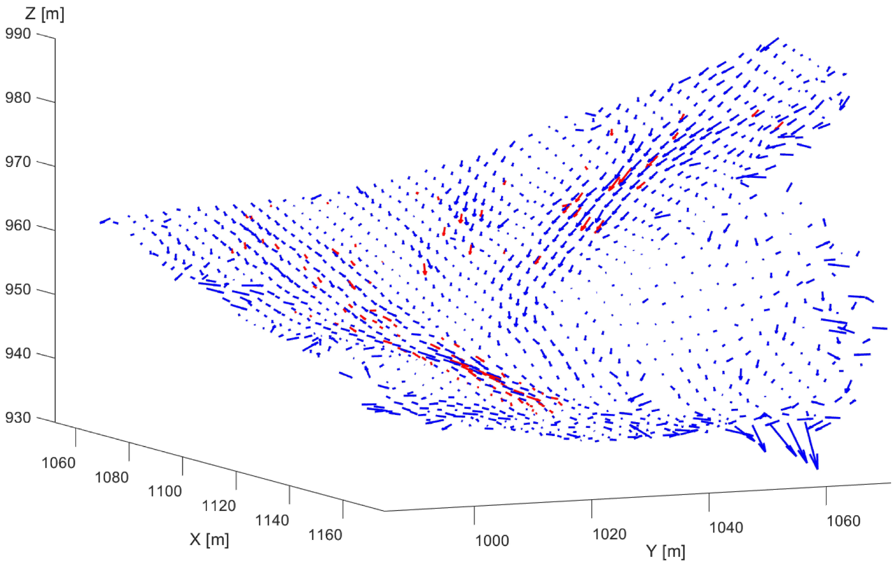
4.5. Area-Based Measurements: Feature Detection and Tracking

As mentioned, the result of the feature-tracking algorithm described in Section 3.4 is a 3D vector field representing the landform movements in the whole study area with high spatial resolution and accuracy. The results are presented in 2D in Figure 8 with blue arrows, while the red arrows indicate the surface markers already shown in Figure 6. Additionally, for a better interpretation, the same results are presented in 3D in Figure 9. Both figures imply a strong coherence between feature-tracking and surface markers, in the displacements’ directions as well as in their magnitudes.

To quantify this coherence, we first estimated the nearest neighbouring vectors from both datasets using the naive method based on the Euclidean distance. Then, we computed the differences in the corresponding vectors in the direction of each coordinate, as well as the differences in 2D and 3D magnitudes (vector norms). Based on these differences, we computed the standard deviation and the median absolute deviation (MAD). The latter value is a preferred measure for the data distribution in the presence of eventual outliers, which are quite common for the feature-matching algorithms, such as the one implemented in the workflow described in Section 3.4.

The results of the comparison showed that the standard deviation of the 2D and 3D vector magnitude differences was 2.5 cm, while MAD was only 1.4 cm when all 104 surface markers were considered. There is no notable difference if the magnitudes of 2D or 3D vectors are compared, because the Z-components of all vectors are comparably small (in the range of several millimetres).

Expecting smaller values than these would have been unreasonable. Namely, Ridefelt et al. (2011) [72], in their investigation, showed that the methodological error of total station measurements of the surface markers is in the level of 1 cm, with the additional observer errors in the range of 0–1.5 cm. When we add the uncertainty of matching the corresponding vectors with potential false matches (outliers), as well as the uncertainty of the laser scanner measurements, we land within the expected value range that was achieved in this analysis.

We also investigated the eventual existence of the systematic biases between two deformation monitoring strategies. There, we found out that the magnitudes of the 3D displacement vectors generated with the proposed feature-detection and -tracking method were, on average, (median) 1.0 cm larger than ones computed from surface markers. This value is within the same range as the expected measurement uncertainty presented above. However, in our future work, we will investigate the origin of this phenomenon, as eliminating it would further improve the results of the implemented workflow.

Thus, it can be concluded that there are no notable differences between the established reference point-wise measurements with total station and the developed workflow. This means that the developed workflow provides the accuracy of single 3D vectors in the order of at least a few centimetres, with notably higher spatial resolution than the reference approach. Unfortunately, the exact accuracy would be hard to assess, as realizing the reference measurements that are at least 3 to 5 times more accurate in such measurement setup would be unfeasible, if not impossible.

However, there is another, rather qualitative, sign that the accuracy of the derived 3D vectors is potentially even higher. This depicts the down-slope material flow of the whole assemblage of small-scale solifluction lobes, as well as the locations of the stable regions within the study area.

One of the main noticeable limitations of this method is accurate detection of the surface movement at the edges of the measured surface. This is prominent in Figure 8 and Figure 9 in the high random scatter of the vector directions and magnitudes at the point-cloud limits. Hence, it is advised to additionally measure the area exceeding the boundaries of the eventual region of interest.

To conclude, the developed workflow achieved an accuracy that is directly comparable to the established point-wise approach, allowing for an equally high temporal resolution when monitoring the solifluction lobes. However, in addition, it realized a much higher spatial resolution (1220 vs. 104 vectors) allowing for the generation of a dense and descriptive 3D vector field. In other words, it shows that both point-wise- and area-based approaches are capable of depicting the spatial variability of solifluction-related surface deformation, with faster displacement focused towards the centre of individual lobes. Nonetheless, we stress here that a higher spatial resolution of the derived area-based approach can resolve this variability in much greater detail. Further discussion of the developed workflow, as well as comparison to the other applied approaches and to the state-of-the-art monitoring methods, are provided in the following section.

5. Discussion

Considering all the results together, several main conclusions can be summarized and discussed:

• The point-wise measurements with total station and surface markers allow for the determination of movements at discrete points on the lobes’ surface. The disadvantage of this standard geomorphological method is that the spatial resolution of the measurements is very limited. However, measurement accuracy is relatively high, allowing for the detection of even small-scale land-surface movements;
• The comparison of TLS point clouds based on an M3C2 algorithm allows for the detection of changes in the geometry and volume at lobes’ heads. Unlike the previous method, it has increased spatial resolution in a sense that it is not restricted to a pre-determined set of marker locations. However, it is still limited to a few discrete locations, as detection is only possible where the surface structure allows for change detection. In such locations, it is possible to identify where the volume increases and decreases. However, it is not possible to estimate the exact magnitude and direction of the lobes’ movements [57];
• The transformation parameters determined locally with the ICP algorithm increase the amount of extracted information from point clouds by allowing for the estimation of correct directions and biased magnitudes. The magnitudes are systematically underestimated, as the ICP is sensitive to change detection only in the direction perpendicular to the observed surface. This also means that this method is limited to monitoring discrete locations where the land surface normals are parallel with the solifluction direction (at lobes’ heads);
• Finally, the developed feature detection and tracking workflow can be used to derive surface movements with similar measurement accuracy and fidelity to the established point-wise method, without being restricted to pre-determined marker locations, and produces a 3D vector field with high spatial resolution covering the whole study area.

This analysis demonstrates the clear advantages and disadvantages of the available point-wise- and point-cloud-based methods for monitoring the displacement of natural surfaces. It is evident that the methods focusing on the automatic detection and matching of salient points in the surroundings, and, consequently, the generation of 3D vector fields, are the most promising ones in terms of monitoring the behaviour of various landforms. However, the other presented methods can be used to draw some relevant information as well.

In the future, the developed workflow should be compared with similar approaches that are capable of monitoring the natural objects with high spatial resolution, i.e., capable of generating dense 3D vector fields. For example, the UAV imagery-based approach relying on optical-flow, developed in [4], has some indications that a similar level of accuracy could be possible with a more cost-efficient measurement approach. Unfortunately, a fair comparison at this point was not possible, as the authors provided no quantitative measures for the accuracy of the derived displacement vectors. Additionally, they only implied that extending their solution to 3D is a possibility, where it is uncertain how accurately the height component can be estimated based on the point cloud derived by the photogrammetric reconstruction. Moreover, it would be interesting to see, on the same dataset, acquired with a terrestrial laser scanner, how competitive the method based on deep learning is, presented in Gojcic et al. 2020. In the latter article, the method reached some decimetre-level accuracy; however, the dataset was significantly different (landslide monitoring with airborne LiDAR).

Furthermore, it would be interesting to increase the measurement frequency and see to what extent this methodology could improve the temporal resolution when monitoring the slowly moving landforms. A higher measurement frequency with multiple epochs of the single objects could potentially provide new insights regarding the measurement accuracy. First, it would be possible to calculate some mean trajectory for multiple small regions, where the difference in each epoch could be related to the measurement errors. Secondly, it would potentially provide insight into the accuracy of estimating the solifluction velocities with high spatial and temporal resolution.

Finally, the generated results highlight the potential of high-resolution and high-accuracy monitoring of geomorphic processes in mountain areas. Though surface displacement rates from previous work at the same field site exceed our measurements, these studies also emphasize the large inter-annual variability of velocities [20,61]. We cannot rule out the possibility that the differential displacement rates obtained by our study and previous work are associated with measurement inaccuracies. However, we take the very good agreement between our independent point-based and area-based estimates as an indication that environmental factors, such as the length of the seasonal ground-thawing period, the duration of the seasonal snow cover and temperature variability, govern the inter-annual shifts in displacement magnitudes, see, e.g., [73]. Bearing this in mind, the very high accuracy achieved in our study allows for the intra-annual monitoring of solifluction, further contributing to a better understanding of how environmental conditions determine inter- and intra-annual surface velocity changes. In future, the developed approach should be further exploited by conducting higher frequency measurements in multiple epochs.

6. Conclusions and Outlook

In this study, we developed a new workflow to monitor slowly moving landforms based on terrestrial laser-scanner point clouds. The approach was tested based on a concrete case of the prominent assemblage of solifluction lobes in Hohe Tauern range of the Austrian Alps, and it was compared with established point-wise measurements of signalized markers with a total station, as well as point-cloud-based deformation-monitoring approaches.

The attested accuracy of the workflow’s results, in the order of a few centimeters (median absolute deviation to total station measurements of 1.4 cm), allows for the detection of small-scale displacements. Hence, this allows for the higher temporal resolution of monitoring the slowly moving solifluction lobes. Additionally, generating a dense 3D vector field assures high spatial resolution (a field of 1220 vectors vs. 104 markers measured with total station), which is necessary for better understanding of the solifluction processes.

The workflow primarily relies on the image-based processing techniques of feature detection/description and tracking (MinEigen and KAZE on a hillshade representation of a point cloud). Unlike the most similar approaches in the earth and ecological sciences, this does not require the permanent set-up of an instrument and continuous observations from a single viewpoint. Hence, it is better suited for monitoring slowly moving landforms, such as solifluction lobes.

In future, whether this workflow can be successfully applied to the point clouds derived by UAV platforms should be investigated, which would increase the overall efficiency of the approach. Additionally, it would be interesting to compare how this workflow measures up with the promising state-of-the-art techniques from Gojcic et al. (2020) [9] and Klingbeil et al. (2019) [4] on a common dataset. Finally, the increased measurement frequency should be used to both test the limitations of the workflow considering the temporal resolution, and to leverage its advantages and learn more about the solifluction processes. An interesting possibility would be to test the analysis approaches from the research area of fluid dynamics on the generated 3D vector field.

References

1. Matsuoka, N. Solifluction rates, processes and landforms: A global review. Earth-Sci. Rev. 2001, 55, 107–134. [Google Scholar] [CrossRef]
2. Ballantyne, C.K. Periglacial Geomorphology; John Wiley & Sons: Hoboken, NJ, USA, 2018. [Google Scholar]
3. Eitel, J.U.; Höfle, B.; Vierling, L.A.; Abellán, A.; Asner, G.P.; Deems, J.S.; Glennie, C.L.; Joerg, P.C.; LeWinter, A.L.; Magney, T.S.; et al. Beyond 3-D: The new spectrum of lidar applications for earth and ecological sciences. Remote Sens. Environ. 2016, 186, 372–392. [Google Scholar] [CrossRef] [Green Version]
4. Klingbeil, L.; Heinz, E.; Wieland, M.; Eichel, J.; Laebe, T.; Kuhlmann, H. On the UAV based Analysis of Slow Geomorphological Processes: A Case Study at a Solifluction Lobe in the Turtmann Valley. In Proceedings of the 4th Joint International Symposium on Deformation Monitoring (JISDM 2019), Athens, Greece, 15–17 May 2019; pp. 15–17. [Google Scholar]
5. Eichel, J.; Draebing, D.; Kattenborn, T.; Senn, J.A.; Klingbeil, L.; Wieland, M.; Heinz, E. Unmanned aerial vehicle-based mapping of turf-banked solifluction lobe movement and its relation to material, geomorphometric, thermal and vegetation properties. Permafr. Periglac. Process. 2020, 31, 97–109. [Google Scholar] [CrossRef]
6. Jaesche, P.; Veit, H.; Huwe, B. Snow cover and soil moisture controls on solifluction in an area of seasonal frost, eastern Alps. Permafr. Periglac. Process. 2003, 14, 399–410. [Google Scholar] [CrossRef]
7. Matsuoka, N. Solifluction and mudflow on a limestone periglacial slope in the Swiss Alps: 14 years of monitoring. Permafr. Periglac. Process. 2010, 21, 219–240. [Google Scholar] [CrossRef]
8. Fey, C.; Rutzinger, M.; Wichmann, V.; Prager, C.; Bremer, M.; Zangerl, C. Deriving 3D displacement vectors from multi-temporal airborne laser scanning data for landslide activity analyses. GIscience Remote Sens. 2015, 52, 437–461. [Google Scholar] [CrossRef]
9. Gojcic, Z.; Zhou, C.; Wieser, A. F2S3: Robustified determination of 3D displacement vector fields using deep learning. J. Appl. Geod. 2020, 14, 177–189. [Google Scholar] [CrossRef]
10. Wellmann, F.; Caumon, G. 3-D Structural geological models: Concepts, methods, and uncertainties. In Advances in Geophysics; Elsevier: Amsterdam, The Netherlands, 2018; Volume 59, pp. 1–121. [Google Scholar]
11. Dematteis, N.; Giordan, D.; Zucca, F.; Luzi, G.; Allasia, P. 4D surface kinematics monitoring through terrestrial radar interferometry and image cross-correlation coupling. ISPRS J. Photogramm. Remote Sens. 2018, 142, 38–50. [Google Scholar] [CrossRef]
12. Schrott, L.; Otto, J.C.; Götz, J.; Geilhausen, M.; Otto, J.C. Fundamental classic and modern field techniques in Geomorphology—An overview. Treatise Geomorphol. 2013. [Google Scholar] [CrossRef]
13. Eichel, J.; Corenblit, D.; Dikau, R. Conditions for feedbacks between geomorphic and vegetation dynamics on lateral moraine slopes: A biogeomorphic feedback window. Earth Surf. Process. Landforms 2016, 41, 406–419. [Google Scholar] [CrossRef]
14. Schwalbe, E.; Maas, H.G. The determination of high-resolution spatio-temporal glacier motion fields from time-lapse sequences. Earth Surf. Dyn. 2017, 5, 861–879. [Google Scholar] [CrossRef] [Green Version]
15. Kienholz, C.; Amundson, J.M.; Motyka, R.J.; Jackson, R.H.; Mickett, J.B.; Sutherland, D.A.; Nash, J.D.; Winters, D.S.; Dryer, W.P.; Truffer, M. Tracking icebergs with time-lapse photography and sparse optical flow, LeConte Bay, Alaska, 2016–2017. J. Glaciol. 2019, 65, 195–211. [Google Scholar] [CrossRef] [Green Version]
16. Lewkowicz, A.G. A solifluction meter for permafrost sites. Permafr. Periglac. Process. 1992, 3, 11–18. [Google Scholar] [CrossRef]
17. Matsuoka, N. Continuous recording of frost heave and creep on a Japanese alpine slope. Arct. Alp. Res. 1994, 26, 245–254. [Google Scholar] [CrossRef]
18. Jaesche, P.; Veit, H.; Stingl, H.; Huwe, B. Influence of water and heat dynamics on solifluction movements in a periglacial environment in the Eastern Alps (Austria). In Proceedings of the International Symposium Physics, Chemistry and Ecology of Seasonally Frozen Soils, Fairbanks, AK, USA, 10–12 June 1997. [Google Scholar]
19. Yamada, S.; Matsumoto, H.; Hirakawa, K. Seasonal variation in creep and temperature in a solifluction lobe: continuous monitoring in the Daisetsu Mountains, northern Japan. Permafr. Periglac. Process. 2000, 11, 125–135. [Google Scholar] [CrossRef]
20. Veit, H.; Stingl, H.; Emmerich, K.H.; John, B. Zeitliche und räumliche Variabilität solifluidaler Prozesse und ihre Ursachen-Eine Zwischenbilanz nach acht Jahren Solifluktionsmessungen (1985–1993) an der Meßstation. Z. FÜR Geomorphol. Suppl. Vol. 1995, 107–122. [Google Scholar] [CrossRef]
21. Sailer, R.; Bollmann, E.; Hoinkes, S.; Rieg, L.; Sproß, M.; Stötter, J. Quantification of geomorphodynamics in glaciated and recently deglaciated terrain based on airborne laser scanning data. Geogr. Ann. Ser. A Phys. Geogr. 2012, 94, 17–32. [Google Scholar] [CrossRef]
22. Kociuba, W. Assessment of sediment sources throughout the proglacial area of a small Arctic catchment based on high-resolution digital elevation models. Geomorphology 2017, 287, 73–89. [Google Scholar] [CrossRef]
23. Arenson, L.U.; Kääb, A.; O’Sullivan, A. Detection and analysis of ground deformation in permafrost environments. Permafr. Periglac. Process. 2016, 27, 339–351. [Google Scholar] [CrossRef]
24. Crawford, A.J.; Mueller, D.; Joyal, G. Surveying drifting icebergs and ice islands: deterioration detection and mass estimation with aerial photogrammetry and laser scanning. Remote Sens. 2018, 10, 575. [Google Scholar] [CrossRef] [Green Version]
25. Scaioni, M.; Roncella, R.; Alba, M.I. Change detection and deformation analysis in point clouds. Photogramm. Eng. Remote Sens. 2013, 79, 441–455. [Google Scholar] [CrossRef]
26. Kromer, R.A.; Abellán, A.; Hutchinson, D.J.; Lato, M.; Chanut, M.A.; Dubois, L.; Jaboyedoff, M. Automated terrestrial laser scanning with near-real-time change detection—Monitoring of the Séchilienne landslide. Earth Surf. Dyn. 2017, 5, 293–310. [Google Scholar] [CrossRef] [Green Version]
27. Kayen, R.; Pack, R.T.; Bay, J.; Sugimoto, S.; Tanaka, H. Terrestrial-LIDAR visualization of surface and structural deformations of the 2004 Niigata Ken Chuetsu, Japan, earthquake. Earthq. Spectra 2006, 22, 147–162. [Google Scholar] [CrossRef]
28. Wilkinson, M.; McCaffrey, K.; Roberts, G.; Cowie, P.; Phillips, R.; Michetti, A.M.; Vittori, E.; Guerrieri, L.; Blumetti, A.; Bubeck, A.; et al. Partitioned postseismic deformation associated with the 2009 Mw 6.3 L’Aquila earthquake surface rupture measured using a terrestrial laser scanner. Geophys. Res. Lett. 2010, 37. [Google Scholar] [CrossRef] [Green Version]
29. Kayer, R.; Stewart, J.P.; Collins, B.D. Recent advances in terrestrial LIDAR applications in geotechnical earthquake engineering. In Proceedings of the 5th International Conference on Recent Advances in Geotechnical Earthquake Engineering and Soil Dynamics, San Diego, CA, USA, 24–29 May 2010. [Google Scholar]
30. Pesci, A.; Teza, G.; Casula, G.; Loddo, F.; De Martino, P.; Dolce, M.; Obrizzo, F.; Pingue, F. Multitemporal laser scanner-based observation of the Mt. Vesuvius crater: Characterization of overall geometry and recognition of landslide events. ISPRS J. Photogramm. Remote Sens. 2011, 66, 327–336. [Google Scholar] [CrossRef]
31. Gumilar, I.; Abidin, H.Z.; Putra, A.D.; Haerani, N. 3D modelling of Mt. Talaga Bodas Crater (Indonesia) by using terrestrial laser scanner for volcano hazard mitigation. AIP Conf. Proc. 2015, 1658, 050008. [Google Scholar]
32. Slatcher, N.; James, M.R.; Calvari, S.; Ganci, G.; Browning, J. Quantifying effusion rates at active volcanoes through integrated time-lapse laser scanning and photography. Remote Sens. 2015, 7, 14967–14987. [Google Scholar] [CrossRef] [Green Version]
33. Telling, J.; Lyda, A.; Hartzell, P.; Glennie, C. Review of Earth science research using terrestrial laser scanning. Earth-Sci. Rev. 2017, 169, 35–68. [Google Scholar] [CrossRef] [Green Version]
34. Höfle, B.; Griesbaum, L.; Forbriger, M. GIS-Based detection of gullies in terrestrial LiDAR data of the Cerro Llamoca Peatland (Peru). Remote Sens. 2013, 5, 5851–5870. [Google Scholar] [CrossRef] [Green Version]
35. Kociuba, W.; Kubisz, W.; Zagórski, P. Use of terrestrial laser scanning (TLS) for monitoring and modelling of geomorphic processes and phenomena at a small and medium spatial scale in Polar environment (Scott River—Spitsbergen). Geomorphology 2014, 212, 84–96. [Google Scholar] [CrossRef]
36. Vericat, D.; Smith, M.; Brasington, J. Patterns of topographic change in sub-humid badlands determined by high resolution multi-temporal topographic surveys. Catena 2014, 120, 164–176. [Google Scholar] [CrossRef]
37. Williams, J.G.; Rosser, N.J.; Hardy, R.J.; Brain, M.J.; Afana, A.A. Optimising 4-D surface change detection: an approach for capturing rockfall magnitude–frequency. Earth Surf. Dyn. 2018, 6, 101–119. [Google Scholar] [CrossRef] [Green Version]
38. Anders, K.; Winiwarter, L.; Lindenbergh, R.; Williams, J.G.; Vos, S.E.; Höfle, B. 4D objects-by-change: Spatiotemporal segmentation of geomorphic surface change from LiDAR time series. ISPRS J. Photogramm. Remote Sens. 2020, 159, 352–363. [Google Scholar] [CrossRef]
39. Ulrich, V.; Williams, J.G.; Zahs, V.; Anders, K.; Hecht, S.; Höfle, B. Measurement of rock glacier surface change over different timescales using terrestrial laser scanning point clouds. Earth Surf. Dyn. 2021, 9, 19–28. [Google Scholar] [CrossRef]
40. Barbarella, M.; Fiani, M.; Lugli, A. Uncertainty in terrestrial laser scanner surveys of landslides. Remote Sens. 2017, 9, 113. [Google Scholar] [CrossRef] [Green Version]
41. Pfeiffer, J.; Zieher, T.; Bremer, M.; Wichmann, V.; Rutzinger, M. Derivation of Three-Dimensional Displacement Vectors from Multi-Temporal Long-Range Terrestrial Laser Scanning at the Reissenschuh Landslide (Tyrol, Austria). Remote Sens. 2018, 10, 1688. [Google Scholar] [CrossRef] [Green Version]
42. Fey, C.; Wichmann, V. Long-range terrestrial laser scanning for geomorphological change detection in alpine terrain—Handling uncertainties. Earth Surf. Process. Landforms 2017, 42, 789–802. [Google Scholar] [CrossRef]
43. Holst, C.; Kuhlmann, H. Challenges and Present Fields of Action at Laser Scanner Based Deformation Analyses. J. Appl. Geodesy 2016, 10, 17–25. [Google Scholar] [CrossRef]
44. Mukupa, W.; Roberts, G.W.; Hancock, C.M.; Al-Manasir, K. A review of the use of terrestrial laser scanning application for change detection and deformation monitoring of structures. Surv. Rev. 2017, 49, 99–116. [Google Scholar] [CrossRef]
45. Wunderlich, T.; Niemeier, W.; Wujanz, D.; Holst, C.; Neitzel, F.; Kuhlmann, H. Areal Deformation from TLS Point Clouds—The Challenge. Allg.-Vermess.-Nachrichten 2016, 123. [Google Scholar]
46. Lague, D.; Brodu, N.; Leroux, J. Accurate 3D comparison of complex topography with terrestrial laser scanner: Application to the Rangitikei canyon (NZ). ISPRS J. Photogramm. Remote Sens. 2013, 82, 10–26. [Google Scholar] [CrossRef] [Green Version]
47. Besl, P.J.; McKay, N.D. Method for registration of 3-D shapes. Sensor fusion IV: control paradigms and data structures. Int. Soc. Opt. Photonics 1992, 1611, 586–606. [Google Scholar]
48. Teza, G.; Galgaro, A.; Zaltron, N.; Genevois, R. Terrestrial laser scanner to detect landslide displacement fields: A new approach. Int. J. Remote Sens. 2007, 28, 3425–3446. [Google Scholar] [CrossRef]
49. Wujanz, D.; Avian, M.; Krueger, D.; Neitzel, F. Identification of stable areas in unreferenced laser scans for automated geomorphometric monitoring. Earth Surf. Dyn. 2018, 6, 303–317. [Google Scholar] [CrossRef] [Green Version]
50. Lane, S.N.; Westaway, R.M.; Murray Hicks, D. Estimation of erosion and deposition volumes in a large, gravel-bed, braided river using synoptic remote sensing. EArth Surf. Process. Landforms J. Br. Geomorphol. Res. Group 2003, 28, 249–271. [Google Scholar] [CrossRef]
51. Wagner, A.; Wiedemann, W.; Wunderlich, T. Fusion of laser-scan and image data for deformation monitoring—Concept and perspective. In Proceedings of the 7th International Conference on Engineering Surveying (INGEO 2017), Lisbon, Portugal, 18–20 October 2017; pp. 157–164. [Google Scholar]
52. Chmelina, K.; Jansa, J.; Hesina, G.; Traxler, C. A 3-d laser scanning system and scan data processing method for the monitoring of tunnel deformations. J. Appl. Geod. 2012, 6, 177–185. [Google Scholar] [CrossRef]
53. Pejić, M. Design and optimisation of laser scanning for tunnels geometry inspection. Tunn. Undergr. Space Technol. 2013, 37, 199–206. [Google Scholar] [CrossRef]
54. Nuttens, T.; De Wulf, A.; Bral, L.; De Wit, B.; Carlier, L.; De Ryck, M.; Stal, C.; Constales, D.; De Backer, H. High resolution terrestrial laser scanning for tunnel deformation measurements. In Proceedings of the FIG Congress, Sydney, Australia, 1–16 April 2010; Volume 2010. [Google Scholar]
55. Alba, M.; Fregonese, L.; Prandi, F.; Scaioni, M.; Valgoi, P. Structural monitoring of a large dam by terrestrial laser scanning. Int. Arch. Photogramm. Remote Sens. Spat. Inf. Sci. 2006, 36, 6. [Google Scholar]
56. Wang, J.; Kutterer, H.; Fang, X. External error modelling with combined model in terrestrial laser scanning. Surv. Rev. 2016, 48, 40–50. [Google Scholar] [CrossRef]
57. Holst, C.; Schmitz, B.; Kuhlmann, H. Investigating the applicability of standard software packages for laser scanner based deformation analyses. In Proceedings of the FIG Working Week, Helsinki, Finland, 29 May–2 June 2017. [Google Scholar]
58. Holst, C.; Schunck, D.; Nothnagel, A.; Haas, R.; Wennerbäck, L.; Olofsson, H.; Hammargren, R.; Kuhlmann, H. Terrestrial laser scanner two-face measurements for analyzing the elevation-dependent deformation of the onsala space observatory 20-m radio telescope’s main reflector in a bundle adjustment. Sensors 2017, 17, 1833. [Google Scholar] [CrossRef] [PubMed] [Green Version]
59. Caspary, W.; Rüeger, J. Concepts of Network and Deformation Analysis; University of New South Wales: Kensington, Australia, 1987; Volume 11. [Google Scholar]
60. Höck, V.; Pestal, G. Geologische Karte der Republik Österreich 1: 50,000, Blatt 153, Großglockner (Geological map of Austria 1: 50,000 Sheet 153, Großglockner); Geologische Bundesanstalt: Vienna, Austria, 1994. [Google Scholar]
61. Stingl, H.; Garleff, K.; Höfner, T.; Huwe, B.; Jaesche, P.; John, B.; Veit, H.; Schrott, L. Grundfragen des alpinen Periglazials: Ergebnisse, Probleme und Perspektiven periglazialmophologischer Untersuchungen im Langzeitprojekt “ Glorer Hütte” in der Südlichen Glockner-/Nördichen Schobergruppe (Südliche Hohe Tauern, Osttirol). In Quantifizierung von rezenten und postglazialen Sedimentflüssen in den Ostalpen. Salzburger Geographische Arbeiten; Otto, J.-C., Schrott, L., Eds.; Universität Salzburg: Salzburg, Austria, 2010; Volume 46, pp. 15–42. [Google Scholar]
62. Reshetyuk, Y. Self-Calibration and Direct Georeferencing in Terrestrial Laser Scanning. Ph.D. Thesis, KTH, Stockholm, Sweden, 2009. [Google Scholar]
63. Ogundare, J. Precision Surveying: The Principles and Geomatics Practice; Wiley: Hoboken, NJ, USA, 2015. [Google Scholar]
64. Zogg, H.M.; Lienhart, W.; Nindl, D. Leica TS30: The Art of Achieving Highest Accuracy and Performance; White Paper Leica Geosystems AG; Leica Geosystems AG: Heerbrugg, Switzerland, 2009. [Google Scholar]
65. Heunecke, O.; Kuhlmann, H.; Welsch, W.; Eichhorn, A.; Neuner, H. Handbuch Ingenieurgeodäsie: Auswertung geodätischer Überwachungsmessungen, 2nd ed.; Herbert Wichmann Verlag: Heidelberg, Germany, 2013; ISBN 9783879074679, 3879074674. [Google Scholar]
66. Wujanz, D.; Burger, M.; Mettenleiter, M.; Neitzel, F. An intensity-based stochastic model for terrestrial laser scanners. ISPRS J. Photogramm. Remote Sens. 2017, 125, 146–155. [Google Scholar] [CrossRef]
67. Wujanz, D. Terrestrial Laser Scanning for Geodetic Deformation Monitoring; Technische Universitaet Berlin: Berlin, Germany, 2016. [Google Scholar]
68. Förstner, W.; Wrobel, B.P. Photogrammetric Computer Vision; Springer: Berlin/Heidelberg, Germany, 2016. [Google Scholar]
69. Burrough, P.; McDonnell, R. Spatial information systems and geostatistics. Burrough Mcdonnell Princ. Geogr. Inf. Syst. 1998, 333. [Google Scholar]
70. Jianbo, S.; Tomasi, C. Good features to track. In Proceedings of the IEEE Computer Society Conference on Computer Vision and Pattern Recognition, Seattle, WA, USA, 21–23 June 1994; pp. 593–600. [Google Scholar]
71. Alcantarilla, P.F.; Bartoli, A.; Davison, A.J. KAZE features. In Proceedings of the European Conference on Computer Vision, Florence, Italy, 7–13 October 2012; pp. 214–227. [Google Scholar]
72. Ridefelt, H.; Boelhouwers, J.; Etzelmüller, B. Local variations of solifluction activity and environment in the Abisko Mountains, Northern Sweden. Earth Surf. Process. Landforms 2011, 36, 2042–2053. [Google Scholar] [CrossRef]
73. Kellerer-Pirklbauer, A. Solifluction rates and environmental controls at local and regional scales in central Austria. Nor. Geogr.-Tidsskr.-Nor. J. Geogr. 2018, 72, 37–56. [Google Scholar] [CrossRef] [PubMed] [Green Version]
Figure 1. (A) Location and orientation of study area (Background image courtesy of Land Tirol) (B) Downhill direction of solifluction (red arrows).
Remotesensing 13 01192 g001
Figure 2. Configuration of the measurements in the study area, 2D top-down view.
Remotesensing 13 01192 g002
Figure 3. Configuration of the measurements in the study area, 3D view.
Remotesensing 13 01192 g003
Figure 4. (A) 2D top-down view of the 16 m 2 point cloud section coloured according to the intensity of the reflected laser beam (dark red = low intensity corresponding to vegetation, bright yellow towards blue = high intensity corresponding to bare soil/ground; (B) corresponding 3D view; (C) 3D view of the complete captured, registered and georeferenced point cloud. Blue rectangle—approximate position of the area presented in (A,B); Black rectangle—of the area presented in Figure 5.
Remotesensing 13 01192 g004
Figure 5. Point clouds of a segmented region in the study area corresponding to a single solifluction lobe.
Remotesensing 13 01192 g005
Figure 6. Displacement vectors characterizing solifluction in the study area (2D top-down view).
Remotesensing 13 01192 g006
Figure 7. (A) Colour-coded inspection map representing the point cloud differences calculated by M3C2 algorithm. Dashed lines depict the study area, while the black circles depict the single lobes’ heads; (B) Zoom-in on a single lobe head denoted with the asterisk symbol in (A).
Remotesensing 13 01192 g007
Figure 8. Vector field representing the soil surface displacement at the study area due to solifluction between epochs 2014 and 2016 overlaid over 2D hillshade representation of the captured point cloud (2D top-down view, blue arrows—feature detection and tracking, red arrows—signalized markers and total station).
Remotesensing 13 01192 g008
Figure 9. 3D vector field representing the soil surface displacement at the study area due to solifluction between epochs 2014 and 2016 (blue arrows—feature detection and tracking, red arrows—signalized markers and total station; scale corresponds to the one indicated in Figure 8).
Remotesensing 13 01192 g009