Article

Deep Learning Classification of Cheatgrass Invasion in the Western United States Using Biophysical and Remote Sensing Data

Pacific Northwest National Laboratory, Richland, WA 99352, USA
*
Author to whom correspondence should be addressed.
Remote Sens. 2021, 13(7), 1246; https://doi.org/10.3390/rs13071246
Submission received: 7 February 2021 / Revised: 12 March 2021 / Accepted: 22 March 2021 / Published: 25 March 2021
(This article belongs to the Section Ecological Remote Sensing)

Abstract

:
Cheatgrass (Bromus tectorum) invasion is driving an emerging cycle of increased fire frequency and irreversible loss of wildlife habitat in the western US. Yet, detailed spatial information about its occurrence is still lacking for much of its presumably invaded range. Deep learning (DL) has demonstrated success for remote sensing applications but is less tested on more challenging tasks like identifying biological invasions using sub-pixel phenomena. We compare two DL architectures and the more conventional Random Forest and Logistic Regression methods to improve upon a previous effort to map cheatgrass occurrence at >2% canopy cover. High-dimensional sets of biophysical, MODIS, and Landsat-7 ETM+ predictor variables are also compared to evaluate different multi-modal data strategies. All model configurations improved results relative to the case study and accuracy generally improved by combining data from both sensors with biophysical data. Cheatgrass occurrence is mapped at 30 m ground sample distance (GSD) with an estimated 78.1% accuracy, compared to 250-m GSD and 71% map accuracy in the case study. Furthermore, DL is shown to be competitive with well-established machine learning methods in a limited data regime, suggesting it can be an effective tool for mapping biological invasions and more broadly for multi-modal remote sensing applications.

Graphical Abstract

1. Introduction

Cheatgrass (Bromus tectorum) was unintentionally introduced in North America in the late 19th century from Eurasia and is now found in every state in the contiguous US [1]. In the western US, it has become a dominant component in many shrubland and grassland ecosystems [2,3], resulting in an increase in fine fuels that can lead to a cycle of increased fire frequency, fire severity, and irreversible loss of native vegetation and wildlife habitat [4,5,6]. Detailed spatial information on the presence and abundance of cheatgrass is needed to better understand factors affecting its spread, assess fire risk, and be able to identify and prioritize areas for invasion treatment and fuels management. However, such information is lacking for much of the ostensibly invaded area in the western US, with exceptions for parts of the Great Basin ecoregion [7,8,9,10,11,12,13].
Cheatgrass invasion has been especially devastating in sagebrush (Artemisia spp.) ecosystems, which are home to a variety of sagebrush-obligate species such as greater sage-grouse (Centrocercus urophasianus). Sage-grouse historically occurred throughout a vast (~125,000 km2) area of the western US and portions of southern Alberta and British Columbia, Canada, but now occupies approximately half that area [14]. Remote sensing approaches to mapping cheatgrass for such a large area represents a significant challenge due to diverse environmental conditions and difficulties obtaining enough ground-truth data to train predictive models. Downs et al. [15], which we revisit later in this section, mapped cheatgrass for the sage-grouse range with moderate success (71% accuracy). To establish context for the current work, we broadly review the various approaches previously taken to map cheatgrass.
Remote sensing approaches to mapping cheatgrass distribution, percent cover, and dynamics (e.g., die-off, potential habitat, phenological metrics) generally fall into three categories: those focusing on spectral signatures or phenological indicators in overhead imagery [10,12,13,16,17,18,19,20,21]; those based on modeling the ecological niche of cheatgrass using known ranges of biophysical conditions of where cheatgrass is known to occur [22,23]; and those combining elements of those two approaches [7,8,11,15,24,25]. Much attention has been given to deriving phenological indicators of cheatgrass presence from spectral indices, such as the Normalized Difference Vegetation Index (NDVI), because its life cycle differs from many of the native plant species in its North American range. Cheatgrass is a winter annual that may begin growth in the late fall and senesce in late spring, whereas many native dryland ecosystem plants begin growing in mid to late spring and continue growth through summer under favorable precipitation conditions [2,26]. Thus, cheatgrass can be identified indirectly by assessing pixel-level chronologies of NDVI [7,10,12,13,19]. Phenological differences between cheatgrass and non-target vegetation can be difficult to detect in drier or cooler years, which is why some have focused on using imagery from years when cheatgrass is more likely to show an amplified NDVI response to above-normal winter or early spring precipitation [10,12]. Furthermore, the strength of this response vary among different landscapes because the timing of cheatgrass growth and senescence varies across ecological gradients such elevation [12], soils [27], and climatic conditions [10,12,28].
The separability of cheatgrass from other vegetation in overhead imagery (either by phenology or spectral characteristics) is also affected by its relative abundance within a pixel. Some have elected to use sensor platforms with a high revisit rate and coarse spatial resolution, such as MODIS [7,8,21,24,29] or AVHRR [10], which offer better potential for capturing within-season variation of cheatgrass growth but contain more spectral heterogeneity due to their coarse spatial resolution. Others have chosen platforms such as Landsat-7 or -8 in favor of their finer spatial resolution, but at the expense of less-frequent return cycles and risk of missing peak NDVI [10,12,13,17,18,19,21]. Some have used multiple sensors to make independent predictions of cheatgrass at different geographic scales (e.g., [10]) or temporal periods (e.g., [12,21]). Recently, Harmonized Landsat and Sentinel-2 (HLS) data [30] was used to map invasive annual exotic grass percent cover, the dominant component of which the authors assumed is cheatgrass [31]. To our knowledge, combining concurrent data from multiple sensors with complimentary return cycles, spatial resolution, and spectral information to map cheatgrass has not been attempted.
We revisit Downs et al. [15], which became an important source of data and motivation for this study. Their approach utilized cheatgrass observations compiled from unrelated field campaigns throughout the western US to train a Generalized Additive Model that considered both remotely sensed phenological data (NDVI) and a broad suite of biophysical factors such as soil-moisture temperature regimes, vegetation type, potential relative radiation, growing degree days, and climatic factors (see Section 2 for data descriptions). However, 37 of 48 potentially useful biophysical factors were excluded from their model due to high correlation. While their model achieved reasonable (71%) test accuracy, they expressed uncertainty about map accuracy east of the Continental Divide due to substantially fewer observations in that region. We hypothesize that using a larger volume of remote sensing data and more robust machine learning approaches, including those in the deep learning domain, might benefit the problem.
Deep learning (DL) algorithms have received broad attention for environmental remote sensing applications such as land cover mapping, environmental parameter retrieval, data fusion and downscaling [32], as well as other remote sensing tasks such as image preprocessing, classification, target recognition, and scene understanding [33,34,35,36]. Reasons for the rise in popularity include well-demonstrated improvements in performance, ability to derive highly discriminative features from complex data, scalability to a diverse range of Big Earth Data applications, and improved accessibility to the broader scientific community [32,35,36,37]. DL is also seen as a potentially powerful tool for extracting information more effectively from the rapidly increasing volumes of heterogeneous Earth Observation (EO) data [38,39,40].
Despite the advances with DL in remote sensing, its application to the field remains challenging due in part to a comparative lack of volume and diversity of labeled data as seen in other domains, and limited transferability of pre-trained models to remote sensing applications [34,37]. Zhang et al. [35] propose four key research topics for DL in remote sensing that remain largely unanswered: (1) maintaining the learning performance of DL methods with fewer adequate training samples; (2) dealing with the greater complexity of information and structure of remote sensing images; (3) transferring feature detectors learned by deep networks from one dataset to another; and (4) determining the proper depth of DL models for a given dataset. The availability of training data is a relevant concern in this study as the number of field observations is less than what many DL practitioners prefer and is typically seen in the literature. This concern applies broadly to the use of DL in spatial modeling of native and nonnative species, where field data are often time-consuming and expensive to collect or may not be readily accessible from other sources [12].
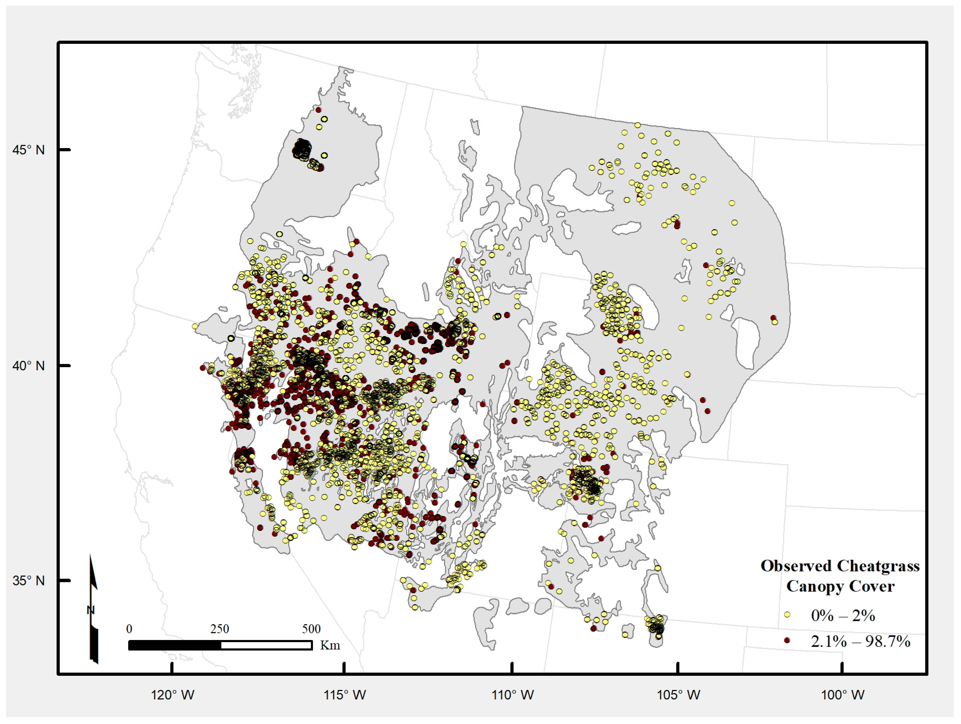
Our goal is to derive more discriminative, higher-resolution models of cheatgrass occurrence using Downs et al. [15] as a starting point. We expand from there by using DL and more traditional machine learning approaches to combine concurrent time series of Landsat-7 ETM+ and MODIS data. Our first objective is to compare the performance of all model types and configurations to identify a single high-performing model configuration. The second objective is to construct a consensus-based ensemble of the preferred model to generate a 30-m ground sample distance (GSD) map of cheatgrass occurrence for the historic range of sage-grouse. The results of this study are intended to provide more detailed information than previously available on the extent of cheatgrass invasion in the western US to support multiple land management agencies’ efforts to mitigate impacts of cheatgrass invasion and facilitate further scientific investigation of factors affecting its spread.

2. Materials and Methods

2.1. Datasets

Three categories of data are used in this study: field observations of cheatgrass cover, time series earth observation satellite data, and biophysical spatial data. We utilize the same labeled field observations and 48 biophysical factors as Downs et al. [15], with the addition of a larger volume of multi-modal satellite data and three ancillary variables. Details about these data and their preparation are described in the following sections.

2.1.1. Field Observations

Downs et al. [15] compiled over 24,000 field vegetation measurements in the historic range of sage-grouse that were collected on multiple unrelated field campaigns between 2001 to 2014 (Figure 1). Of these observations, 6418 are deemed useful based on geographic accuracy and overlap with the study area, completeness, and rigor of collection methods. This was further reduced to 5973 after removing observations that had incomplete satellite data and were less 60-m apart (i.e., the distance of at least two pixels). Nearest-neighbor spacing of field observations ranged from 61 to 79,421-m with a mean distance of 1837-m. Most of the excluded observations are from the U.S. Department of Agriculture (USDA) Forest Inventory and Analysis program, which does not provide the true geographic location of the publicly available version of its data. All field data were collected from transects ranging from 25 m to 100 m in length using point intercept or standardized plot frame techniques.

2.1.2. Satellite Imagery

Time series spectral data from both annual and seasonal composite MODIS Terra [41] and Landsat-7 ETM+ satellites [42] are used in this study (Table 1). Both sets of imagery are composited on a pixel-wise basis to reduce residual cloud and aerosol contamination and reflect the time of peak vegetation vigor as determined by maximum NDVI within the composite period. We use seasonal composite data for the approximate Northern Hemisphere spring (1 March–31 May) and summer (1 June–31 August) periods, which correspond to periods of peak productivity (spring) and senescence (summer) in the life cycle of cheatgrass.
The Landsat-7 annual and seasonal composite data spans most (2003–2012) of the period of selected field observations. We initially used MODIS data for the same period as Landsat-7, but later added annual and seasonal composite data for years 2001–2002 and 2015–2016 because it was found to improve results. In summary, we compiled annual and seasonal composite satellite data corresponding to all years that field observations were collected, except for 2001–2002 and 2014 for which we did not have Landsat-7 data. It is appropriate to use different time phases of satellite data in our models because these data are treated either as independent non-sequential variables or as independent time series in our models. Furthermore, the full temporal stack of satellite data at each sample location is considered in the analysis, not just the year corresponding to when the sample was collected (see Section 2.2).
Google Earth Engine [43] is used to create annual and seasonal maximum NDVI composites from MODIS 16-day composite data and resample it to the spatial resolution of Landsat-7 (30 m GSD). For each MODIS and Landsat-7 composite time series, we also derive a delta-NDVI grid for each year that represents the pixel-wise difference between NDVI and the long-term median NDVI based on all data in the time series. This metric is like that used by Bradley and Mustard [10], who found the delta-NDVI between dry and wet years to be a useful indicator of cheatgrass presence as invaded areas tend to exhibit greater inter-annual NDVI variability than native vegetation.

2.1.3. Biophysical and Ancillary Data

We include the six types of biophysical spatial data used by Downs et al. [15] as well as the ancillary datasets Level-III ecoregions [44], elevation, and gridded latitude and longitude (Table 2). The first biophysical dataset, soil moisture-temperature regimes, is considered because these regimes are known to influence ecosystem resilience and resistance to invasive grasses, including cheatgrass [27,45,46]. These data were derived by Chambers et al. [47] from the SSURGO and STATSGO2 national soils databases and where necessary, we replicated their method to expand its geographic extent to provide complete coverage for our study area.
The second category of biophysical data used is vegetation data derived from the national-scale LANDFIRE Existing Vegetation Type dataset [48]. LANDFIRE vegetation types were generalized into broader plant community associations that are more appropriate for the scale of our analysis and unlikely to change over the time phase of our field observations and satellite data.
Potential relative radiation (PRR) is a unitless index of available solar radiation for photosynthetic activity that is based on solar geometry and terrain and calculated for a specified seasonal period [49]; thus, it is assumed static across years and the time phase of our satellite imagery. PRR is calculated for the same approximate growing season of cheatgrass used in the previous study (i.e., 1 October 2014–30 June 2015).
Growing degree days (GDD) is an index that represents the relative amount of time during a specified period that temperatures are above a given threshold that is considered suitable for growth of the target species [50]. GDD is calculated using the same data and parameters as Downs et al. [15]; i.e., 1-km gridded DAYMET daily minimum and maximum temperature data [51] for 1 October 2014 to 30 April 2015, and a minimum temperature threshold of 0 °C (32 °F). While GDD varies across years due to interannual climate variation, we use a single year to be consistent with the previous study which noted they were primarily interested in representing general geographic patterns of GDD.
The largest, and final, category of biophysical data is a collection of 4-km gridded climatic datasets depicting monthly and annual 30-year (1981–2010) norms for minimum and maximum temperature, and precipitation [52,53] (Table 2). From these data we also derive five seasonal climatic datasets that correspond to important periods during the growing season of cheatgrass: cumulative winter (December–February) precipitation, cumulative spring (April–May) precipitation, cumulative summer (July–August) precipitation, and winter (November–February) minimum and maximum temperature. Seasonal groupings were determined based on expert knowledge and exploratory analysis of cheatgrass occurrence from field data and climatic variables.

2.1.4. Variable Selection

We select four combinations of predictor variables that represent two generic approaches for mapping cheatgrass. The first approach is based on biophysical factors that affect ecological niche and is identical to that used by Downs et al. [15], with the addition of ecoregions and gridded latitude/longitude. The second approach combines ecological niche factors and spectral-spatial remote sensing. The purpose of comparing model performance with these sets is twofold: to evaluate potential gains and losses in classification accuracy by combining ecological and spectral data, and to evaluate gains and losses in classification accuracy by combining data from multiple sensors. For defining variable sets, let x   be the complete set of predictor variables for location i in the study area, and let D p   be a function that selects a defined set of variables from x . The four sets of variables tested are further described in Table 3. All continuous predictor variables are standardized by subtracting their respective mean and dividing by the standard deviation.

2.2. Analysis Methods

Four machine learning methods for predicting cheatgrass occurrence are compared: Random Forest (RF), Logistic Regression (LR), Deep Neural Networks (DNNs), and Joint Recurrent Neural Networks (JRNNs). The classification objective for all models is two classes of cheatgrass occurrence above and below a strong distribution break at 2% cheatgrass canopy cover (Figure 2). This break is selected because it provides a good balance of sample sizes in each class and allows us to avoid the assumption of true absence for sites where cheatgrass was not observed. The LR, DNN, and JRNN models are implemented in Python using the Tensorflow library (version 1.2.1), and RF models are implemented in Python using the Scikit-Learn library (version 0.18.2).

2.2.1. Sampling

Model training and selection is performed using k-fold cross-validation with 90% of the dataset. The other 10% of the data is randomly withdrawn for independent verification. As the data is assimilated from multiple field campaigns that are unevenly distributed throughout time and the study area, there is potential for spatial and temporal autocorrelation. To reduce these effects, samples are randomly shuffled and cross-validation splits are stratified using equal joint distributions based on ecoregion and generalized land cover. Spatial and temporal autocorrelation are further mitigated by ensembling k-fold models as described in Section 2.3.

2.2.2. Categorical Variables

Three categorical variables are included in the models: soil temperature and moisture regime ( c 1 ) , generalized vegetation cover type ( c 2 ) ,   and EPA Level III ecoregions ( c 3 ) (Table 2). As the other inputs to our algorithms are real-valued vectors, we employ two simple strategies for incorporating vector representations of the categorical variables: one-hot vectors in RF models, and embedding vectors for LR, DNN, and JRNN models. One-hot vectors are necessary for incorporating categorical data in RF classifiers. This method can become a limitation when the cardinality of categorical variables is high, causing the dimensionality of the transformed vector to become unmanageable. However, this limitation does not exist in our case because cardinality is low for our categorical variables (i.e., c 1 = 7 ,   c 2 = 15 ,   c 3 = 23 ). For a categorical variable C with k possible classes, for each class, we define a one-hot vector where:
v j = { 1 ,       if   C = j 0 ,       otherwise .
We define v c 1 ,   v c 2 ,   and   v c 3 as the one-hot vectors associated with the categorical values for a location.
Embedding vectors are a parametrized vector representation of categorical values. The values of embedding vectors are learned jointly with the other parameters of the LR, DNN, and JRNN models. We define three embedding matrices for the categorical variables, W c 1   q × 9 , W c 2 q × 15 , and   W c 3   q × 23 where q is the size of the embedding vector, and the second dimension corresponds to the number of classes for a given categorical variable. We define w c 1 ,   w c 2 ,   and   w c 3 as the embedding vectors associated with the categorical values for a location.

2.2.3. Random Forest

The RF method has been shown to perform well for predictive vegetation mapping, is resilient to overfitting, and provides competitive results compared to machine learning approaches in low resource data regimes [54,55,56,57]. To optimize performance of RF models, we performed a search over 200 random RF hyperparameter configurations. Key hyperparameters that we sampled (and their range of values) include: (1) sampling method (with and without replacement); (2) criterion for splitting nodes (GINI index), (3) maximum number of features (square root of the total number of features); (4) minimum number of samples in a leaf node (1, 2, 4); (5) minimum number of samples in a split node (2, 5, 10); (6) maximum depth of a tree (10, 110); and (7) the number of decision trees in the forest (10–200).

2.2.4. Logistic Regression

We include LR as a baseline model in our study because it is used as the classification function in the DNN and JRNN models. With n as the number of continuous variables in the data subset, and q the size of an embedding vector, the input for a given sample is a vector x ^     3 q + n composed of standardized real values of the continuous predictor variables and vector representations of the categorical variables described in Section 2.2.1.
x ^ = [ w c 1   w c 2 w c 3   D p ( x ) ] .
D p is one of the variable selection functions defined in Table 3. The output of the LR model is a vector y ^ 2   containing a probability distribution for the two classes of cheatgrass canopy cover for a given location:
y ^ = s o f t m a x ( W x ^ + b ) ,
where the matrix W 2 × 3 q + n and vector b 2 are learned parameters. The softmax is defined as the elementwise vector-valued function that normalizes elements into a probability distribution:
s o f t m a x ( z ) i = exp ( z i ) j exp ( z j )
We fit the parameters of the logistic regression model by minimizing the cross-entropy between the ground truth and predictions with the ADAM optimization algorithm [58]. ADAM is a variant on the stochastic gradient descent that adjusts the model parameters adaptively according to estimates of the second-order moment of the gradient. We performed 200 training runs with random initializations and random uniform sampled L2 regularization weight (range 0.001–0.1) to select the best LR model.

2.2.5. Deep Learning Models

We evaluate two DL architectures (DNN and JRNN) for mapping cheatgrass. Collectively, these architectures offer a high degree of modeling flexibility for determining the pixel-, object-, or structure-based features, with an added capability of representing all three types of information to express complex relationships [35]. As a universal function approximator, a DNN can derive highly discriminative features that represent complex relationships between input variables in a high dimensional space. In contrast, RNNs (specifically JRNN in this study) can utilize their internal state and flow in multiple directions to exploit sequential connections that may be present in time-series imagery.
The input to the DNN model is the same as defined for the LR model. The architecture of the DNN model (Figure 3) consists of L hidden layers h, which are recursively defined as:
h L = R e L U ( W L h L 1 + b L ) ,
where the ReLU (Rectified Linear Unit) [59] operation is defined as the elementwise vector-valued operation:
R e L U ( z ) i = max ( 0 , z i ) ,
The output of the DNN is directed to a linear LR function (Equation (3)). Dropout normalization is also used to avoid overfitting and reduce generalization error [60], and batch normalization is used to better condition gradient updates [61]. Together, these techniques help to stabilize learning during training.
As an extension to the DNN, we employ a joint composition of bidirectional RNNs, or JRNN, with Long Short Term Memory (LSTM) to predict cheatgrass occurrence (Figure 3). Bidirectional RNNs have been found effective for modeling difficult time-series problems and operate by processing sequence data in both directions, thus allowing output nodes to receive signals from both previous and future time steps [62]. The use of LSTM in an RNN can reduce training difficulties and improve the RNN’s ability to model long-term dependencies [63]. LSTM’s capability to track discriminative values over arbitrary time intervals is especially useful if there are response lags of unknown duration between dependent events in a time-series. Such is the case in this study as the timing and magnitude of cheatgrass growth (and subsequently its detectable presence in time-series spectral-spatial data) may be accelerated or lagged depending on climatic conditions across and within years.
Let X M and X L be MODIS and Landsat-7 time-series, where X t M and X t L are vectors of annual-, spring-, and summer-composite pixel values of the t th year for all spectral bands in Table 1. We define two bidirectional LSTM networks, L S T M M   and L S T M L , for these respective imagery time-series. The LSTMs provide condensed vector representations of the platform time-series for a given location. These vectors are concatenated with the categorical embeddings and the continuous biophysical variables [ D 1 ( x ) ] and used as input to a DNN as previously described but with x ^ as:
x ^ = [ w c 1   w c 2 w c 3   D 1 ( x ) L S T M M ( X M ) L S T M L ( X L ) ]
It is important to note the JRNN cannot be applied with the D1 variable set alone due to the inherent time-series structure of the model.
The parameters of the JRNN and DNN models are fit with the same optimization algorithm, objective function, and regularization strategies as described for the LR model. We perform 200 training runs with random initializations over randomly sampled hyperparameters to identify the best performing DL model configurations. Early stopping based on overall accuracy is used to mitigate overfitting model parameters for all models trained with stochastic gradient descent (LR, DNN, JRNN). The hyperparameters (and their ranges) that we sampled included: number of nodes per hidden layer (32–512 incremented by powers of 2); dropout rate (0–0.5); learn rate (0.001–0.03); and mini-batch size (16–128 incremented by powers of 2).

2.3. Model Ensembling

The resultant probability distributions of cheatgrass occurrence (i.e., ≥2% cheatgrass canopy cover) are strongly bimodal with peaks above and below 0.5; therefore, we use a simple decision rule of p ≥ 0.5 to classify cheatgrass occurrence. Maps of cheatgrass occurrence are produced for each k-fold model from the cross-validation process and ensembled using a simple consensus (or class frequency) method. The method is used to create two types of ensemble maps of cheatgrass occurrence. The first type of ensemble map is a based on the consensus value (0 to 5) and is intended to display spatial agreement among folds. The second type of ensemble map is a binary representation of the first using thresholds ranging from k ≥ 1 to k = 5, which represent less to more restrictive ensemble predictions of cheatgrass occurrence, respectively. This ensemble method is devised to provide insight into the spatial agreement of the individual folds and to identify an optimal ensemble of the folds, as described in the next section.
All predictions are mapped at a 30-m GSD equivalent to that of Landsat-7. Certain portions of the study area corresponding to non-target land cover types (i.e., cultivated lands, pasture and hay, closed canopy deciduous and evergreen forest, urban/developed lands, water) as depicted in the national Cropland Data Layer [64] and National Land Cover Dataset [65] are masked from mapped predictions.

2.4. Model Performance

We use common performance metrics for binary classifiers including overall accuracy, precision, recall, and F1 score (harmonic mean of precision and recall), to evaluate the models and resultant ensemble maps. Acceptable accuracy is defined as >71% observed in our motivating study by Downs et al. [15]. Cross-validation performance is assessed by averaging performance metrics across the k test folds based on 90% of the entire dataset. Verification performance is assessed differently, as shown in Figure 4, due to the use of the consensus method to ensemble the k-fold predictions. Instead, k predictions are made for each verification sample and the consensus level that yields the best overall accuracy or F1 is then reported. In addition, we qualitatively investigate the effect of the consensus method on the performance metrics by plotting overall accuracy and F1 for all five consensus ensembles (i.e., k ≥ 1, k ≥ 2, k ≥ 3, k ≥ 4, k = 5) to determine which consensus level provides the best balance between overall accuracy and F1 (see Section 3.2). We chose to balance performance this way because overall accuracy can be misleading for imbalanced datasets and it helps to balance Type I and Type II error.

2.5. Model Selection

In cases where data are limited, reducing variance in estimators of generalization performance, such as k-fold cross-validation, may be as important as unbiased estimates from independent validation for estimating true generalization performance [66]. Given this consideration, our methods for model selection, and ultimately choosing a high-performing model to map cheatgrass distribution, are intended to accommodate the relatively limited size of our dataset and to independently verify generalization performance of the various methods and resultant map. We tested 10- and 5-fold cross-validation and found 5-fold cross-validation to be the most effective in reducing variance across folds while maintaining acceptable accuracy. Hyperparameters for each model class are chosen according to best average cross-validation accuracy from 200 random hyperparameter sets for each model. Final selection of a model for mapping cheatgrass is subsequently based on cross-validation performance to avoid potential model selection bias. Performance on 10% of the dataset reserved for verification is provided as a theoretically unbiased comparison of performance.

3. Results

The following results relate to our primary objectives as follows: (1) compare the performance of the LR, RF, DNN, and JRNN models tested with four combinations of biophysical and spectral-spatial variables to identify a high-performing model configuration (Section 3.1); and (2) construct a consensus-based ensemble of the preferred model to generate a 30-m GSD map of cheatgrass occurrence (Section 3.2).

3.1. Comparison of Model Types and Variable Sets

All model configurations that we tested demonstrated acceptable (>71%) overall accuracy in cross-validation and verification, except for LR with the biophysical variable set (D1). With this variable set, cross-validation accuracies improved slightly (2–4%) but verification accuracies did not improve relative to the previous study. The best performing models are those that combined Landsat-7 and MODIS with biophysical and ancillary data (D4), achieving cross-validation accuracies that are approximately 7–8% greater than the previous study (Table 4). Among these, the DNN-D4 configuration demonstrated the best cross-validation performance when considering overall accuracy (79.6%), variation in overall accuracy (2.47%; Table 5), and F1 (0.812; Table 6). Verification accuracy of this configuration is very similar (79.1%), suggesting the model is relatively stable when generalizing on unseen data.
While the DL architectures we implemented do enhance prediction of cheatgrass occurrence, we found no apparent trends in overall accuracy (Table 4) or F1 (Table 6) across variable sets that suggests they are superior or inferior to their LR and RF counterparts. Within each variable set the performance advantages of one model type over another are also not strongly distinctive. LR appears to be the slightly stronger model with set D3, although the JRNN achieves a slightly better F1 score with the verification dataset. Similarly, the DNN has slightly better cross-validation performance with D4 than the other models, but RF appears to generalize better with the verification dataset. However, note the verification accuracy of the RF model may be overly optimistic in this case as its cross-validation accuracy is 4.4% lower.
When we evaluate the effects of different variable sets on model performance, we find that adding satellite data (D2, D3, and D4) improves model performance compared to just using biophysical and ancillary data (D1). The differences in overall accuracy (Table 4) and F1 scores (Table 6) between using only MODIS (D2) or only Landsat-7 (D3) are mixed, suggesting there is no obvious advantage of using one sensor in lieu of the other for our application. However, three of the four model types tested (RF, DNN, and JRNN) achieve their best performance when using both sensors (D4). LR achieves its best performance using only Landsat-7 for satellite data (D3).
We later hypothesized that the size of our training dataset (N = 5973) may not have been large enough to provide the DNN and JRNN models a competitive advantage over LR and RF. Recall, we had to discard more than 18,000 field observations due to imprecise geographic accuracy or other quality issues. We qualitatively tested this hypothesis by running the experiments with all the available data (N = 6418). Overall accuracy and F1 from cross-validation was boosted for all model configurations (Table 7), except for LR with set D1 where the F1 score decreased slightly. The DNN and JRNN models became more competitive with RF and LR across variable sets, although this trend is subtle. These findings support our suspicion, although more observation data and rigorous testing is needed to confirm.

3.2. Ensemble Mapping of Cheatgrass Occurrence

As described in Section 2.4, final selection of a model for mapping cheatgrass is based on cross-validation performance due to the limited amount of available data and steps taken to reduce risk of overfitting, model selection bias, and generalization error. Based on this selection criterion, the DNN-D4 configuration is selected to map cheatgrass. We plot trends in DNN-D4 test overall accuracy, F1 score, precision, and recall across all five consensus levels (Figure 5) to examine tradeoffs of our ensembling approach and to identify an appropriate level for post hoc analysis and interpretation. Recall that k ≥ 1 is the least restrictive ensemble and k = 5 is the most restrictive in terms of the predicted area. As we expect, overall accuracy and precision increase as the consensus level becomes more restrictive and false-positives are reduced. Note that overall accuracy becomes unacceptable (<71%) at k ≥ 1 due to poor precision. Overall accuracy peaks (79.1%) at k ≥ 4 due to declining recall and increasing false-negatives, while the balance between precision and recall (F1) peaks at k ≥ 2 (F1 = 0.676). Therefore, we use the midpoint between peak accuracy and peak F1 of k ≥ 3 to produce an accuracy-F1-balanced map of cheatgrass occurrence (Acc. = 78.1%, F1 = 0.673, Prec. = 0.644, Rec. = 0.704; Figure 6).
With this mapped prediction we estimate 253,727-km2 (or 22%) of the historic range of sage-grouse (excluding non-target land cover types as described in Section 2.4) to be invaded by cheatgrass. The effect of balancing accuracy and F1 score on predicted areal extent is evident by comparing Figure 6 and Figure 7, which reveals that even minor differences in ensemble performance can have significant impacts on the estimate of invaded area.
Visual assessment of the cheatgrass maps and zonal analysis by ecoregion (Table 8) confirms that cheatgrass invasion is extensive in the Northern and Central Basin and Range, Snake River Plain, and Columbia Plateau where it has been studied more extensively and is known to be pervasive. Other notable areas of apparent invasion that are less-studied include a region overlapping a southern portion of the Wyoming Basin and the northern portion of the Colorado Plateaus ecoregions, a region in the western portion of the Northwestern Great Plains ecoregion, and a region overlapping the southern portion of the Northwestern Great Plains and northern portion of the High Plains ecoregions.

4. Discussion

This study focused on developing more discriminative, higher-resolution models of cheatgrass occurrence for the historic range of the greater sage-grouse, using Downs et al. [15] as a baseline. In doing so, we were able to improve overall accuracy by approximately 7% and increase spatial resolution from 250- to 30-m GSD, relative to the previous study. We consider these improvements biologically significant because even minor differences in accuracy can result in large differences in predicted areal extents, especially for species that are widespread over large geographic areas like cheatgrass [67,68]. The accuracy of our accuracy-F1-balanced cheatgrass map (78.1%) is comparable to other studies that focused on much smaller regions in the Great Basin, Snake River Plain, and Colorado Plateau. For example, Bradley and Mustard [10] achieved 64% and 72% accuracy, respectively, using AVHRR and Landsat-7. In a related study [12], accuracies ranged from 54% to 74% using Landsat MSS, TM, and ETM+. It is worth noting, however, that these studies predicted more monotypic areas heavily infested with cheatgrass, whereas our study focused on identifying areas with at least 2% canopy cover of cheatgrass. Singh and Glenn [17] achieved 77% accuracy in southern Idaho using Landsat. Bishop et al. [19] reports higher model accuracies (85–92%) for seven national parks in the Colorado Plateau, although it is worth noting these estimates are based on the combined area of low and high probability of occurrence classes where cheatgrass was considered present if it occurred at >10% canopy cover; thus, making interpretation of accuracy difficult. In summary, we find our results encouraging compared to previous studies given the difference in geographic scale and ecological diversity of our study area, as well as lower threshold for detection of cheatgrass occurrence.
Combining biophysical, ancillary, and satellite data generally improved the performance of the four model classes that we tested, lending further credence to approaches for mapping cheatgrass that incorporate ecological niche factors and remote sensing [7,8,11,15,24,25]. Looking more closely at the satellite data, we found that combining concurrent MODIS and Landsat-7 data generally improves model performance compared to using either sensor alone. We attribute this result to choosing sensors with spectral-spatial characteristics that are complimentary to mapping cheatgrass and selecting robust machine learning techniques that are well-suited for deriving discriminative features from multi-modal data. This approach is simpler than fusing satellite data and provides greater flexibility for choosing and testing sensors for a given application. However, we do not discourage data fusion or use of fused satellite data such as HLS [30], which has shown to be useful for mapping exotic annual grass cover [31]. In fact, DL algorithms have shown promise for performing pixel-level image fusion [69]. As such, the combined modeling and data fusion capabilities of DL make it an intriguing tool for leveraging the rapidly increasing volume of EO imagery [38,39].
The similar performance among model architectures in this study underscores the importance of evaluating multiple analysis methods and variable combinations. In a meta-analysis of land cover mapping literature, accuracy differences due to algorithm choice were not found to be as large as those due to the type of data used [70]. While DL algorithms have been proven superior in many remote sensing applications [35,36,37], their performance also hinges on having sufficiently large datasets to learn highly discriminative features in the data. However, what defines “sufficiently large” is not common knowledge and depends on the complexity of the problem and learning algorithm [71]. This topic is considered by some to be one of the major research topics for DL in remote sensing that remains largely unanswered [35]. We did observe a benefit to all models from adding 10% more data, suggesting that sample size may be a limiting factor in our cross-model comparison. The performance of DL models in this study is still encouraging, however, given the circumstances and comparable performance to LR and RF under a limited data regime. This is consistent with others who have shown good performance using DL for similar land use/land-cover applications [71,72,73,74,75]. Acquiring more field data was beyond the scope of this study but should be a priority for future research given that more data has likely become available since the previous study.
We chose relatively simple DL methods as a logical first step to assess whether DL was appropriate for our application and might warrant investigating more computationally intensive methods such as convolutional neural networks (CNNs). CNNs are commonly used in overhead imagery remote sensing due to their ability to take advantage of information in neighboring pixels [36]. However, CNNs may not perform well in cases when the phenomena of interest occur in mixed pixels or exists in the sub-pixel space [74], such as is the case with cheatgrass. Furthermore, the problem can be exacerbated if higher resolution imagery is not available or there is significant cloud cover present. These considerations and greater ease of use of the DNN and JRNN methods factored into our decision to exclude CNN from this study. However, we suggest the relative success of the DNN and JRNN methods does warrant future testing of CNN approaches, and a logical next step might be developing joint DNN-CNN or JRNN-CNN architectures for a semi-supervised classification.

5. Conclusions

In this paper, we propose two straightforward DL approaches (DNN and JRNN) using large predictive variable sets of biophysical and multi-modal remote sensing data (MODIS and Landsat-7 ETM+) to improve prediction (accuracy and spatial resolution) of the invasive exotic annual grass, cheatgrass. We benchmark DL models to two conventional machine learning algorithms (LR and RF) and compare results to a prior study that was an inspiration and data source for this study. Both DL approaches were found to improve prediction, although there was only a slight advantage over LR or RF with our dataset. We surmise that more labeled data is needed to achieve better performance with the DL methods but note the preferred DNN model provided a 7–8% accuracy improvement over the comparison study. The model’s ability to predict cheatgrass occurrence over the historic range of sage-grouse (i.e., much of the western US) with comparable to improved accuracy compared to previous smaller scale studies is also noteworthy. Combining biophysical and multi-modal satellite data was also found to improve the prediction of cheatgrass in all models. A 30-m GSD map of cheatgrass occurrence is produced for the historic range of sage-grouse to help land managers and researchers better understand factors affecting its spread, assess fire risk, and identify and prioritize areas for treatment. We suggest future work explore existing models with additional observation data collected in subsequent years, along with an expansion of remote sensing time-series data. In addition, data augmentation techniques should be explored to increase the total population of training data and other DL architectures should be evaluated for performance improvements.

Author Contributions

Conceptualization, K.B.L.; methodology, K.B.L. and A.R.T.; software, A.R.T.; validation, K.B.L. and A.R.T.; formal analysis, A.R.T.; investigation, K.B.L. and A.R.T.; resources, K.B.L. and A.R.T.; data curation, K.B.L.; writing—original draft preparation, K.B.L. and A.R.T.; writing—review and editing, K.B.L. and A.R.T.; visualization, K.B.L. and A.R.T.; supervision, K.B.L.; project administration, K.B.L.; funding acquisition, K.B.L. and A.R.T. All authors have read and agreed to the published version of the manuscript.

Funding

This research received no external funding.

Institutional Review Board Statement

Not applicable.

Informed Consent Statement

Not applicable.

Data Availability Statement

The data, results, code, and figures presented in this paper are openly available at www.github.com/pnnl/fieryfuture, accessed on 24 March 2021. Biophysical and satellite raster datasets are available on request from the corresponding author.

Acknowledgments

This work was funded by the Deep Learning for Scientific Discovery Laboratory Directed Research and Development investment at the Pacific Northwest National Laboratory (PNNL). PNNL is operated for the United States Department of Energy by Battelle under Contract DE- AC05-76RL01830. We gratefully acknowledge Janelle Downs, Valerie Cullinan, Michael Gregg, Fred Wetzel, and John Klavitter who were instrumental in previous research efforts that provided the basis for this study. This study would not be possible without the collaboration of those who contributed field data, including Lindy Garner, Dave Pyke, Scott Schaff, Dawn-Marie Jensen, the SAGEMap and SageSTEP projects, and the BLM Assessment, Inventory and Monitoring (AIM) program. Thanks to Andre Coleman, Jerry Tagestad, and the anonymous reviewers for providing insightful reviews.

Conflicts of Interest

The authors declare no conflict of interest. The funders had no role in the design of the study; in the collection, analyses, or interpretation of data; in the writing of the manuscript, or in the decision to publish the results.

References

  1. U.S. Department of Agriculture. U.S. Department of Agriculture PLANTS Database. Available online: https://plants.sc.egov.usda.gov/java/ (accessed on 31 March 2019).
  2. Mack, R.N. Invasion of Bromus tectorum L. into western North America: An ecological chronicle. Agro Ecosyst. 1981, 7, 145–165. [Google Scholar] [CrossRef]
  3. Mack, R.N. Fifty Years of ‘Waging War on Cheatgrass’: Research Advances, While Meaningful Control Languishes. In Fifty Years of Invasion Ecology: The Legacy of Charles Elton; Wiley-Blackwell: Oxford, UK, 2011; pp. 253–265. [Google Scholar]
  4. Brooks, M.L.; Matchett, J.R.; Shinneman, D.J.; Coates, P.S. Fire Patterns in the Range of the Greater Sage-Grouse, 1984–2013—Implications for Conservation and Management; Open-File Report 2015-1167; U.S. Geological Survey: Reston, VA, USA, 2015; p. 66. [CrossRef]
  5. Coates, P.S.; Ricca, M.A.; Prochazka, B.G.; Doherty, K.E.; Brooks, M.L.; Casazza, M.L. Long-Term Effects of Wildfire on Greater Sage-Grouse-Integrating Population and Ecosystem Concepts for Management in the Great Basin; Open-File Report 2015-1165; US Geological Survey: Reston, VA, USA, 2015; p. 42. [CrossRef]
  6. Epanchin-Niell, R.; Englin, J.; Nalle, D. Investing in rangeland restoration in the Arid West, USA: Countering the effects of an invasive weed on the long-term fire cycle. J. Environ. Manag. 2009, 91, 370–379. [Google Scholar] [CrossRef] [PubMed]
  7. Boyte, S.P.; Wylie, B.K. Near-Real-Time Cheatgrass Percent Cover in the Northern Great Basin, USA, 2015. Rangelands 2016, 38, 278–284. [Google Scholar] [CrossRef] [Green Version]
  8. Boyte, S.P.; Wylie, B.K.; Major, D.J. Mapping and monitoring cheatgrass dieoff in rangelands of the Northern Great Basin, USA. Rangel. Ecol. Manag. 2015, 68, 18–28. [Google Scholar] [CrossRef]
  9. Boyte, S.P.; Wylie, B.K.; Major, D.J. Cheatgrass Percent Cover Change: Comparing Recent Estimates to Climate Change—Driven Predictions in the Northern Great Basin. Rangel. Ecol. Manag. 2016, 69, 265–279. [Google Scholar] [CrossRef]
  10. Bradley, B.A.; Mustard, J.F. Identifying land cover variability distinct from land cover change: Cheatgrass in the Great Basin. Remote Sens. Environ. 2005, 94, 204–213. [Google Scholar] [CrossRef]
  11. Clinton, N.E.; Potter, C.; Crabtree, B.; Genovese, V.; Gross, P.; Gong, P. Remote Sensing–Based Time-Series Analysis of Cheatgrass (L.) Phenology. J. Environ. Qual. 2010, 39, 955–963. [Google Scholar] [CrossRef]
  12. Bradley, B.A.; Mustard, J.F. Characterizing the Landscape Dynamics of an Invasive Plant and Risk of Invasion Using Remote Sensing. Ecol. Appl. 2006, 16, 1132–1147. [Google Scholar] [CrossRef] [Green Version]
  13. Peterson, E. Estimating cover of an invasive grass (Bromus tectorum) using tobit regression and phenology derived from two dates of Landsat ETM+ data. Int. J. Remote Sens. 2005, 26, 2491–2507. [Google Scholar] [CrossRef]
  14. Schroeder, M.A.; Aldridge, C.L.; Apa, A.D.; Bohne, J.R.; Braun, C.E.; Bunnell, S.D.; Connelly, J.W.; Deibert, P.A.; Gardner, S.C.; Hilliard, M.A.; et al. Distribution of Sage-Grouse in North America. Condor 2004, 106, 363–376. [Google Scholar] [CrossRef]
  15. Downs, J.L.; Larson, K.B.; Cullinan, V.I. Mapping Cheatgrass Across the Range of the Greater Sage-Grouse; Pacific Northwest National Laboratory: Richland, WA, USA, 2016. [Google Scholar] [CrossRef]
  16. Noujdina, N.V.; Ustin, S.L. Mapping Downy Brome (Bromus tectorum) Using Multidate AVIRIS Data. Weed Sci. 2008, 56, 173–179. [Google Scholar] [CrossRef]
  17. Singh, N.; Glenn, N.F. Multitemporal spectral analysis for cheatgrass (Bromus tectorum) classification. Int. J. Remote Sens. 2009, 30, 3441–3462. [Google Scholar] [CrossRef]
  18. West, A.M.; Evangelista, P.H.; Jarnevich, C.S.; Kumar, S.; Swallow, A.; Luizza, M.W.; Chignell, S.M. Using multi-date satellite imagery to monitor invasive grass species distribution in post-wildfire landscapes: An iterative, adaptable approach that employs open-source data and software. Int. J. Appl. Earth Obs. Geoinf. 2017, 59, 135–146. [Google Scholar] [CrossRef]
  19. Bishop, T.B.B.; Munson, S.; Gill, R.A.; Belnap, J.; Petersen, S.L.; Clair, S.B. Spatiotemporal patterns of cheatgrass invasion in Colorado Plateau National Parks. Landsc. Ecol. 2019, 34, 925–941. [Google Scholar] [CrossRef]
  20. Villarreal, M.L.; Soulard, C.E.; Waller, E.K. Landsat Time Series Assessment of Invasive Annual Grasses Following Energy Development. Remote Sens. 2019, 11, 2553. [Google Scholar] [CrossRef] [Green Version]
  21. Waller, E.K.; Villarreal, M.L.; Poitras, T.B.; Nauman, T.W.; Duniway, M.C. Landsat time series analysis of fractional plant cover changes on abandoned energy development sites. Int. J. Appl. Earth Obs. Geoinf. 2018, 73, 407–419. [Google Scholar] [CrossRef]
  22. Bradley, B.A. Regional analysis of the impacts of climate change on cheatgrass invasion shows potential risk and opportunity. Glob. Chang. Biol. 2009, 15, 196–208. [Google Scholar] [CrossRef]
  23. Sherrill, K.; Romme, W. Spatial variation in postfire cheatgrass: Dinosaur National Monument, USA. Fire Ecol. 2012, 8, 38–56. [Google Scholar] [CrossRef]
  24. Boyte, S.P.; Wylie, B.K.; Major, D.J.; Brown, J.F. The integration of geophysical and enhanced Moderate Resolution Imaging Spectroradiometer Normalized Difference Vegetation Index data into a rule-based, piecewise regression-tree model to estimate cheatgrass beginning of spring growth. Int. J. Digit. Earth 2015, 8, 118–132. [Google Scholar] [CrossRef]
  25. Rivera, S.; West, N.E.; Hernandez, A.J.; Ramsey, R.D. Predicting the Impact of Climate Change on Cheat Grass (Bromus tectorum) Invasibility for Northern Utah: A GIS and Remote Sensing Approach. Nat. Resour. Environ. Issues 2011, 17, 95. [Google Scholar]
  26. Rice, K.J.; Black, R.A.; Radamaker, G.; Evans, R.D. Photosynthesis, Growth, and Biomass Allocation in Habitat Ecotypes of Cheatgrass (Bromus tectorum). Funct. Ecol. 1992, 6, 32–40. [Google Scholar] [CrossRef]
  27. Chambers, J.C.; Bradley, B.A.; Brown, C.S.; D’Antonio, C.; Germino, M.J.; Grace, J.B.; Hardegree, S.P.; Miller, R.F.; Pyke, D.A. Resilience to stress and disturbance, and resistance to Bromus tectorum L. invasion in cold desert shrublands of western North America. Ecosystems 2014, 17, 360–375. [Google Scholar] [CrossRef]
  28. Bradford, J.B.; Lauenroth, W.K. Controls over invasion of Bromus tectorum: The importance of climate, soil, disturbance and seed availability. J. Veg. Sci. 2006, 17, 693–704. [Google Scholar] [CrossRef] [Green Version]
  29. Stohlgren, T.J.; Ma, P.; Kumar, S.; Rocca, M.; Morisette, J.T.; Jarnevich, C.S.; Benson, N. Ensemble Habitat Mapping of Invasive Plant Species. Risk Anal. 2010, 30, 224–235. [Google Scholar] [CrossRef] [PubMed]
  30. Claverie, M.; Ju, J.; Masek, J.G.; Dungan, J.L.; Vermote, E.F.; Roger, J.-C.; Skakun, S.V.; Justice, C. The Harmonized Landsat and Sentinel-2 surface reflectance data set. Remote Sens. Environ. 2018, 219, 145–161. [Google Scholar] [CrossRef]
  31. Pastick, N.J.; Dahal, D.; Wylie, B.K.; Parajuli, S.; Boyte, S.P.; Wu, Z. Characterizing Land Surface Phenology and Exotic Annual Grasses in Dryland Ecosystems Using Landsat and Sentinel-2 Data in Harmony. Remote Sens. 2020, 12, 725. [Google Scholar] [CrossRef] [Green Version]
  32. Yuan, Q.; Shen, H.; Li, T.; Li, Z.; Li, S.; Jiang, Y.; Xu, H.; Tan, W.; Yang, Q.; Wang, J.; et al. Deep learning in environmental remote sensing: Achievements and challenges. Remote Sens. Environ. 2020, 241, 111716. [Google Scholar] [CrossRef]
  33. Lary, D.J.; Alavi, A.H.; Gandomi, A.H.; Walker, A.L. Machine learning in geosciences and remote sensing. Geosci. Front. 2016, 7, 3–10. [Google Scholar] [CrossRef] [Green Version]
  34. Ma, L.; Liu, Y.; Zhang, X.; Ye, Y.; Yin, G.; Johnson, B.A. Deep learning in remote sensing applications: A meta-analysis and review. Isprs J. Photogramm. Remote Sens. 2019, 152, 166–177. [Google Scholar] [CrossRef]
  35. Zhang, L.; Zhang, L.; Du, B. Deep Learning for Remote Sensing Data: A Technical Tutorial on the State of the Art. IEEE Geosci. Remote Sens. Mag. 2016, 4, 22–40. [Google Scholar] [CrossRef]
  36. Zhu, X.X.; Tuia, D.; Mou, L.; Xia, G.; Zhang, L.; Xu, F.; Fraundorfer, F. Deep Learning in Remote Sensing: A Comprehensive Review and List of Resources. IEEE Geosci. Remote Sens. Mag. 2017, 5, 8–36. [Google Scholar] [CrossRef] [Green Version]
  37. Li, J.; Huang, X.; Gong, J. Deep neural network for remote-sensing image interpretation: Status and perspectives. Natl. Sci. Rev. 2019, 1–4. [Google Scholar] [CrossRef]
  38. Lee, J.-G.; Kang, M. Geospatial Big Data: Challenges and Opportunities. Big Data Res. 2015, 2, 74–81. [Google Scholar] [CrossRef]
  39. Nativi, S.; Mazzetti, P.; Santoro, M.; Papeschi, F.; Craglia, M.; Ochiai, O. Big Data challenges in building the Global Earth Observation System of Systems. Environ. Model. Softw. 2015, 68, 1–26. [Google Scholar] [CrossRef]
  40. Reichstein, M.; Camps-Valls, G.; Stevens, B.; Jung, M.; Denzler, J.; Carvalhais, N.; Prabhat. Deep learning and process understanding for data-driven Earth system science. Nature 2019, 566, 195–204. [Google Scholar] [CrossRef]
  41. Didan, K. MOD13Q1 MODIS/Terra Vegetation Indices 16-Day L3 Global 250 m SIN Grid V006. NASA Earth Obs. Syst. Data Inf. Syst. LP DAAC. 2015. [Google Scholar] [CrossRef]
  42. Roy, D.P.; Ju, J.; Kline, K.; Scaramuzza, P.L.; Kovalskyy, V.; Hansen, M.; Loveland, T.R.; Vermote, E.; Zhang, C. Web-enabled Landsat Data (WELD): Landsat ETM+ composited mosaics of the conterminous United States. Remote Sens. Environ. 2010, 114, 35–49. [Google Scholar] [CrossRef]
  43. Gorelick, N.; Hancher, M.; Dixon, M.; Ilyushchenko, S.; Thau, D.; Moore, R. Google Earth Engine: Planetary-scale geospatial analysis for everyone. Remote Sens. Environ. 2017, 202, 18–27. [Google Scholar] [CrossRef]
  44. Omernik, J.M.; Griffith, G.E. Ecoregions of the Conterminous United States: Evolution of a Hierarchical Spatial Framework. Environ. Manag. 2014, 54, 1249–1266. [Google Scholar] [CrossRef]
  45. Chambers, J.C.; Pyke, D.A.; Maestas, J.D.; Pellant, M.; Boyd, C.S.; Campbell, S.B.; Espinosa, S.; Havlina, D.W.; Mayer, K.E.; Wuenschel, A. Using Resistance and Resilience Concepts to Reduce Impacts of Invasive Annual Grasses and Altered Fire Regimes on the Sagebrush Ecosystem and Greater Sage-Grouse: A Strategic Multi-Scale Approach; General Technical Report RMRS-GTR-326; USDA Forest Service: Fort Collins, CO, USA, 2014; p. 73. [CrossRef]
  46. Chambers, J.C.; Roundy, B.A.; Blank, R.R.; Meyer, S.E.; Whittaker, A. What makes Great Basin sagebrush ecosystems invasible by Bromus tectorum? Ecol. Monogr. 2007, 77, 117–145. [Google Scholar] [CrossRef] [Green Version]
  47. Chambers, J.C.; Miller, R.F.; Board, D.I.; Pyke, D.A.; Roundy, B.A.; Grace, J.B.; Schupp, E.W.; Tausch, R.J. Resilience and resistance of sagebrush ecosystems: Implications for state and transition models and management treatments. Rangel. Ecol. Manag. 2014, 67, 440–454. [Google Scholar] [CrossRef] [Green Version]
  48. U.S. Geological Survey Wildland Fire Science. LANDFIRE Existing Vegetation Type (LANDFIRE.US_130EVT). 2013. Available online: https://www.landfire.gov/evt.php (accessed on 1 October 2018).
  49. Pierce, K.B.; Lookingbill, T.; Urban, D. A simple method for estimating potential relative radiation (PRR) for landscape-scale vegetation analysis. Landsc. Ecol. 2005, 20, 137–147. [Google Scholar] [CrossRef]
  50. Ball, D.A.; Frost, S.M.; Gitelman, A.I. Predicting timing of downy brome (Bromus tectorum) seed production using growing degree days. Weed Sci. 2004, 52, 518–524. [Google Scholar] [CrossRef]
  51. Thornton, P.E.; Thornton, M.M.; Mayer, B.W.; Wilhelmi, N.; Wei, Y.; Devarakonda, R.; Cook, R.B. Daymet: Daily Surface Weather Data on a 1-km Grid for North America, Version 2. Distrib. Act. Arch. Cent. 2014. [Google Scholar] [CrossRef]
  52. Daly, C.; Halbleib, M.; Smith, J.I.; Gibson, W.P.; Doggett, M.K.; Taylor, G.H.; Curtis, J.; Pasteris, P.P. Physiographically sensitive mapping of climatological temperature and precipitation across the conterminous United States. Int. J. Climatol. 2008, 28, 2031–2064. [Google Scholar] [CrossRef]
  53. PRISM Climate Group. United States Average Annual Precipitation, 1981–2010 (4 km). 2012. Available online: http://www.prism.oregonstate.edu/normals (accessed on 1 October 2018).
  54. Belgiu, M.; Drăguţ, L. Random forest in remote sensing: A review of applications and future directions. Isprs J. Photogramm. Remote Sens. 2016, 114, 24–31. [Google Scholar] [CrossRef]
  55. Cutler, D.R.; Edwards, T.C.; Beard, K.H.; Cutler, A.; Hess, K.T.; Gibson, J.; Lawler, J.J. Random forests for classification in ecology. Ecology 2007, 88, 2783–2792. [Google Scholar] [CrossRef]
  56. Pal, M. Random forest classifier for remote sensing classification. Int. J. Remote Sens. 2005, 26, 217–222. [Google Scholar] [CrossRef]
  57. Rodriguez-Galiano, V.F.; Ghimire, B.; Rogan, J.; Chica-Olmo, M.; Rigol-Sanchez, J.P. An assessment of the effectiveness of a random forest classifier for land-cover classification. Isprs J. Photogramm. Remote Sens. 2012, 67, 93–104. [Google Scholar] [CrossRef]
  58. Kingma, D.P.; Ba, J.L. ADAM: A method for stochastic optimization. In Proceedings of the International Conference on Learning Representations (ICLR), San Diego, CA, USA, 5–8 May 2015; p. 15. [Google Scholar]
  59. Nair, V.; Hinton, G.E. Rectified linear units improve restricted boltzmann machines. In Proceedings of the 27th International Conference on International Conference on Machine Learning, Haifa, Israel, 21–24 June 2010; pp. 807–814. [Google Scholar]
  60. Srivastava, N.; Hinton, G.; Krizhevsky, A.; Stuskever, I.; Salakhutdinov, R. Dropout: A Simple Way to Prevent Neural Networks from Overfitting. J. Mach. Learn. Res. 2014, 15, 1929–1958. [Google Scholar] [CrossRef]
  61. Ioffe, S.; Szegedy, C. Batch Normalization: Accelerating Deep Network Training by Reducing Internal Covariate Shift. In Proceedings of the International Conference on Machine Learning (ICML), Lille, France, 6–11 July 2015; p. 11. [Google Scholar]
  62. Schuster, M.; Paliwal, K.K. Bidirectional recurrent neural networks. IEEE Trans. Signal Process. 1997, 45, 2673–2681. [Google Scholar] [CrossRef] [Green Version]
  63. Hochreiter, S.; Schmidhuber, J. Long short-term memory. Neural Comput. 1997, 9, 1735–1780. [Google Scholar] [CrossRef] [PubMed]
  64. USDA National Agricultural Statistics Service. Published Crop-Specific Data Layer. 2016. Available online: https://nassgeodata.gmu.edu/CropScape/ (accessed on 3 April 2016).
  65. Jin, S.; Yang, L.; Danielson, P.; Homer, C.; Fry, J.; Xian, G. NLCD 2011 Land Cover; 2011 Edition; amended 2014 ed.; U.S. Geological Survey: Sioux Falls, SD, USA, 2014. [CrossRef]
  66. Cawley, G.C.; Talbot, N.L.C. On over-fitting in model selection and subsequent selection bias in performance evaluation. J. Mach. Learn. Res. 2010, 11, 2079–2107. [Google Scholar]
  67. Huang, Q.; Fleming, C.H.; Robb, B.; Lothspeich, A.; Songer, M. How different are species distribution model predictions?—Application of a new measure of dissimilarity and level of significance to giant panda Ailuropoda melanoleuca. Ecol. Inform. 2018, 46, 114–124. [Google Scholar] [CrossRef]
  68. McPherson, J.M.; Jetz, W.; Rogers, D.J. The effects of species’ range sizes on the accuracy of distribution models: Ecological phenomenon or statistical artefact? J. Appl. Ecol. 2004, 41, 811–823. [Google Scholar] [CrossRef]
  69. Liu, Y.; Chen, X.; Wang, Z.; Wang, Z.J.; Ward, R.K.; Wang, X. Deep learning for pixel-level image fusion: Recent advances and future prospects. Inf. Fusion 2018, 42, 158–173. [Google Scholar] [CrossRef]
  70. Yu, L.; Liang, L.; Wang, J.; Zhao, Y.; Cheng, Q.; Hu, L.; Liu, S.; Yu, L.; Wang, X.; Zhu, P.; et al. Meta-discoveries from a synthesis of satellite-based land-cover mapping research. Int. J. Remote Sens. 2014, 35, 4573–4588. [Google Scholar] [CrossRef]
  71. Cheng, G.; Li, Z.; Han, J.; Yao, X.; Guo, L. Exploring Hierarchical Convolutional Features for Hyperspectral Image Classification. IEEE Trans. Geosci. Remote Sens. 2018, 56, 6712–6722. [Google Scholar] [CrossRef]
  72. Chen, Y.; Lin, Z.; Zhao, X.; Wang, G.; Gu, Y. Deep Learning-Based Classification of Hyperspectral Data. IEEE J. Sel. Top. Appl. Earth Obs. Remote Sens. 2014, 7, 2094–2107. [Google Scholar] [CrossRef]
  73. Kussul, N.; Lavreniuk, M.; Skakun, S.; Shelestov, A. Deep Learning Classification of Land Cover and Crop Types Using Remote Sensing Data. IEEE Geosci. Remote Sens. Lett. 2017, 14, 778–782. [Google Scholar] [CrossRef]
  74. Zhang, M.; Lin, H.; Wang, G.; Sun, H.; Fu, J. Mapping Paddy Rice Using a Convolutional Neural Network (CNN) with Landsat 8 Datasets in the Dongting Lake Area, China. Remote Sens. 2018, 10, 1840. [Google Scholar] [CrossRef] [Green Version]
  75. Zhao, W.; Du, S. Learning multiscale and deep representations for classifying remotely sensed imagery. Isprs. J. Photogramm. Remote Sens. 2016, 113, 155–165. [Google Scholar] [CrossRef]
Figure 1. Distribution of field vegetation measurements (points) within the historic range of sage-grouse (gray area). For reference, field measurements are colored by their observed canopy cover values binned into the classes used in our classification.
Remotesensing 13 01246 g001
Figure 2. Cumulative probability distribution of cheatgrass canopy cover at field sample locations. The red line illustrates a strong break at 2% canopy cover and is used to define cover classes for this study.
Remotesensing 13 01246 g002
Figure 3. Combined depiction of the DNN and JRNN architectures. In the DNN-only configuration, the set of continuous [Dp(x)] and categorical ( w c 1 ,   w c 2 ,   w c 3 ) predictors (Equation (2)) are provided as input x ^ . In the JRNN configuration, the condensed vector representations of imagery time-series created by the joint LSTM networks are concatenated with the D1(x) set of continuous biophysical variables and categorical ( w c 1 ,   w c 2 ,   w c 3 ) predictors (Equation (7)) to create an input x ^ to the DNN.
Remotesensing 13 01246 g003
Figure 4. Process diagram illustrating how cross-validation and verification performance metrics (E) are assessed. Beginning in the upper right, the dataset is split into training and verification sets. During cross-validation, five iterations of a model ( M i ) are trained and tested on different folds of the training set and performance ( E i ) is averaged across folds ( E ¯ ). Conversely, verification performance is assessed by ensembling the predictions from each of the k-fold models ( M i ) using the consensus method, which yields k estimates performance ( E k ). This same process is applied to each map pixel.
Remotesensing 13 01246 g004
Figure 5. Verification overall accuracy, F1 score, precision, and recall across k-fold consensus levels for the DNN-D4 model figuration. The horizontal dashed line indicates our threshold for acceptable accuracy (>71%).
Remotesensing 13 01246 g005
Figure 6. Predicted distribution of cheatgrass occurrence (>2% canopy cover) in the historic range of sage-grouse (excluding areas classified as non-target land cover types) depicted as: (a) the spatial agreement (i.e., consensus of k-fold predictions), and (b) accuracy-F1-balanced consensus of k ≥ 3 overlaid by EPA Level-III ecoregion boundaries (numbering corresponds to ecoregion names in Table 8).
Remotesensing 13 01246 g006aRemotesensing 13 01246 g006b
Figure 7. Cumulative areas (blue dots) and proportions (red squares) of the predicted area occupied by cheatgrass for each k-fold consensus level.
Remotesensing 13 01246 g007
Table 1. MODIS and Landsat-7 ETM+ spectral bands and indices used in this study.
SensorSpectral Bands/Indices
MODIS TerraNDVI, EVI, Blue, Red, Near-infrared, Mid-infrared, Delta-NDVI, Median NDVI
Landsat-7 ETM+Blue, Green, Red, Near-infrared, Shortwave infrared 1, Low-gain thermal, High-gain thermal, Shortwave Infrared 2, Delta-NDVI, Median NDVI
Table 2. Categorical (ci) and continuous (xi) biophysical, ancillary, and spectral predictor variables included in variable sets.
Variable NotationDescription
c1Soil temperature and moisture regime classes
c2Generalized vegetation cover type
c3EPA Level III Ecoregions
x1:230-m gridded latitude and longitude
x3Elevation above mean sea level
x4Potential Relative Radiation
x5Median winter precipitation
x6Median growing degree days
x7:5030-year normal climatic conditions
x51:324Landsat-7 bands 1–10 (annual, spring, summer)
x325:666MODIS Terra bands 1–8 (annual, spring, summer)
Table 3. Sets of continuous predictor variables used in all models.
Variable Set NotationSelected VariablesDescription
D 1 x1:50Biophysical and ancillary variables
D 2 x1:50, 325:666Biophysical, ancillary, and MODIS variables
D 3 x1:324Biophysical, ancillary, and Landsat variables
D 4 x1:666All variables (biophysical, ancillary, MODIS, Landsat)
Table 4. Overall accuracy (%) of cross-validation (CV) and verification (V) across model types and variable sets. The k-fold consensus threshold that yields the best verification accuracy is denoted in superscripts.
Variable SetD1D2D3D4
ModelCVVCVVCVVCVV
LR75.769.6 k≥478.074.6 k=578.782.0 k=578.678.3 k=5
RF73.871.8 k=577.882.0 k≥477.480.3 k=578.482.8 k≥4
DNN75.072.0 k=578.276.8 k=578.580.2 k=579.679.1 k≥4
JRNN----76.281.9 k=576.480.3 k=577.280.8 k=5
Table 5. Standard deviation of cross-validation overall accuracy (%) across model types and variable sets.
Variable SetD1D2D3D4
LR2.682.902.502.75
RF4.583.072.212.53
DNN2.822.811.382.47
JRNN 2.132.151.98
Table 6. Cross-validation (CV) and test F1 scores across model types and variable sets. The k-fold consensus threshold that yields the best verification F1 score is denoted in superscripts.
Variable SetD1D2D3D4
ModelCVVCVVCVVCVV
LR0.7850.617 k≥30.8020.586 k≥20.8080.703 k=50.8050.661 k≥3
RF0.7570.638 k≥30.7960.722 k≥40.7940.706 k=50.8020.733 k≥4
DNN0.7760.639 k≥30.7980.634 k≥30.8040.706 k≥30.8120.677 k≥2
JRNN----0.7830.710 k≥30.7840.717 k=50.7930.719 k=5
Table 7. Overall accuracy (%) and F1 scores from cross-validation using all available field observations.
Variable SetD1D2D3D4
ModelAcc.F1Acc.F1Acc.F1Acc.F1
LR76.70.76879.60.80881.20.82281.40.822
RF80.20.81181.70.82482.50.83382.80.835
DNN79.60.80882.00.82382.50.83283.20.839
JRNN----82.10.82882.70.83583.20.840
Table 8. Predicted areal extents of cheatgrass occurrence by ecoregion based on k ≥ 3 spatial consensus. For reference, the total and masked areas of the historic range of sage-grouse are provided. The proportion of cheatgrass occupied area is relative to the masked area of the sage-grouse range. The numbering of ecoregions corresponds to map labels in Figure 6b.
Sage-Grouse Range (km2)Cheatgrass Occupied
EcoregionTotalMaskedTotal (km2)Proportion
1. Arizona/New Mexico Mountains2817110.69
2. Arizona/New Mexico Plateau11,405986315110.15
3. Blue Mountains28,69622,57547580.21
4. Canadian Rockies913900.00
5. Cascades17249240.49
6. Central Basin and Range208,624164,63276,8010.47
7. Colorado Plateaus59,40334,15415,2140.45
8. Columbia Plateau72,14535,31728,9360.82
9. Eastern Cascades Slopes and Foothills17,74410,23856610.55
10. High Plains11,460883968660.78
11. Idaho Batholith3851264213720.52
12. Middle Rockies61,18739,9387320.02
13. Mojave Basin and Range1716154110510.68
14. North Cascades6934381440.33
15. Northern Basin and Range138,180122,50358,0630.47
16. Northern Rockies372417573320.19
17. Northwestern Glaciated Plains83,23542,45414950.04
18. Northwestern Great Plains237,307186,03520,0320.11
19. Sierra Nevada155310907070.65
20. Snake River Plain52,00430,36820,2570.67
21. Southern Rockies28,91416,08212040.07
22. Wasatch and Uinta Mountains17,418893422750.25
23. Wyoming Basin130,732116,34862780.05
Total1,170,280855,852253,727
Publisher’s Note: MDPI stays neutral with regard to jurisdictional claims in published maps and institutional affiliations.

