Hyperspectral Image Classification via Multi-Feature-Based Correlation Adaptive Representation

Abstract

In recent years, representation-based methods have attracted more attention in the hyperspectral image (HSI) classification. Among them, sparse representation-based classifier (SRC) and collaborative representation-based classifier (CRC) are the two representative methods. However, SRC only focuses on sparsity but ignores the data correlation information. While CRC encourages grouping correlated variables together but lacks the ability of variable selection. As a result, SRC and CRC are incapable of producing satisfied performance. To address these issues, in this work, a correlation adaptive representation (CAR) is proposed, enabling a CAR-based classifier (CARC). Specifically, the proposed CARC is able to explore sparsity and data correlation information jointly, generating a novel representation model that is adaptive to the structure of the dictionary. To further exploit the correlation between the test samples and the training samples effectively, a distance-weighted Tikhonov regularization is integrated into the proposed CARC. Furthermore, to handle the small training sample problem in the HSI classification, a multi-feature correlation adaptive representation-based classifier (MFCARC) and MFCARC with Tikhonov regularization (MFCART) are presented to improve the classification performance by exploring the complementary information across multiple features. The experimental results show the superiority of the proposed methods over state-of-the-art algorithms.

1. Introduction

Hyperspectral images (HSIs) provide valuable spectral information by using the hyperspectral imaging sensors to capture data at hundreds of narrow contiguous bands from the same spatial location. In the past few years, HSIs have been extensively applied in various fields [1,2,3,4,5]. Among them, HSI classification is a crucial task for a wide variety of real-world applications, such as ecological science, mineralogy, and precision agriculture [6]. However, there exist open challenges in the HSI classification task. For example, although the hundreds of spectral bands provide sufficient information, it results in the Hughes phenomenon. Additionally, given that the practical sample labeling is difficult and expensive, lacking sufficient labeled samples is another major challenge in HSI classification techniques.

In recent years, deep-learning-based techniques have aroused broad interests in the geoscience and remote sensing community. It shows the effectiveness in HSI classification due to a powerful ability of learning high-level and abstract features from the HSI data automatically [7]. Compared with traditional classification methods, deep learning-based approaches normally require higher computation power and a larger number of training samples to learn the massive tuning parameters, resulting from the manner in deep hierarchical networks [8]. According to the fact that available training samples are limited in hyperspectral data, it is still challenging to use deep learning approaches to fulfill the HSI classification task with high accuracy.

Currently, representation-based classification methods have been successfully applied to HSI classification and numerous representation-based classifiers have been investigated extensively. Started by Wright et al. [9], sparse representation-based classifier (SRC) was proposed for face recognition. Later on, Chen et al. [10] explored a joint sparse representation model into the HSI classification. In recent years, many variants of SRC have been designed for the HSI classification, such as joint SRC (JSRC) [11,12], robust SRC (RSRC) [13] and group SRC (GSRC) [14,15]. Zhang et al. [16] investigated the core principle of SRC and asserted that it was the collaborative representation (CR) mechanism deduced by ${\ell }_2-\mathrm{norm}$ ${\mathrm{l}}_2-\mathrm{norm}$ rather than the ${\ell }_1-\mathrm{norm}$ ${\mathrm{l}}_1-\mathrm{norm}$ based sparsity constraint to improve the final classification performance. Similar to the query-adapted technique adopted in weighted SRC (WSRC) [17], the nearest regularized subspace (NRS) [18] was presented by introducing the distance-weighted Tikhonov regularization into CRC. Then the CR with Tikhonov regularization (CRT) [19] and different kernel versions of CRC and CRT [20,21,22] were introduced in the HSI classification.

According to the above-mentioned discussion, for the representation-based classifiers, one of the crucial issues is to seek for a suitable representation for any test sample and derive the discriminative representation coefficients to achieve the subsequent classification task. Note, when applying SRC to hyperspectral data, whether a useful sparse solution can be obtained or not mostly depends on the degree of coherence of the dictionary [23]. Specifically, when the samples from the same subspace within the dictionary are highly correlated, SR tends to select one atom at random for representation and overlooks other correlated atoms. It leads to SR suffering from the instability problem. Besides, SR lacks the ability to reveal the correlation structure of the dictionary due to the sparsity [24]. On the other hand, when applying CRC to the HSI classification, CR tends to group correlated samples together but lacks the ability of sample selection, which potentially introduces the between-class interference, resulting in poor classification performance.

Given that both SR and CR have their intrinsic limitations, there are some attempts to achieve the balance between SR and CR for better performance. Li et al. [25] presented a fused representation-based classifier (FRC) by combining SR and CR in the spectral residual domain and Gan et al. [26] developed a kernel version of FRC (KFRC) to attain the balance in the kernel residual domain. Liu et al. [27] extended the KFRC from the spectral kernel residual domain to the composite kernel with ideal regularization (CKIR)-based residual domain to further enhance the class separability. Although these fusion-based classifiers have been demonstrated to perform better than the individual representation-based classifiers, they still cannot perform sample selection and group correlated samples simultaneously. As a remedy, the elastic net representation (ENR) model [24] was proposed to encourage the sparsity and the grouping effect via a combination of the LASSO and the Ridge regression. Inspired from the elastic net, several variants of the ENR-based classification methods have been developed for HSIs to take full advantages of SRC and CRC [28,29,30]. However, the ENR model benefits from both the ${\ell }_1-\mathrm{penalty}$ and the ${\ell }_2-\mathrm{penalty}$ at the cost of having two regularization parameters to tune. In addition, the ENR model is blind to the exact correlation structure of the data and thus fails to balance between SR and CR adaptively according to the precise correlation structure of the dictionary.

To tackle the above-mentioned issues, in this paper, a correlation adaptive representation (CAR) solution and CAR-based classifier (CARC) are proposed by exploring the precise correlation structure of the dictionary effectively. Specifically, we introduce a data correlation adaptive penalty by utilizing the advantage of the correlation adaptive behavior and thus make the model adaptive to the correlation structure of the dictionary. Different from ENR-based classifiers, the proposed CARC is capable of performing sample selection and grouping correlated samples jointly with a single regularization parameter to be tuned. By capturing the correlation structure of data samples, the CARC is able to balance SR and CR adaptively, producing more discriminative representation coefficients for the classification task.

Moreover, as an effective solution to the small training samples issue in HSI classification techniques, the multi-task representation mechanism is employed by integrating the discriminative capabilities of complementary features to augment the training samples [31,32]. As a result, it leads to a new trend to exploit the complementarity contained in multi-feature for the HSI classification [33]. Zhang et al. [34] and Jia et al. [35] respectively proposed a multi-feature joint SRC (MF-JSRC) and a 3-D Gabor cube selection based multitask joint SRC model for hyperspectral data. Fang et al. [36] presented a multi-feature based adaptive sparse representation (MFASR) method to exploit the correlations among features. He et al. [37,38] introduced a class-oriented multitask learning based classifier and a kernel low-rank multitask learning (KL-MTL) method to handle multiple features. To deal with the nonlinear distribution of multiple features, Gan et al. [39] developed a multiple feature kernel SRC for HSI classification. Although these multi-feature based classification algorithms employ the multi-task representation mechanism to improve the classification accuracy, the traditional representation models lead to unsatisfactory performance.

In this paper, a multi-feature correlation adaptive representation-based classifier (MFCARC) is proposed to enhance the classification accuracy under the small size samples situations by employing the multi-task representation mechanism. More importantly, the distance-weighted Tikhonov regularization is introduced to MFCARC, namely, multi-feature correlation adaptive representation with Tikhonov regularization (MFCART) classifier, leading to better performance. The main contributions are summarized as follows.

• A new representation-based classifier CARC is proposed to possess the ability of performing sample selection and grouping correlated samples together simultaneously. It overcomes the intrinsic limitations of the traditional SRC & CRC methods and makes the model balance between SR & CR adaptively according to the precise correlation structure of the dictionary.
• A dissimilarity-weighted Tikhonov regularization is integrated into the MFCARC framework to integrate the locality structure information and encode the correlation between the test sample and the training samples effectively, revealing the true geometry of feature space and thus further improving the class separability.
• A multi-task representation strategy is incorporated into CARC and a correlation adaptive representation with Tikhonov regularization (CART) classifier, respectively, enhancing the classification accuracy under the small size samples situations.

The rest of this paper is organized as follows. Section 2 briefly introduces the extraction of multiple features and the conventional representation-based classifiers. In Section 3, the proposed MFCARC and MFCART algorithms are described. The experimental results on real hyperspectral datasets are present in Section 4. Section 5 provides a discussion of the results and conclusions are drawn in Section 6.

2. Preliminaries

2.1. Multiple Feature Extraction

To provide a comprehensive description of 3-D cube HSIs, we extract four complementary spectral-spatial features from HSIs, i.e., the spectral value feature, the Gabor texture feature, the differential morphological profile (DMP) feature and the local binary pattern (LBP) feature, respectively. The description and extraction of the four features are introduced as follows.

2.1.1. Spectral Value Feature

Spectral feature is used to extract the detailed spectral information. The spectral feature of each hyperspectral pixel is a vector of B elements, with each element corresponding to the spectral value of each band and B denoting the number of all spectral bands.

2.1.2. Gabor Texture Feature

The Gabor wavelet filter has been extensively used in the HSI analysis due to the ability of providing a global description of spatial texture information [40,41]. As an orientation-dependent bandpass filter, its impulse response can be defined by an elliptical Gaussian envelope and a complex plane wave. In a 2-D $\left(x, y\right)$ coordinate system, the Gabor filter can be defined as

$$G_{\delta ,\theta ,\psi ,\sigma ,\gamma }(x,y)=\exp (-\frac{x_{}^{\prime 2}+{\gamma }_{}^2{y}_{}^{\prime 2}}{2{\sigma }_{}^2})\exp (j(2\pi \frac{x_{}^{\prime }}{\delta }+\psi ))$$

(1)

where

$$x_{}^{\prime }=xcos\theta +ysin\theta$$

(2)

$$y_{}^{\prime }=-xsin\theta +ycos\theta$$

(3)

where $\delta$ denotes the wavelength of the sinusoidal factor, $\theta$ represents the orientation separation angle of Gabor kernels, and $\psi$ is the phase offset of the Gabor function. Besides, the real component and the imaginary component of the Gabor filter can be obtained when $\psi =0$ and $\psi =\frac{\pi }{2}$, respectively. $\gamma$ is the spatial aspect ratio used to give the ellipticity of the Gabor function. The standard derivation of the Gaussian envelope is denoted by $\sigma .$ For the given wavelength $\delta$ and the spatial frequency bandwidth $bw$, the parameter $\sigma$ can be calculated as

$$\sigma = \frac{\delta }{\pi }\sqrt{\frac{\ln 2}{2}}\frac{2^{bw} + 1}{2^{bw}-1}.$$

(4)

Subsequently, the designed Gabor filter can be utilized to extract the Gabor texture feature by performing the 2-D Gabor wavelet transform on the selected principle components (PCs) of the HSI. By stacking the Gabor features calculated from each PC, the final Gabor feature for each hyperspectral pixel can be obtained.

2.1.3. Differential Morphological Profile (DMP)

As an effective tool for extracting structural information from HSIs, Morphological profiles (MPs) [42] can be constructed by implementing a series of morphological opening and closing operators with a group of structuring elements (SEs) of increasing sizes. By calculating the slopes of the MPs, DMP can be obtained to represent the shape information. Then DMP features are extracted from several PCs of the HSIs. Specifically, we apply the DMP on the selected PCs in a sequential way to yield the DMP feature.

Let ${\Upsilon }^{\mathrm{SE}}\left({pc}_{\mathrm{i}}\right)$ and ${\varphi }^{\mathrm{SE}}({pc}_i)$ denote the morphological opening operator and closing operator by reconstruction using the SEs for each selected PC image ${pc}_i$, where ${pc}_i$ represents the $i\mathrm{th}$ PC of the HSI. The definition of MPs is based on a series of SEs with increasing sizes.

$${\mathrm{MP}}_{\mathsf{\Upsilon } }= \{{\mathrm{MP}}_{\mathsf{\Upsilon }}^{\lambda }({pc}_i) = {\mathsf{\Upsilon }}^{\lambda }\left({pc}_i\right),\forall \lambda \in \left[0,\mathrm{n}\right]\}$$

(5)

$${\mathrm{MP}}_{\mathsf{\varphi }} = \left\{{\mathrm{MP}}_{\mathsf{\varphi }}^{\lambda }\left({pc}_i\right) = {\mathsf{\varphi }}^{\lambda }\left({pc}_i\right),\forall \lambda \in \left[0,\mathrm{n}\right]\right\},$$

(6)

where $\lambda$ denotes the radius of the disk-shaped SE. According to the definition of opening and closing by reconstruction, we have ${\mathsf{\Upsilon }}^0\left({pc}_i\right) = {\mathsf{\varphi }}^0\left({pc}_i\right){ = pc}_i$ for $\lambda = 0.$ Subsequently, DMPs can be calculated as

$${\mathrm{DMP}}_{\mathsf{\Upsilon }} = \left\{{\mathrm{DMP}}_{\mathsf{\Upsilon }}^{\mathsf{\lambda }}\left({pc}_i\right)= \left|{\mathrm{MP}}_{\mathsf{\Upsilon }}^{\mathsf{\lambda }}\left({pc}_i\right)-{\mathrm{MP}}_{\mathsf{\Upsilon }}^{\mathsf{\lambda }-1}\left({pc}_{\mathrm{i}}\right)\right|\right\}$$

(7)

$${\mathrm{DMP}}_{\mathsf{\varphi }} = \left\{{\mathrm{DMP}}_{\mathsf{\varphi }}^{\mathsf{\lambda }}\left({pc}_{\mathrm{i}}\right) = \left|{\mathrm{MP}}_{\mathsf{\varphi }}^{\mathsf{\lambda }}\left({pc}_{\mathrm{i}}\right)-{\mathrm{MP}}_{\mathsf{\varphi }}^{\mathsf{\lambda }-1}\left({pc}_{\mathrm{i}}\right)\right|\right\},$$

(8)

where $\mathsf{\lambda }\in \left[1, \mathrm{n}\right].$ To represent both bright and dark features in the PC image, DMP feature descriptor for each PC image can be obtained by concatenating ${\mathrm{DMP}}_{\mathsf{\Upsilon }}$ and ${\mathrm{DMP}}_{\mathsf{\varphi }}$ into a vector.

2.1.4. Local Binary Pattern (LBP)

The LBP operator is known as a powerful tool for characterizing the local spatial texture information. As an effective texture feature extraction approach, LBP has been employed to extract rotational invariant features for HSI classification [43]. By performing thresholding on the circular neighborhood of the center pixel, the neighbor pixels of the center pixel can be assigned with a binary label (“0” or “1”). For the center pixel $\left(x, y\right),$ its neighboring pixels are located at a circle of radius $r$ centered at the center pixel. Given the number of the surrounding neighbors $N$, the LBP code for the center pixel can be expressed as

$${\mathrm{LBP}}_{N, r}\left(x, y\right) = {{\displaystyle \sum }}_{\mathrm{n}=0}^{\mathrm{N}-1}s\left(g_n-g_c\right)2^{\mathrm{i}},$$

(9)

where the function $s\left(g_n-g_c\right)=1$ if $g_n-g_c\ge 0$ and $s\left(g_n-g_c\right)=0$ if $g_n-g_c<0$. The gray values of the center pixel and the neighboring pixels are denoted as $g_c$ and ${\left\{g_n\right\}}_{n=0}^{N-1}$, respectively. By concatenating all the binary values calculated in a clockwise direction, the $N-bit$ binary code can be obtained to reflect the texture orientation and smoothness in a local region. For HSI data, each PC image can be regarded as a gray-scale image. Then we apply the LBP model on each selected PC to obtain the LBP code. Afterwards, the LBP histogram can be generated over a local patch around the center pixel to serve as the LBP feature. By concatenating the LBP features from all the selected PCs, the final LBP feature can be obtained.

2.2. Representation-Based Classification

Representation-based classification has been successfully applied to HSI classification tasks. Suppose that a dictionary $\mathbf{D}=\left[{\mathbf{d}}_1{,\mathbf{d}}_2,\dots {,\mathbf{d}}_{\mathrm{N}}\right]\in {\mathrm{R}}^{\mathrm{B}\times \mathrm{N}}$ contains N training samples from C classes, where ${\mathbf{d}}_{\mathrm{i}}$ denotes the ith training sample with B spectral bands. For the class label c (c$\in \left\{1,2,\dots ,C\right\}$), the corresponding training subset D_c is denoted as ${\mathbf{D}}_{\mathrm{c}}=\left[{\mathbf{d}}_{1,\mathrm{c}}{,\mathbf{d}}_{2,\mathrm{c}},\dots {,\mathbf{d}}_{{\mathrm{N}}_{\mathrm{c}},\mathrm{c}}\right],$ where $N_c$ denotes the number of training samples belonging to the class, i.e., ${\displaystyle \sum }_{c=1}^C{N}_c=N.$ For a test sample $\mathbf{y}\in {\mathrm{R}}^{\mathrm{B}},$ the representation-based models aim to approximate the test sample by a linear combination of all available training samples from the given dictionary D. The approximation of the test sample y can be represented as

$$\mathbf{y} = \mathbf{D}\mathbf{\alpha }+\mathbf{\epsilon } ={\mathbf{D}}_1{\mathbf{\alpha }}_1{+ \mathbf{D}}_2{\mathbf{\alpha }}_{2 }+ \cdots { + \mathbf{D}}_{\mathrm{c}}{\mathbf{\alpha }}_{\mathrm{c} }+\cdots { + \mathbf{D}}_{\mathrm{C}}{\mathbf{\alpha }}_{\mathrm{C}} + \mathbf{\epsilon },$$

(10)

where $\mathbf{\alpha }\in {\mathrm{R}}^N$ denotes the coefficient vector for reconstruction of the test sample y and ε represents the error residual term. Then the class label of the test sample y can be determined according to the minimum residual criterion, i.e.,

$$\mathrm{class}\left(\mathbf{y}\right)=\arg \underset{c=1,\dots ,C}{\min }{r}_c\left(\mathbf{y}\right)=\arg \underset{c=1,\dots ,C}{\min }\parallel \mathbf{y}-{\mathbf{D}}_c{\mathbf{\alpha }}_c\parallel {}_2,$$

(11)

where ${\mathbf{\alpha }}_{\mathrm{c}}$ denotes the coefficients associated with the $c\mathrm{th}$ class and $r_c$ represents the residual between the sample y and its approximation.

According to the signal sparsity representation theory, only a few training atoms from the dictionary D are utilized to represent the test sample. The formulated objective of SRC includes the sparse constraint term within a least-squares framework to force the reconstruction coefficients to be sparse. Then the sparse coefficients can be obtained through solving the following optimization problem

$${\widehat{\mathbf{\alpha }}}^{S\mathrm{R}}=\arg \underset{{\mathbf{\alpha }}^{\mathrm{SR}}}{\min }\parallel y-D{\mathbf{\alpha }}^{\mathrm{SR}}{\parallel }_2\mathrm{s}.\mathrm{t}.\parallel {\mathbf{\alpha }}^{\mathrm{SR}}{\parallel }_0\le L,$$

(12)

where L denotes the sparsity level, specifying the maximum number of the nonzero entries in ${\widehat{\mathbf{\alpha }}}^{\mathrm{SR}}$. It is known that (12) is a non-deterministic polynomial-time hard (NP-hard) problem. Therefore, a convex relaxation was proposed to replace the ${\ell }_0-\mathrm{penalty}$ by the ${\ell }_1-\mathrm{norm}$ of ${\widehat{\mathbf{\alpha }}}^{\mathrm{SR}}$. Then the optimization problem is convex and can be efficiently optimized by some fast algorithms, such as Nesterov’s algorithm (NESTA) [44] and augmented Lagrange multiplier (ALM) [45].

Distinct from SR, with the idea of representing the test sample y via a linear combination of all training samples from the dictionary D, CRC imposes the ${\ell }_2-\mathrm{regularization}$ term on the representation coefficient vector ${\widehat{\mathbf{\alpha }}}^{\mathrm{CR}}$, which is calculated as

$${\widehat{\mathbf{\alpha }}}^{\mathrm{CR}}=\arg \underset{{\mathbf{\alpha }}^{\mathrm{CR}}}{\min }\parallel y-D{\mathbf{\alpha }}^{\mathrm{CR}}{\parallel }_2^2+\lambda \parallel {\mathbf{\alpha }}^{\mathrm{CR}}{\parallel }_{2^{\prime }}^2$$

(13)

where λ is the regularization parameter used to balance between the residual term and the regularization term. The analytical solution to (13) is

$${\widehat{\mathbf{\alpha }}}^{\mathrm{CR}}={\left(D^{\mathrm{T}}D+\lambda I\right)}^{-1}{D}^{\mathrm{T}}y,$$

(14)

After obtaining ${\widehat{\mathbf{\alpha }}}^{\mathrm{CR}}$ the label of the test sample y is predicted according to (11).

3. Proposed Methods

3.1. Correlation Adaptive Representation-Based Classification (CARC)

As an effective tool for the HSI classification, SRC has the ability of performing sample selection automatically due to the nature of the ${\ell }_1-\mathrm{regularization}.$ However, SRC suffers from the instability problem when the samples within the training dictionary are highly correlated. For the hyperspectral data, the spectral signatures of different samples exhibit strong correlation among various structures, leading to unsatisfied performance. On the other hand, due to the ${\ell }_2-\mathrm{regularization},$ CR yields stable results for its ability of grouping correlated samples. Nevertheless, CRC lacks the ability of sample selection and thus produces a dense representation for hyperspectral data, which potentially introduces the between-class interference and thus leads to unsatisfactory performance.

Essentially, the ideal representation model should promote sparsity by allowing the relevant class to be involved and leaving the rest classes uninvolved during the representation. Moreover, the ideal representation model should not overemphasize sparsity by encouraging all the samples within the training subset to contribute their own strength during the representation. To make the representation model own the ability of performing sample selection and grouping correlated samples simultaneously, the trace Lasso [46] is employed as the correlation regularizer to capture the correlation structure of the data samples adaptively. By imposing the trace norm onto the representation coefficient α with the dictionary D, the correlation regularizer is denoted as $\parallel \mathbf{D}\mathrm{Diag}{\left(\mathbf{\alpha }\right)\parallel }_{*}$. $\mathrm{Diag}\left(\mathbf{\alpha }\right).$ represents converting the coefficient vector α into a diagonal matrix in which each diagonal entry corresponds to each element in α. Trace norm is also known as nuclear norm, denoted as ${\parallel \mathrm{X}\parallel }_{*},$ i.e., the sum of all the singular values of the matrix X. By introducing the dictionary D into the regularizer, the correlation information can be encoded into the model, thus making the model adaptive to the correlation structure of the dictionary. Then we propose the following correlation adaptive representation model:

$$\underset{\mathbf{\alpha }}{\min }\frac{1}{2}\parallel \mathbf{y}-\mathbf{D}\mathbf{\alpha }{\parallel }_2^2 + \lambda \parallel \mathbf{D}\mathrm{Diag}\left(\mathbf{\alpha }\right){\parallel }_{*},$$

(15)

where λ is a trade-off parameter balancing the effects of the two terms. Subsequently, we will discuss the adaptive behavior of the model in detail. Consider this scenario: All the samples within the dictionary are uncorrelated, i.e., ${\mathbf{D}}^{\mathrm{T}}\mathbf{D}=\mathrm{I}.$ Then the regularization term can be rewritten as:

$$\parallel \mathbf{D}\mathrm{Diag}\left(\mathbf{\alpha }\right){\parallel }_{*}=\mathrm{Tr}{\left[{\left(\mathbf{D}\mathrm{Diag}\left(\mathbf{\alpha }\right)\right)}^{\mathrm{T}}\left(\mathbf{D}\mathrm{Diag}\left(\mathbf{\alpha }\right)\right)\right]}^{\frac{1}{2}}=\mathrm{Tr}{\left[{\left(\mathrm{Diag}\left(\mathbf{\alpha }\right)\right)}^{\mathrm{T}}\left(\mathrm{Diag}\left(\mathbf{\alpha }\right)\right)\right]}^{\frac{1}{2}}{=\parallel \mathbf{\alpha }\parallel }_1.$$

(16)

Obviously, the above correlation adaptive representation model becomes SRC. Consider another scenario: All the samples within the dictionary are strongly correlated. Suppose these training atoms are the same as the first atom ${\mathbf{d}}_1$ and all the columns in D have unit norm, i.e., ${\mathbf{D}=\mathbf{d}}_1{1}^{\mathrm{T}}{,\mathbf{D}}^{\mathrm{T}}{\mathbf{D}=11}^{\mathrm{T}},$ where 1 denotes an all ones vector. Then the regularization term can be reformulated as:

$$\parallel \mathbf{D}\mathrm{Diag}\left(\mathbf{\alpha }\right){\parallel }_{*}=\parallel {\mathbf{d}}_1{\mathbf{\alpha }}^{\mathrm{T}}\parallel {}_{*}{=\parallel \mathbf{d}}_1\parallel {}_2{\parallel \mathbf{\alpha }\parallel }_2{=\parallel \mathbf{\alpha }\parallel }_2.$$

(17)

Then, the correlation adaptive representation model is the same as CRC. In other general scenarios, when all the columns in D own unit norm, the regularization term possesses the following property [46]:

$${\parallel \mathbf{\alpha }\parallel }_2\le \parallel \mathbf{D}\mathrm{Diag}\left(\mathbf{\alpha }\right){\parallel }_{*}\le {\parallel \mathbf{\alpha }\parallel }_1.$$

(18)

It indicates the regularizer is able to interpolate between ${\ell }_1-\mathrm{norm}$ and ${\ell }_2-\mathrm{norm}$ depending on the correlation among samples. Owing to the adaptive property of the correlation adaptive penalty, the proposed representation model is capable of balancing between SRC and CRC adaptively according to the precise correlation structure of the dictionary.

Although Alternating Direction Method (ADM) [47] can be adopted as the solution to the convex optimization problem in (15), it may slow down the convergence by introducing several auxiliary variables corresponding to non-smooth terms [48]. In this paper, we utilize the Iteratively Reweighted Least Squares (IRLS) method [49,50] to solve this issue. Thus, it avoids the introduction of auxiliary variables. The commonly used variational formulation for the nuclear norm [51] is given as follows:

$${\parallel \mathbf{X}\parallel }_{*} = \frac{1}{2}\underset{\mathbf{Q}\succcurlyeq 0}{\inf }\mathrm{tr}\left({\mathbf{X}}^{\mathrm{T}}{\mathbf{Q}}^{-1}\mathbf{X}+\mathbf{Q}\right).$$

(19)

The trace norm of the matrix X admits the above variational form and reaches the infimum for $\mathbf{Q}={\left({\mathbf{XX}}^{\mathrm{T}}\right)}^{\frac{1}{2}}$. Subsequently, the optimization problem (15) is reformulated as

$$\underset{\mathbf{\alpha },\mathbf{Q}}{\min }H(\mathbf{\alpha },\mathbf{Q}) = \underset{\mathbf{Q}\succcurlyeq 0}{\inf }\frac{1}{2}\parallel \mathbf{y}-{\mathbf{D}\mathbf{\alpha }\parallel }_2^2+\frac{\lambda }{2}\mathrm{tr}\left(\mathbf{Q}\right)+\frac{\lambda }{2}{\mathbf{\alpha }}^{\mathrm{T}}{\mathrm{Diag}\left(\mathrm{diag}\right(\mathbf{D}}^{\mathrm{T}}{\mathbf{Q}}^{-1}\mathbf{D}\left)\right)\mathbf{\alpha }.$$

(20)

The detailed mathematical derivation from (15) to (20) is provided in the Appendix A. Equation (20) is jointly convex in $\left(\mathbf{\alpha }, \mathbf{Q}\right),$ and the alternating minimization algorithm is adopted to optimize $H\left(\mathbf{\alpha }, \mathbf{Q}\right).$ Algorithm 1 However, the convergence of the alternating minimization algorithm cannot be guaranteed because the infimum over Q could be achieved at a non-invertible Q. To handle this issue, a commonly used strategy [52] to make the algorithm convergent is to add a term to (20). In this way, (20) is rewritten as:

$$\underset{\mathbf{\alpha },\mathbf{Q}}{\min }{H}_{\mu }(\mathbf{\alpha },\mathbf{Q}) = \underset{\mathbf{Q}\succcurlyeq 0}{\inf }\frac{1}{2}\parallel \mathbf{y}-{\mathbf{D}\mathbf{\alpha }\parallel }_2^2+\frac{\lambda }{2}\mathrm{tr}\left(\mathbf{Q}\right)+\frac{\lambda \mu }{2}\mathrm{tr}\left({\mathbf{Q}}^{-1}\right)+\frac{\lambda }{2}{\mathbf{\alpha }}^{\mathrm{T}}{\mathrm{Diag}\left(\mathrm{diag}\right(\mathbf{D}}^{\mathrm{T}}{\mathbf{Q}}^{-1}\mathbf{D}\left)\right)\mathbf{\alpha },$$

(21)

where μ is a smoothing parameter. Now the regularization terms in (21) make the objective function smooth and keep the matrix Q nonsingular. To obtain the optimal solution for α and Q, the alternating minimization algorithm is employed to minimize the function $H_{\mu }\left(\mathbf{\alpha }, \mathbf{Q}\right)$ with respect to α and Q through two alternating steps. The detailed optimization steps are given as follows:

Update α: Fix Q and update α by solving the following problem:

$$\mathbf{\alpha } =\underset{\mathbf{\alpha }}{ \mathrm{argmin}}\frac{1}{2}\parallel \mathbf{y}-{\mathbf{D}\mathbf{\alpha }\parallel }_2^2+\frac{\lambda }{2}{\mathbf{\alpha }}^{\mathrm{T}}{\mathrm{Diag}\left(\mathrm{diag}\right(\mathbf{D}}^{\mathrm{T}}{\mathbf{Q}}^{-1}\mathbf{D}\left)\right)\mathbf{\alpha }.$$

(22)

It is a least-squares problem penalized by a reweighted ${\ell }_2-\mathrm{norm},$ i.e., ${\mathbf{\alpha }}^{\mathrm{T}}{\mathrm{Diag}\left(\mathrm{diag}\right(\mathbf{D}}^{\mathrm{T}}{\mathbf{Q}}^{-1}\mathbf{D}\left)\right)\mathbf{\alpha }.$ By taking the partial derivative with respect to α of the function in (22) and setting the derivative to zero, solution to (22) is solved with a closed form.

$$\mathbf{\alpha } = {\left({\mathbf{D}}^{\mathrm{T}}{\mathbf{D}+\lambda \mathrm{Diag}\left(\mathrm{diag}\right(\mathbf{D}}^{\mathrm{T}}{\mathbf{Q}}^{-1}\mathbf{D}\left)\right)\right)}^{-1}{\mathbf{D}}^{\mathrm{T}}\mathbf{y}.$$

(23)

Update Q: Fix α and update Q by solving the following problem:

$$\mathbf{Q} =\underset{\mathbf{Q}}{ \mathrm{argmin} }\underset{\mathbf{Q}\succcurlyeq 0}{\inf }\frac{\lambda }{2}\mathrm{tr}\left(\mathbf{Q}\right)+\frac{\lambda \mu }{2}\mathrm{tr}\left({\mathbf{Q}}^{-1}\right)+\frac{\lambda }{2}{\mathbf{\alpha }}^{\mathrm{T}}{\mathrm{Diag}\left(\mathrm{diag}\right(\mathbf{D}}^{\mathrm{T}}{\mathbf{Q}}^{-1}\mathbf{D}\left)\right)\mathbf{\alpha }.$$

(24)

The term $\mathrm{tr}\left({\mathbf{Q}}^{-1}\right)$ keeps Q-iterates of the algorithm at a certain distance from the boundary of the subset of the positive semidefinite matrices [53]. The optimal solution of Q is given by

$$\mathbf{Q} = {\left(\mathbf{D}\mathrm{Diag}{\left(\mathbf{\alpha }\right)}^2{\mathbf{D}}^{\mathrm{T}}+\mu \mathrm{I}\right)}^{\frac{1}{2}}.$$

(25)

The complete procedure of the proposed CARC algorithm is listed in Algorithm 1. It has been demonstrated that the problem (15) always has a unique minimum [46]. Therefore, the proposed CARC has much more stable performance than SRC.

Algorithm 1 CARC

Input: Training data $\mathbf{D}=\left\{{\mathbf{d}}_{\mathrm{i}}|\mathrm{i}=1,2,\dots ,N\right\},$ test sample $\mathbf{y}\in {\mathrm{R}}^B,$ and the regularization parameter λ.

Initialization: Q = I, ${\epsilon }_1$, ${\epsilon }_2$, ρ, ${\mu }^0,$ maxiter, t = 0.

while not converged or maxuter do

Step 1: Fix Q and update α according to (23).

Step 2: Fix α and update Q according to (25).

Step 3: Update the parameter by ${\mu }^{t+1}{ = \mu }^t/\rho$.

Step 4: Check the convergence conditions ${\mu }^{t+1}{<\epsilon }_1$ and $\parallel {\mathbf{\alpha }}^{t+1}-{\mathbf{\alpha }}^t{\parallel }_2/\parallel {\mathbf{\alpha }}^{t+1}{\parallel }_2{<\epsilon }_2$.

end while

Output: The class label of the sample y.

3.2. Multi-Feature Correlation Adaptive Representation-Based Classification (MFCARC)

The proposed CARC model is developed for classification using only the spectral feature. To alleviate the problem caused by the lack of sufficient training samples, it is potential to achieve better performance by combining a set of diverse and complementary features for the representation model. Therefore, we incorporate the multi-task representation strategy into the CARC model and propose the MFCARC method for the HSI classification. Suppose each pixel in the hyperspectral data is represented by K features. For each feature modality index k$\left(k\in \left\{1,2,\cdots ,k\right\}\right)$, ${\mathbf{D}}^k$ is denoted as the training dictionary associated with the kth feature. For the test sample y, we denote ${\mathbf{y}}^k$ as the kth feature of the sample. Based on the theory of multi-task learning, the proposed MFCARC model is formulated as:

$$\widehat{A}=\arg \underset{{\mathbf{\alpha }}^k}{\min }\frac{1}{2}{\displaystyle \sum }_{k=1}^K\parallel y^k-D^k{\mathbf{\alpha }}^k{\parallel }_2^2+\lambda \parallel D^k\mathrm{Diag}\left({\mathbf{\alpha }}^k\right){\parallel }_{*},$$

(26)

where λ is the regularization parameter used to trade off the two terms. ${\mathbf{\alpha }}^k$ denotes the representation coefficients of ${\mathbf{y}}^k$ over the dictionary ${\mathbf{D}}^k$. $\widehat{A}=\{{\mathbf{\alpha }}^k{\}}_{k=1,\dots ,k}$ represents an ensemble of the coefficient vectors. The representation coefficients ${\mathbf{\alpha }}^k$ is optimized according to the Algorithm 1. After obtaining ${\mathbf{\alpha }}^k$ and $\widehat{A}$, the label of the test sample is determined according to the minimum residual criterion, i.e.,

$$\mathrm{class}\left(\mathbf{y}\right)=\arg \underset{c=1,\dots ,C}{\min }{\displaystyle \sum }_{k=1}^K\parallel {\mathbf{y}}^k-{\mathbf{D}}_c^k{\mathbf{\alpha }}_c^k{\parallel }_2,$$

(27)

where ${\mathbf{D}}_c^k$ denotes the subdictionary of the kth feature for the corresponding class c, and ${\mathbf{\alpha }}_c^k$ indicates the subset of ${\mathbf{\alpha }}^k$ associated with the cth class. Finally, the class label of the test sample y is determined as the class with the lowest reconstruction error accumulated over all the K tasks. The procedure of the proposed MFCARC is summarized in Algorithm 2. In addition, the illustration of the proposed MFCARC is depicted in Figure 1.

Algorithm 2 MFCARC

Input: Multi-feature Dictionary $\left\{{\mathbf{D}}^k | k=1,2,\dots ,K\right\},$ test sample $\left\{{\mathbf{y}}^k | k=1,2,\dots ,K\right\}$ and the regularization parameter λ.

Initialization: Q = I, ${\epsilon }_1$, ${\epsilon }_2$, ρ, ${\mu }^0,$ maxiter, t = 0.

fork = 1 to K do

while not converged or maxiter do

Step 1: Fix ${\mathbf{Q}}^k$ and update ${\mathbf{\alpha }}^k$ according to (23).

Step 2: Fix ${\mathbf{\alpha }}^k$ and update ${\mathbf{Q}}^k$ according to (25).

Step 3: Update the parameter by ${\mu }^{t+1}{ = \mu }^t/\rho .$

Step 4: Check the convergence conditions ${\mu }^{\mathrm{t}+1}{<\mathsf{\epsilon }}_1$ and $\parallel {\mathbf{\alpha }}^{k, \mathrm{t}+1}-{\mathbf{\alpha }}^{k, \mathrm{t}}{\parallel }_2/\parallel {\mathbf{\alpha }}^{k, \mathrm{t}+1}{\parallel }_2{<\mathsf{\epsilon }}_2$.

end while

Calculate the representation residual of the test sample y for the kth modality of the feature according to (11).

end for

Calculate the class label class(y) for the test sample y according to (27).

Output: The class label of the sample y.

3.3. Multi-Feature Correlation Adaptive Representation-Based Classification with Tikhonov Regularization (MFCART)

Considering that the relationship between the test sample and the training samples is also distinct for representation, we integrate the distance-weighted Tikhonov regularization into the MFCARC framework to obtain a more accurate representation model, a multi-feature correlation adaptive representation with Tikhonov regularization (MFCART) classifier. It is formulated as

$$\widehat{\mathrm{A} }= \arg \underset{{\mathbf{\alpha }}^k}{\min }\frac{1}{2}{\displaystyle \sum }_{k=1}^k\parallel {\mathbf{y}}^k-{\mathbf{D}}^k{\mathbf{\alpha }}^k{\parallel }_2^2{+\lambda \parallel \mathbf{D}}^k\mathrm{Diag}\left({\mathbf{\alpha }}^k\right){\parallel }_{*}{+\beta \parallel \mathsf{\Gamma }}_{\mathbf{y}}^k{\mathbf{\alpha }}^k{\parallel }_2^2,$$

(28)

where the regularization parameters λ and β are used to control the contributions of the correlation regularizer and the distance-weighted regularizer, respectively. ${\mathsf{\Gamma }}_{\mathbf{y}}^k$ represents the Tikhonov matrix used to measure the distance between the test sample ${\mathbf{y}}^k$ and the training atoms from the dictionary ${\mathbf{D}}^k,$ i.e.,

$${\mathsf{\Gamma }}_{\mathbf{y}}^k =\left(\begin{array}{ccc}\parallel {\mathbf{y}}^k-{\mathbf{d}}_1^k{\parallel }_2& \cdots & 0\\ ⋮& \ddots & ⋮\\ 0& \cdots & \parallel {\mathbf{y}}^k-{\mathbf{d}}_N^k{\parallel }_2\end{array}\right),$$

(29)

where ${\mathbf{D}}^k=\left[{\mathbf{d}}_1^k{, \mathbf{d}}_2^k, \dots {, \mathbf{d}}_{\mathrm{N}}^k\right]$ denotes the dictionary associated with the kth feature. Similar to the elastic net representation [28,29,30], the proposed MFCART integrates the two regularization terms into the objective function to combine the merits of the correlation regularizer and the distance-weighted regularizer. Specifically, both the correlation information within the training dictionary and the correlation information between the test sample and the dictionary atoms are encoded into the model. Therefore, the proposed MFCART not only performs sample selection and groups correlated samples together, but also enforces the training samples that are more similar to the test sample to yield larger representation coefficients. Additionally, by introducing the dissimilarity-weighted regularization term into the objective function, the proposed MFCART integrates the locality structure information to reveal the true geometry of feature space and thus gains an advantage over MFCARC to produce more discriminative representation coefficients.

To optimize the representation coefficients ${\mathbf{\alpha }}^k$ and $\widehat{\mathrm{A}}$, (28) is reformulated as

$$\underset{{\mathbf{\alpha }}^k{,\mathbf{Q}}^k}{\min }{H}_{\mu }{(\mathbf{\alpha }}^k{,\mathbf{Q}}^k)=\underset{{\mathbf{Q}}^k\succcurlyeq 0}{\inf }\frac{1}{2}\parallel {\mathbf{y}}^k-{\mathbf{D}}^k{\mathbf{\alpha }}^k{\parallel }_2^2+\frac{\lambda \mu }{2}\mathrm{tr}\left({\left({\mathbf{Q}}^k\right)}^{-1}\right)+\frac{\lambda }{2}{\mathbf{\alpha }}^{k^{\mathrm{T}}}\mathrm{Diag}\left(\mathrm{diag}\right({\mathbf{D}}^{k^{\mathrm{T}}}{\left({\mathbf{Q}}^k\right)}^{-1}{\mathbf{D}}^k{\left)\right)\mathbf{\alpha }}^k{+\beta \parallel \mathsf{\Gamma }}_{\mathbf{y}}^k{\mathbf{\alpha }}^k{\parallel }_2^2+\frac{\lambda }{2}\mathrm{tr}\left({\mathbf{Q}}^k\right).$$

(30)

To obtain the optimal solution for ${\mathbf{\alpha }}^k$ and ${\mathbf{Q}}^k,$ the alternating minimization algorithm is employed to minimize the function $H_{\mu }\left({\mathbf{\alpha }}^k{, \mathbf{Q}}^k\right)$. The detailed optimization steps are shown as follows.

Update ${\mathbf{\alpha }}^k$: Fix ${\mathbf{Q}}^k$ and update ${\mathbf{\alpha }}^k$ by solving the following problem:

$${\mathbf{\alpha }}^k = \underset{{\mathbf{\alpha }}^k}{\mathrm{argmin}}\parallel \frac{1}{2}{\mathbf{y}}^k-{\mathbf{D}}^k{\mathbf{\alpha }}^k{\parallel }_2^2{+\beta \parallel \mathsf{\Gamma }}_{\mathbf{y}}^k{\mathbf{\alpha }}^k{\parallel }_2^2+\frac{\lambda }{2}{\mathbf{\alpha }}^{k^{\mathrm{T}}}{\mathrm{Diag}\left(\mathrm{diag}\right(\mathbf{D}}^{k^{\mathrm{T}}}{\left({\mathbf{Q}}^k\right)}^{-1}{\mathbf{D}}^k{\left)\right)\mathbf{\alpha }}^k.$$

(31)

By taking the partial derivative with respect to ${\mathbf{\alpha }}^k$ of the function of (31) and setting it to zero, solution to (31) can be solved with a closed form.

$${\mathbf{\alpha }}^k ={\left({\mathbf{D}}^{k^{\mathrm{T}}}{\mathbf{D}}^k+\lambda \mathrm{Diag}\left(\mathrm{diag}\right({\mathbf{D}}^{k^{\mathrm{T}}}{\left({\mathbf{Q}}^k\right)}^{-1}{\mathbf{D}}^k{\left)\right)+\mathsf{\beta }\mathsf{\Gamma }}_{\mathbf{y}}^{k^{\mathrm{T}}}{\mathsf{\Gamma }}_{\mathbf{y}}^k\right)}^{-1}{\mathbf{D}}^{k^{\mathrm{T}}}{\mathbf{y}}^k.$$

(32)

Update ${\mathbf{Q}}^k$: Fix ${\mathbf{\alpha }}^k$ and update ${\mathbf{Q}}^k$ by solving the following problem:

$${\mathbf{Q}}^k = \underset{{\mathbf{Q}}^k}{\mathrm{argmin}}\underset{{\mathbf{Q}}^k\succcurlyeq 0}{\inf }\frac{\lambda }{2}\mathrm{tr}\left({\mathbf{Q}}^k\right)+\frac{\lambda \mu }{2}\mathrm{tr}\left({\left({\mathbf{Q}}^k\right)}^{-1}\right)+\frac{\lambda }{2}{\mathbf{\alpha }}^{k^{\mathrm{T}}}{\mathrm{Diag}\left(\mathrm{diag}\right(\mathbf{D}}^{k^{\mathrm{T}}}{\left({\mathbf{Q}}^k\right)}^{-1}{\mathbf{D}}^k{\left)\right)\mathbf{\alpha }}^k.$$

(33)

As described earlier, the optimal solution of ${\mathbf{Q}}^k$ can be obtained as

$${\mathbf{Q}}^k ={\left({\mathbf{D}}^k\mathrm{Diag}{\left({\mathbf{\alpha }}^k\right)}^2{\mathbf{D}}^k{}^{\mathrm{T}}+\mu \mathrm{I}\right)}^{\frac{1}{2}}.$$

(34)

The complete procedure of the proposed MFCART is described in Algorithm 3. Also, the diagram of the proposed MFCART algorithm is depicted in Figure 1.

Algorithm 3 MFCART

Input: Multi-feature Dictionary $\left\{{\mathbf{D}}^k | k=1,2,\dots ,K\right\},$ test sample $\left\{{\mathbf{y}}^k | k=1,2,\dots ,K\right\}$ and the regularization parameter λ.

Initialization: Q = I, ${\epsilon }_1$, ${\epsilon }_2$, ρ, ${\mu }^0,$ maxiter, t = 0.

fork = 1 to K do

while not converged or maxiter do

Step 1: Fix ${\mathbf{Q}}^k$ and update ${\mathbf{\alpha }}^k$ according to (32).

Step 2: Fix ${\mathbf{\alpha }}^k$ and update ${\mathbf{Q}}^k$ according to (34).

Step 3: Update the parameter by ${\mu }^{t+1}{ = \mu }^t/\rho .$

Step 4: Check the convergence conditions ${\mu }^{t+1}{<\epsilon }_1$ and $\parallel {\mathbf{\alpha }}^{k, t+1}-{\mathbf{\alpha }}^{k, t}{\parallel }_2/\parallel {\mathbf{\alpha }}^{k, t+1}{\parallel }_2{<\epsilon }_2$.

end while

Calculate the representation residual of the test sample y for the kth modality of the feature according to (11).

end for

Calculate the class label class(y) for the test sample y according to (27).

Output: The class label of the sample y.

4. Results

In this section, we examine the effectiveness of the proposed methods on three real hyperspectral data sets, including the Indian Pines data set, the University of Paiva data set, and the Salinas data set. State-of-the-art classification algorithms are used as the benchmark, including kernel sparse representation classification (KSRC) [54], multiscale adaptive sparse representation classification (MASR) [55], collaborative representation classification with Tikhonov regularization (CRT) [19], kernel fused representation classification via the composite kernel with ideal regularization (KFRC-CKIR) [27], multiple feature sparse representation classification (MF-SRC) [34], multiple feature joint sparse representation classification (MF-JSRC) [34], and multi-feature based adaptive sparse representation classification (MFASR) [36]. To further demonstrate the effectiveness of the proposed methods, the classification performance of several recent deep-learning-based classifiers is also compared, including two convolutional neural networks (2-D CNN and 3-D CNN) [56], a spatial prior generalized fuzziness extreme learning machine autoencoder (GFELM-AE) based active learning method [57], a spatial–spectral convolutional long short-term memory (ConvLSTM) 2-D neural network (SSCL2DNN) [58] and a spatial–spectral ConvLSTM 3-D neural network (SSCL3DNN) [58]. In addition, four widely used metrics, the overall accuracy (OA), the average accuracy (AA), the kappa coefficient, and the class-specific accuracy (CA) are utilized for evaluation.

4.1. Hyperspectral Data Sets

To evaluate the effectiveness of the proposed methods, three public HSI data sets, i.e., Indian Pines, University of Paiva and Salinas are used for comparison. All of them are available online (http://www.ehu.eus/ccwintco/index.php/Hyperspectral_Remote_Sensing_Scenes, accessed on 10 January 2020).

4.1.1. Indian Pines Data Set

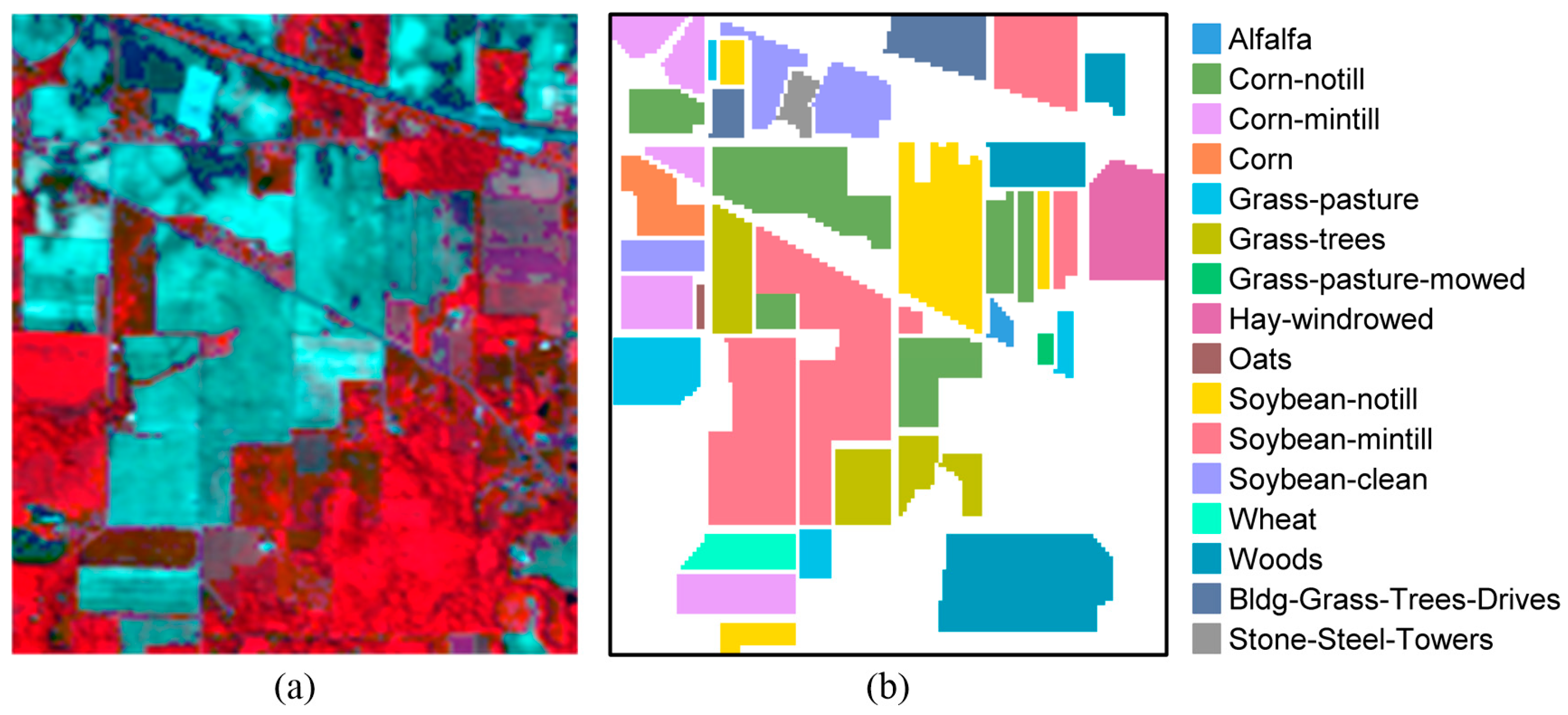
This data set was gathered by the Airborne Visible Infrared Imaging Spectrometer (AVIRIS) sensor over the agricultural regions in northwest Indiana’s Indian Pines test site. The spatial size of the data set is $145 \times 145$ pixels. Considering the effect of water absorption, 20 water absorption bands are removed, leaving 200 spectral bands for the HSI classification. The scene contains 16 land-cover classes. The detailed information of the ground-truth classes and the number of labeled samples are shown in

Table 1. Sixteen ground-truth classes of the Indian Pines data set.

Class	Name	Samples	Class	Name	Samples
1	Alfalfa	46	9	Oats	20
2	Corn-no till	1428	10	Soybean-no till	972
3	Corn-min till	830	11	Soybean-min till	2455
4	Corm	237	12	Soybean-clean	593
5	Grass/Pasture	483	13	Wheat	205
6	Grass/Trees	730	14	Woods	1265
7	Grass-pasture-mowed	28	15	Bldg-grass-tree-drives	386
8	Hay-windrowed	478	16	Stone-steel-towers	93

. The false-color composite image and the corresponding ground-truth map are shown in Figure 2. As the small size samples situation is mainly concerned in our work, ten samples from each class are randomly picked up to constitute the dictionary, and the remaining samples are used for testing.

4.1.2. University of Pavia Data Set

This data set was acquired by the Reflective Optics System Imaging Spectrometer (ROSIS) sensor over the urban area of the University of Pavia, Northern Italy. The original data set contains $610 \times 340$ pixels and 115 spectral bands, with 103 spectral bands reserved for analysis after removing 12 noisy bands. The nine ground-truth classes and the number of labeled samples from each class are listed in

Table 2. Nine ground-truth classes of the Pavia University data set.

Class	Name	Samples	Class	Name	Samples
1	Asphalt	6631	6	Bare soil	5029
2	Meadow	18649	7	Bitumen	1330
3	Gravel	2099	8	Self-Blocking Bricks	3682
4	Trees	3064	9	Shadows	947
5	Painted metal sheets	1345	/	/	/

. Figure 3 displays the false color image and the ground truth map. As for the number of training and testing samples, we randomly pick up ten labeled samples from each class for training and the rest for testing.

4.1.3. Salinas Data Set

This data set was also collected by the AVIRIS sensor over the area of Salinas Valley, CA, USA. The data contains $512 \times 217$ pixels and 224 spectral bands. Like the Indian Pines data set, we also remove 20 water absorption spectral bands and keep 204 spectral bands preserved for the HSI classification. The thorough description of labeled samples from the 16 ground-truth classes is provided in

Table 3. Sixteen ground-truth classes of the Salinas data set.

Class	Name	Samples	Class	Name	Samples
1	Broccoli green weeds 1	2009	9	Soil vinyard develop	6203
2	Broccoli green weeds 2	3726	10	Corn senesced weeds	3278
3	Fallow	1976	11	Lettuce romaine 4wk	1068
4	Fallow rough plow	1394	12	Lettuce romaine 5wk	1927
5	Fallow smooth	2678	13	Lettuce romaine 6wk	916
6	Stubble	3959	14	Lettuce romaine 7wk	1070
7	Celery	3579	15	Vinyard untrained	7268
8	Grapes untrained	11271	16	Vinyard vertical trellis	1807

. The false-color image and the corresponding ground-truth map are shown in Figure 4. Likewise, ten labeled samples from each class are chosen at random as the training dictionary and the remaining samples as the testing set.

4.2. Experimental Setting

4.2.1. Feature Extraction

For the proposed multi-feature-based representation methods, four features need to be extracted from the hyperspectral data, respectively. As described in Section 2.1, the Gabor texture feature, LBP feature and DMP shape feature are extracted from the first three principal components of the HSIs by using the principal component analysis. The detailed parameter values used in our work for the four feature descriptors are listed in

Table 4. Parameter setting for multiple feature descriptors.

Features	Parameters	Dimension
Spectral	All the bands of HSI	No. of bands
Gabor	Base image: PC1, PC2, PC3	180
	Scale: 1, 2, 3, 4, 5, 6, 7, 8, 9, 10
	Direction: 30°, 60°, 90°, 120°, 150°, 180°
DMP	Base image: PC1, PC2, PC3	48
	Size of SEs: 1, 4, 7, 10, 13, 16, 19, 22, 25
	No. of openings and closings: 8
LBP	Base image: PC1, PC2, PC3	177
	Local patch size: 21 × 21
	No. of neighbors and radius: (8, 1)

.

4.2.2. Parameter Tuning

The impact of the two regularization parameters λ and β on the classification performance of the proposed algorithms with the three hyperspectral data sets need to be investigated. The range of the parameter λ in the proposed MFCARC and MFCART algorithms is set as “${10}^{-8}, {10}^{-7}, {10}^{-6}, {10}^{-5}, {10}^{-4}, {10}^{-3}, {10}^{-2}, {10}^{-1}$”. For the parameter β in the MFCART, the candidate set is set as “${10}^{-5}, {10}^{-4}, {10}^{-3}, {10}^{-2},{10}^{-1},$1, 5, 10”. Considering that the value of the parameter λ involved in the single-feature-based CARC methods (i.e., CARC-Spectral, CARC-Gabor, CARC-DMP, and CARC-LBP) has great influence on the performance of the proposed multi-feature based representation methods, we examine the effect of λ on the performance of the CARC with four features, respectively. The overall accuracy tendencies of the single-feature-based CARC methods versus varying λ with three data sets are illustrated in Figure 5. As observed, the overall accuracies of the single-feature-based CARC methods generally increase significantly with the growing λ and then begin to decrease after the maximum value.

The influence of the regularization parameter β on the classification performance of the MFCART algorithm is also evaluated with all three data sets. As illustrated in Figure 6, the single-feature-based CART methods generally achieve better performance when the parameter β ranges from ${10}^{-5}$ to ${10}^{-1}$ except for the CART-spectral, as the CART-spectral achieves the best performance when β = 5 on the Indian Pines data set. The optimal parameter values of λ and β for the proposed MFCARC and MFCART algorithms on the three data sets are summarized in

Table 5. Optimal parameters for the proposed methods.

			Indian Pines	Pavia University	Salinas
MFCARC /MFCART	λ	Spectral	${10}^{-4}$	${10}^{-3}$	${10}^{-4}$
		Gabor	${10}^{-3}$	${10}^{-2}$	${10}^{-2}$
		DMP	${10}^{-3}$	${10}^{-2}$	${10}^{-3}$
		LBP	${10}^{-3}$	${10}^{-2}$	${10}^{-2}$
MFCART	β	Spectral	5	${10}^{-2}$	${10}^{-2}$
		Gabor	${10}^{-2}$	${10}^{-1}$	${10}^{-1}$
		DMP	${10}^{-1}$	${10}^{-2}$	${10}^{-2}$
		LBP	${10}^{-2}$	${10}^{-2}$	${10}^{-2}$

.

4.3. Classification Results

First, classification performance of the proposed CARC with the four features, i.e., CARC-Spectral, CARC-Gabor, CARC-DMP, and CARC-LBP is compared with the performance of the proposed MFCARC and MFCART, as shown in

Table 6. Classification accuracy (%) of the proposed CARC and CART with different single features and multiple features for the Salinas Data.

Method	CARC-Spectral	CARC-Gabor	CARC-DMP	CARC-LBP	MFCARC	MFCART
Broccoli green weeds 1	99.9 ± 0.22	84.4 ± 4.79	100 ± 0	100 ± 0	100 ± 0	100 ± 0
Broccoli green weeds 2	91.08 ± 5.04	79.14 ± 3.32	99.41 ± 0.35	95.32 ± 1.98	99.78 ± 0.35	99.78 ± 0.35
Fallow	62.44 ± 7.67	80.1 ± 5.83	81.73 ± 9.93	98.88 ± 1.1	99.09 ± 0.83	98.68 ± 1.37
Fallow rough plow	98.12 ± 2.09	92.9 ± 9.51	99.57 ± 0.4	99.71 ± 0.4	99.71 ± 0.65	99.86 ± 0.32
Fallow smooth	97.08 ± 1.53	75.06 ± 13.77	97.53 ± 0.73	92.28 ± 5.1	97.08 ± 0.72	97.38 ± 0.75
Stubble	99.95 ± 0.11	82.84 ± 10.25	99.24 ± 0.36	96.91 ± 2.07	99.9 ± 0.23	99.95 ± 0.11
Celery	99.83 ± 0.15	72.61 ± 6.92	99.61 ± 0.15	90.08 ± 4.06	99.72 ± 0.2	99.89 ± 0.15
Grapes untrained	50.07 ± 28.81	37.92 ± 10.16	69.82 ± 9.94	77.48 ± 13.14	83.11 ± 3.84	82.84 ± 2.42
Soil vineyard develop	99.81 ± 0.35	75.64 ± 4.82	94.6 ± 3.44	79.03 ± 3.56	98.9 ± 0.9	99.48 ± 0.35
Corn senesced weeds	84.1 ± 6.09	65.87 ± 7.49	77.61 ± 5.61	94.98 ± 2.66	97.06 ± 2.62	97.61 ± 0.79
Lettuce romaine 4 weeks	94.15 ± 1.81	77.36 ± 11.88	97.17 ± 1.16	87.92 ± 5.48	98.49 ± 1.08	99.06 ± 0.94
Lettuce romaine 5 weeks	86.98 ± 5.4	52.5 ± 6.68	99.38 ± 0.86	95.1 ± 6.11	99.9 ± 0.23	100 ± 0
Lettuce romaine 6 weeks	94.29 ± 9.72	95.38 ± 5.1	93.63 ± 2.62	89.23 ± 2.38	98.24 ± 1.25	98.46 ± 1.25
Lettuce romaine 7 weeks	92.83 ± 2.55	76.98 ± 2.55	96.23 ± 2.21	88.11 ± 5.36	99.25 ± 0.79	98.11 ± 2.31
Vineyard untrained	65.67 ± 16.85	42.98 ± 7.4	66.61 ± 7.75	83.42 ± 6.57	82.78 ± 6.35	88.02 ± 3.39
Vineyard vertical trellis	97 ± 1.87	46.11 ± 10.38	84.56 ± 10.32	94.67 ± 3.94	96.56 ± 5.63	96.78 ± 4.07
OA(%)	80.87 ± 4.02	62.84 ± 1.06	85.55 ± 1.99	87.73 ± 2.32	93.44 ± 0.5	94.21 ± 0.21
AA(%)	88.33 ± 1.3	71.11 ± 0.93	91.04 ± 1.2	91.45 ± 0.79	96.85 ± 0.35	97.24 ± 0.25
Kappa(%)	78.83 ± 4.33	59.53 ± 1.09	83.98 ± 2.17	86.42 ± 2.53	92.71 ± 0.55	93.57 ± 0.23

. The experiments of the proposed methods are conducted under the optimal parameters listed in Table 5. For the Salinas data set, ten labeled samples from each class are chosen at random for training and the rest for testing. It is observed that the proposed MFCARC and MFCART outperform the single-feature-based CARC methods, which demonstrates the effectiveness of combining multiple complementary features in the multi-task representation model. Besides, among those features, DMP and LBP features have superior performance and stronger class separability.

Subsequently, we compare the classification performance of the proposed MFCARC and MFCART methods with KSRC, MASR, CRT, KFRC-CKIR, MF-SRC, MF-JSRC, and MFASR. To avoid any bias, we repeat all the experiments ten times and record the averaged classification results, including the mean and standard deviation of OA, AA, CA, and the kappa coefficient. Classification performance of the proposed methods and its competitors for the Indian Pines data set is listed in

Table 7. Classification accuracy (%) of different classifiers for the Indian Pines data set.

Class	Train	KSRC	MASR	CRT	KFRC-CKIR	MF-SRC	MF-JSRC	MFASR	MFCARC	MFCART
1	10	82.78 ± 11.77	99.44 ± 1.24	72.78 ± 11.85	98.33 ± 2.48	97.78 ± 1.24	96.11 ± 1.52	97.78 ± 1.24	100 ± 0	100 ± 0
2	10	40.3 ± 9.95	58.27 ± 3.99	33.44 ± 9.02	62.78 ± 7.51	45.85 ± 10.19	51.99 ± 3.54	65.26 ± 3.4	69.61 ± 9.48	72.65 ± 5.14
3	10	45.01 ± 8.55	68.51 ± 6.51	40.27 ± 5.91	86 ± 8.04	58.59 ± 6.56	65.1 ± 11.14	70.44 ± 11.73	75.93 ± 4.43	78.76 ± 3.07
4	10	58.02 ± 7.6	90.66 ± 5.53	40.35 ± 17.8	93.22 ± 9.63	72.86 ± 12.27	82.03 ± 7.29	91.01 ± 5.88	95.12 ± 5.07	98.52 ± 2.69
5	10	76.98 ± 7.19	86.22 ± 8.34	74.38 ± 9.24	88.75 ± 2.95	78.94 ± 8.05	84.4 ± 3	86.93 ± 4.82	82.73 ± 8.38	87.37 ± 3.33
6	10	83.86 ± 5.2	95.03 ± 2	82.83 ± 4.31	94.5 ± 5.83	81.97 ± 6.81	91.47 ± 1.1	91.31 ± 6.23	98.75 ± 2.43	97.22 ± 2.52
7	10	92.78 ± 5.27	100 ± 0	85.56 ± 4.97	100 ± 0	94.44 ± 0.13	100 ± 0	98.89 ± 2.48	100 ± 0	100 ± 0
8	10	83.1 ± 7.11	86.45 ± 11.01	65.68 ± 11.84	95.43 ± 7.47	97.05 ± 1.38	99.27 ± 0.89	99.91 ± 0.12	100 ± 0	100 ± 0
9	10	85 ± 9.72	100 ± 0	98 ± 4.47	100 ± 0	100 ± 0	100 ± 0	100 ± 0	100 ± 0	100 ± 0
10	10	46.5 ± 8.42	80.94 ± 9.56	35.05 ± 8.12	89.71 ± 2.86	55.72 ± 5.58	69.48 ± 3.63	81.6 ± 10.79	83.42 ± 1.95	83.33 ± 2.95
11	10	44.13 ± 8.34	68.28 ± 3.59	43.99 ± 7.83	73.88 ± 11.06	49.35 ± 3.77	58.17 ± 5.54	73.45 ± 4.56	83.48 ± 2.49	83.23 ± 4.37
12	10	43.98 ± 7.99	56.71 ± 11.94	34.13 ± 4.45	79.59 ± 9.54	70.98 ± 4.35	74.24 ± 4.66	86.42 ± 6.05	81.53 ± 9.53	92.45 ± 3.68
13	10	93.28 ± 4.79	99.69 ± 0.46	94.56 ± 2.6	97.95 ± 0.89	99.18 ± 0.46	99.69 ± 0.28	99.49 ± 0	99.49 ± 1.15	100 ± 0
14	10	76.08 ± 7.25	86.07 ± 4.84	69.39 ± 13.25	91.08 ± 7.84	89.37 ± 4.6	94.63 ± 4.54	95.31 ± 3.93	96.83 ± 2.48	98.8 ± 1.4
15	10	43.14 ± 6.41	67.13 ± 19.51	31.81 ± 7.62	88.03 ± 7.87	93.03 ± 1.58	98.03 ± 1.26	94.63 ± 5.38	97.61 ± 4.64	99.33 ± 1.12
16	10	88.92 ± 5.62	99.28 ± 0.66	92.05 ± 4.39	98.31 ± 1.83	99.04 ± 0.54	99.28 ± 0.66	98.07 ± 1.08	100 ± 0	100 ± 0
OA		55.9 ± 3.08	74.76 ± 2.15	50.21 ± 1.9	82.24 ± 1.24	66.2 ± 2.23	73.33 ± 2.19	81.48 ± 2.64	85.62 ± 1.69	87.35 ± 1.56
AA		67.74 ± 2.4	83.92 ± 2.36	62.14 ± 2.09	89.85 ± 1.76	80.26 ± 1.08	85.24 ± 1.06	89.41 ± 1.64	91.53 ± 1.36	93.23 ± 0.81
Kappa		50.63 ± 3.3	71.47 ± 2.43	44.35 ± 1.99	79.96 ± 1.39	62.19 ± 2.37	69.99 ± 2.4	79.03 ± 2.99	83.69 ± 1.87	85.66 ± 1.61

. From Table 7, it is observed that the proposed methods provide remarkable performance with approximately 20% higher improvement in terms of OA compared with the state-of-the-art KSRC, CRT, and MF-SRC. In addition, when compared with the multi-feature-based classification algorithms such as MF-SRC, MF-JSRC, and MFASR, our proposed methods show better performance. Besides, the classification maps generated by the proposed methods and other comparative methods are shown in Figure 7b–j. It shows that the proposed methods achieve promising performance in both large homogeneous regions and regions of small objects.

The detailed classification performance for the University of Pavia data set is given in

Table 8. Classification accuracy (%) of different classifiers for the University of Pavia data set.

Class	Train	KSRC	MASR	CRT	KFRC-CKIR	MF-SRC	MF-JSRC	MFASR	MFCARC	MFCART
1	10	55.91 ± 5.18	46.48 ± 12.31	35.79 ± 5.47	83 ± 6.99	80.73 ± 4.31	84.89 ± 6.04	94.4 ± 2.75	85.05 ± 4.01	88.47 ± 2.09
2	10	61.29 ± 9.04	71.56 ± 3.56	68.04 ± 6.28	80.75 ± 3.64	69.69 ± 7.48	67.9 ± 11.17	70.97 ± 6.82	86.95 ± 2.68	85.75 ± 2.19
3	10	72.03 ± 7.48	77.3 ± 7.51	67.57 ± 7.4	78.04 ± 4.79	81.53 ± 11.82	82.68 ± 11.85	96.37 ± 1.28	98.8 ± 0.79	99.12 ± 1.5
4	10	84.73 ± 5.43	95.43 ± 1.84	91.43 ± 6.46	91.66 ± 4.33	96.98 ± 1.53	97.18 ± 1.36	95.87 ± 0.58	99.45 ± 0.27	99.56 ± 0.61
5	10	99.61 ± 0.24	100 ± 0	99.73 ± 0.11	99.68 ± 0.15	100 ± 0	100 ± 0	99.9 ± 0.07	100 ± 0	100 ± 0
6	10	68.86 ± 7.67	57.78 ± 8.66	62.95 ± 11.1	77.4 ± 4.04	79.84 ± 12.31	85.62 ± 11.92	89.7 ± 4.52	92.03 ± 2.46	90.6 ± 2.28
7	10	76.83 ± 12.66	95.26 ± 4.07	69.91 ± 6.65	88.06 ± 7.62	100 ± 0	100 ± 0	99.86 ± 0.08	100 ± 0	100 ± 0
8	10	43.33 ± 6.58	86.61 ± 7.79	45.36 ± 10.36	77.28 ± 8.07	85.83 ± 4.94	88.66 ± 5.8	97.66 ± 1.16	96.14 ± 2.75	96.09 ± 3.8
9	10	79.21 ± 8.2	65.04 ± 4.95	80.96 ± 3.15	91.46 ± 3.96	98.94 ± 2.38	98.51 ± 3.33	99.06 ± 1.18	98.58 ± 1.6	98.4 ± 2.21
OA		64.07 ± 4.1	70.81 ± 3.07	63.47 ± 1.88	82.11 ± 2.02	79.04 ± 2.67	82.89 ± 4.74	84.54 ± 3.08	90.59 ± 2.87	90.44 ± 2.76
AA		71.31 ± 1.75	77.27 ± 1.75	69.08 ± 1.01	85.26 ± 1.5	88.17 ± 1.45	89.49 ± 1.84	93.75 ± 0.88	95.22 ± 0.4	95.33 ± 0.49
Kappa		55.38 ± 4.25	63.02 ± 3.69	54.16 ± 1.84	76.97 ± 2.47	73.82 ± 3.02	75.03 ± 5.42	80.63 ± 3.61	87.85 ± 2.92	87.68 ± 2.97

, and the classification maps are shown in Figure 8b‒j. The proposed methods achieve the best performance with the OA value reaching about 90%. There exists significant improvement when compared with multi-feature-based classification methods. Specifically, our methods produce nearly 11%, 8%, and 6% improvement in terms of OA compared with MF-SRC, MF-JSRC, and MFASR. As illustrated in Figure 8, our methods result in more accurate classification maps than other classifiers.

The classification performance for Salinas data set is listed in

Table 9. Classification accuracy (%) of different classifiers for the Salinas data set.

Class	Train	KSRC	MASR	CRT	KFRC-CKIR	MF-SRC	MF-JSRC	MFASR	MFCARC	MFCART
1	10	98.84 ± 0.85	99.97 ± 0.07	98.41 ± 1.24	99.84 ± 0.24	98.8 ± 1.25	98.6 ± 3.13	99.97 ± 0.04	100 ± 0	100 ± 0
2	10	98.1 ± 0.99	99.3 ± 0.45	99.6 ± 0.3	99.64 ± 0.16	94.3 ± 4.9	96.67 ± 1.62	99 ± 0.79	99.78 ± 0.35	99.78 ± 0.35
3	10	85.11 ± 5.31	96.06 ± 7.52	86.2 ± 6.47	99.93 ± 0.17	95.13 ± 0.28	91.57 ± 9.09	98.1 ± 2.35	99.09 ± 0.83	98.68 ± 1.37
4	10	98.24 ± 1.88	97.9 ± 1.17	92.14 ± 6.47	99.13 ± 0.53	97.39 ± 4.24	99.86 ± 0.32	99.84 ± 0.08	99.71 ± 0.65	99.86 ± 0.32
5	10	93.96 ± 6.44	97.09 ± 3.2	89.03 ± 7.14	98.84 ± 0.52	97.45 ± 1.62	97.08 ± 2.02	98.75 ± 0.38	97.08 ± 0.72	97.38 ± 0.75
6	10	99.58 ± 0.19	99.98 ± 0.01	99.84 ± 0.05	99.84 ± 0.01	99.8 ± 0.33	100 ± 0	99.64 ± 0.17	99.9 ± 0.23	99.95 ± 0.11
7	10	99.32 ± 0.14	99.98 ± 0.01	99.66 ± 0.1	99.32 ± 0.54	95.35 ± 2.72	97.2 ± 3.21	99.42 ± 0.18	99.72 ± 0.2	99.89 ± 0.15
8	10	60.73 ± 10.73	64.09 ± 10.87	65.52 ± 7.38	75.74 ± 5	61.19 ± 5.49	78.47 ± 7.29	77.33 ± 6.41	83.11 ± 3.84	82.84 ± 2.42
9	10	97.6 ± 0.24	99.21 ± 0.42	98.75 ± 1.66	99.85 ± 0.21	97 ± 2.08	98.55 ± 1.16	99.58 ± 0.18	98.9 ± 0.9	99.48 ± 0.35
10	10	86.38 ± 6.33	92.5 ± 5.31	83.12 ± 7.54	92.42 ± 2.64	88.56 ± 4.07	88.2 ± 7.13	94.8 ± 1.62	97.06 ± 2.62	97.61 ± 0.79
11	10	92.99 ± 4.21	99.77 ± 0.27	94.91 ± 1.29	98.04 ± 2.02	95.66 ± 1.08	99.43 ± 0.84	97.81 ± 1.55	98.49 ± 1.08	99.06 ± 0.94
12	10	99.73 ± 0.54	99.91 ± 0.07	85.55 ± 3.2	100 ± 0	100 ± 0	99.9 ± 0.23	100 ± 0	99.9 ± 0.23	100 ± 0
13	10	97.72 ± 0.64	99.29 ± 1.03	98.23 ± 0.92	99.21 ± 0.57	95.16 ± 1.84	97.14 ± 2.28	97.64 ± 0.57	98.24 ± 1.25	98.46 ± 1.25
14	10	94.12 ± 2.09	98.3 ± 0.6	92.81 ± 1.81	96.93 ± 1.54	94.53 ± 3.09	97.74 ± 1.43	94.77 ± 2.55	99.25 ± 0.79	98.11 ± 2.31
15	10	61.47 ± 9.94	72 ± 11.61	58.44 ± 6.05	87.79 ± 4.44	71.46 ± 5.21	74.52 ± 4.86	76.52 ± 11.24	82.78 ± 6.35	88.02 ± 3.39
16	10	94.97 ± 4.68	97.22 ± 3.95	93.76 ± 3.87	94.28 ± 5.07	86.78 ± 4.52	89.67 ± 2.03	93.52 ± 4.47	96.56 ± 5.63	96.78 ± 4.07
OA		83.92 ± 1.27	87.66 ± 0.92	83.69 ± 1.39	92.35 ± 0.92	85.19 ± 0.68	89.83 ± 1.76	91.08 ± 0.34	93.44 ± 0.5	94.21 ± 0.21
AA		91.18 ± 0.69	94.54 ± 0.8	89.75 ± 0.7	96.3 ± 0.35	91.78 ± 0.48	94.04 ± 1.01	95.42 ± 0.29	96.85 ± 0.35	97.24 ± 0.25
Kappa		82.16 ± 1.38	86.3 ± 1.01	81.87 ± 1.52	91.51 ± 1.02	83.59 ± 0.74	88.69 ± 1.95	90.08 ± 0.39	92.71 ± 0.55	93.57 ± 0.23

, and the classification maps generated by different classifiers are shown in Figure 9b–j. From Table 9, it is seen that the proposed MFCARC and MFCART methods outperform other comparative algorithms. For the Salinas data, there are two classes that are very difficult to be distinguished, i.e., class 8 (Grapes untrained) and class 15 (Vinyard untrained). This is because these two classes are not only spatially adjacent, but also have very similar spectral reflectance curves. From the classification maps, we can see that our proposed methods produce satisfactory results. The accuracy for class 15 of MFCART improves nearly 6% compared with MFCARC, which validates the effectiveness of the MFCART.

To further validate the effectiveness of the proposed methods, we compare our methods with several recent deep-learning-based classifiers. The experimental results over the Indian Pines data set and the University of Paiva data set are reported in

Table 10. Classification performance of different methods over the Indian Pines data set.

Class	Train	2-D CNN	3-D CNN	GFELM-AE	SSCL2DNN	SSCL3DNN	MFCARC	MFCART
1	10	94.44	97.22	79.13	98.15	100.00	100.00	100.00
2	10	37.83	53.60	50.98	38.65	53.30	69.61	72.65
3	10	47.59	61.78	52.76	46.34	50.37	75.93	78.76
4	10	76.12	96.83	45.21	79.88	88.63	95.12	98.52
5	10	58.01	75.90	61.50	61.95	76.58	82.73	87.37
6	10	46.06	78.47	82.09	65.56	90.17	98.75	97.22
7	10	100.00	100.00	84.62	100.00	100.00	100.00	100.00
8	10	93.33	99.83	75.60	94.59	100.00	100.00	100.00
9	10	100.00	100.00	68.57	100.00	100.00	100.00	100.00
10	10	47.80	63.56	63.81	66.22	75.36	83.42	83.33
11	10	42.45	55.09	69.70	50.46	59.66	83.48	83.23
12	10	45.97	67.03	44.72	60.83	64.97	81.53	92.45
13	10	86.97	96.82	84.81	96.58	99.79	99.49	100.00
14	10	69.94	88.11	61.89	73.86	88.29	96.83	98.80
15	10	69.95	84.20	32.70	84.13	87.66	97.61	99.33
16	10	90.60	98.31	89.64	91.16	100.00	100.00	100.00
OA		53.08	69.21	61.42	60.59	71.28	85.62	87.35
AA		69.19	82.30	65.48	75.52	83.42	91.53	93.23
Kappa		47.72	65.56	55.26	56.12	67.83	83.69	85.66

and

Table 11. Classification performance of different methods over the University of Paiva data set.

Class	Train	2-D CNN	3-D CNN	GFELM-AE	SSCL2DNN	SSCL3DNN	MFCARC	MFCART
1	10	37.14	42.58	31.25	49.43	69.89	85.05	88.47
2	10	43.51	84.89	72.04	76.89	82.44	86.95	85.75
3	10	34.96	25.50	39.23	39.38	65.10	98.80	99.12
4	10	59.74	34.01	67.63	62.48	90.48	99.45	99.56
5	10	75.18	91.41	71.47	84.42	94.83	100.00	100.00
6	10	23.30	37.47	46.62	41.29	82.37	92.03	90.60
7	10	35.86	80.61	30.08	61.16	89.32	100.00	100.00
8	10	63.47	10.74	53.02	66.68	84.71	96.14	96.09
9	10	86.27	21.10	34.20	83.46	86.91	98.58	98.40
OA		44.30	58.50	47.16	64.59	81.11	90.59	90.44
AA		51.05	47.59	49.50	62.80	82.90	95.22	95.33
Kappa		32.59	44.68	36.42	54.45	75.65	87.85	87.68

. From Table 10 and Table 11, it is observed that the proposed methods outperform deep-learning-based models on both data sets. Specifically, compared with the state-of-the-art GFELM-AE, SSCL2DNN and SSCL3DNN algorithms, MFCART obtains 25.93%, 26.76%, and 16.07% gains in OA on the Indian Pines data set. For the University of Pavia data set, the proposed MFCARC yields an accuracy of 90.59%, achieving 46.29%, 32.09%, and 9.48% improvement over the 2-D CNN, 3-D CNN, and SSCL3DNN methods, respectively. Based on the experimental results, it demonstrates the effectiveness and the superiority of the proposed MFCARC and MFCART methods.

5. Discussion

5.1. Coefficients Distribution

To validate the effectiveness of the proposed MFCARC and MFCART algorithms, the representation coefficients distribution on training samples and the corresponding reconstruction residuals in MFCARC and MFCART are displayed in Figure 10, Figure 11, Figure 12 and Figure 13. Specifically, 10 training samples from each class are randomly chosen to construct the training dictionary and a sample belonging to class 6 (i.e., grass/trees) from the Indian Pines data set is selected as the test sample. As illustrated in Figure 1, for the four features, the representation coefficients distribution presents such a characteristic that higher weights are concentrated in the class to which the test sample belongs. However, the representation coefficients obtained by the Gabor feature make a wrong prediction by classifying the test sample to class 4, as shown in Figure 11b. Figure 12b illustrates the representation coefficients distribution obtained by the MFCART using the four features. As can be observed, the largest weight coefficients are distributed in the class of the test sample, with the highest coefficients being much higher than that of MFCARC. Besides, the weight coefficients distributed in the remaining classes are much smaller or even zero, this characteristic is particularly prominent on the coefficients obtained by the Spectral feature. Therefore, such a coefficient distribution is quite close to the distribution of the ideal representation model that we mentioned earlier. It can be clearly seen from Figure 13 that the representation coefficients obtained by the MFCART with the four features can make correct prediction by classifying the test sample to the right class. By comparing Figure 11 and Figure 13, it is seen that the test sample that was previously misclassified by the MFCARC with Gabor feature is now corrected by the MFCART with Gabor feature. This demonstrates the effectiveness and superiority of the MFCART by taking the correlation between the test sample and the training samples into consideration.

5.2. Influence of Dictionary Size

Figure 14a–c shows the influence of the training dictionary size on the OA and the kappa coefficient for the Indian Pines, University of Pavia, and Salinas data sets. The candidate set for the number of training samples per class is set as $\left\{5, 10, 15, 20, 25, 30\right\}.$ From Figure 14, it is observed that the dictionary size has a decisive influence on the classification performance of the proposed MFCARC and MFCART methods. Specifically, when the training dictionary has a small number of samples, the classification performance is not so satisfactory for the Indian Pines data set. The main reason is that the information covered by the dictionary is insufficient to reflect the precise correlation structure of the dictionary. When the size of the training dictionary becomes larger, the overall classification accuracy and the kappa coefficient of the two proposed methods increase on all three data sets.

5.3. Computing Time

In order to evaluate the computational complexity of the various classification algorithms, all experiments are implemented using MATLAB on a 2.60 GHz CPU workstation with 16 GB of RAM. More detailed information is summarized and then listed in

Table 12. Execution time (in seconds) for the classification of the Indian Pines data set.

Method	KSRC	MASR	CRT
Time	34.51	82.25	9.61
Method	KFRC-CKIR	MF-SRC	MF-JSRC
Time	11.62	7.15	15.32
Method	MFASR	MFCARC	MFCART
Time	66.2	611.73	671.54

. As illustrated in Table 12, CRT and MF-SRC are the two fastest algorithms among all these classifiers, with running time less than ten seconds. In comparison, the running time of our proposed algorithms is much slower due to the iterative process involved in the optimization algorithms. Specifically, for the proposed MFCARC and MFCART methods, the dominant computational cost comes from the learning of representation coefficients via the correlation regularization problem in multiple-feature-based subspace, which is implemented by the Iteratively Reweighted Least Squares (IRLS) method. As shown in Table 12, although MFCART costs more time than MFCARC owing to the integration of the distance-weighted Tikhonov regularization, MFCART achieves higher classification accuracy. On the other hand, both of the proposed algorithms provide better classification performance under the small size samples situations, compared with other state-of-the-art classifiers.

6. Conclusions

In this paper, a new representation-based classifier CARC is proposed to perform sample selection and group correlated samples simultaneously. Owing to the adaptive property of the regularization, CARC is capable of balancing between SRC and CRC adaptively according to the precise correlation structure of the dictionary, which overcomes the intrinsic limitations of the traditional SR- and CR-based classification methods in HSI classification. In addition, by taking the correlation between the test sample and the training samples into consideration, CART is developed to make the representation model reveal the true geometry of feature space. Moreover, aiming at solving the small training samples issue, multi-feature representation frameworks are constructed according to the proposed CARC and CART, leading to MFCARC and MFCART frameworks, which can build more accurate representation models for hyperspectral data under the small size samples situations. Experimental results show that the MFCARC and MFCART achieve superior performance than state-of-the-art algorithms.

However, there also exist certain limitations for the proposed methods. In our proposed methods, training samples are directly used as training atoms of the dictionary and the random sampling strategy is adopted for constructing the dictionary. Considering that constructing a compact and representative dictionary is beneficial for the sample representation, our future research will focus on the design of the discriminative dictionary and the integration of the dictionary learning process to further improve the classification performance under the small size samples situations.

References

1. Zhang, N.; Yang, G.; Pan, Y.; Yang, X.; Chen, L.; Zhao, C. A review of advanced technologies and development for hyperspectral-based plant disease detection in the past three decades. Remote Sens. 2020, 12, 3188. [Google Scholar] [CrossRef]
2. Lv, M.; Fowler, J.E.; Jing, L. Spatial functional data analysis for the spatial-spectral classification of hyperspectral imagery. IEEE Geosci. Remote Sens. Lett. 2018, 16, 1–5. [Google Scholar] [CrossRef]
3. Liu, N.; Li, W.; Tao, R.; Fowler, J.E. Wavelet-domain low-rank/group-sparse destriping for hyperspectral imagery. IEEE Trans. Geosci. Remote Sens. 2019, 57, 10310–10321. [Google Scholar] [CrossRef]
4. Huang, H.; Chen, M.; Duan, Y. Dimensionality reduction of hyperspectral image using spatial-spectral regularized sparse hypergraph embedding. Remote Sens. 2019, 11, 1039. [Google Scholar] [CrossRef] [Green Version]
5. Hennessy, A.; Clarke, K.; Lewis, M. Hyperspectral classification of plants: A review of waveband selection generalisability. Remote Sens. 2020, 12, 113. [Google Scholar] [CrossRef] [Green Version]
6. Ghamisi, P.; Maggiori, E.; Li, S.; Souza, R.; Tarablaka, Y.; Moser, G.; De Giorgi, A.; Fang, L.; Chen, Y.; Chi, M.; et al. New frontiers in spectral-spatial hyperspectral image classification: The latest advances based on mathematical morphology, Markov random fields, segmentation, sparse representation, and deep learning. IEEE Geosci. Remote Sens. Mag. 2018, 6, 10–43. [Google Scholar] [CrossRef]
7. Audebert, N.; Le Saux, B.; Lefèvre, S. Deep learning for classification of hyperspectral data: A comparative review. IEEE Geosci. Remote Sens. Mag. 2019, 7, 159–173. [Google Scholar] [CrossRef] [Green Version]
8. Li, S.; Song, W.; Fang, L.; Chen, Y.; Ghamisi, P.; Benediktsson, J.A. Deep learning for hyperspectral image classification: An overview. IEEE Trans. Geosci. Remote Sens. 2019, 57, 6690–6709. [Google Scholar] [CrossRef] [Green Version]
9. Wright, J.; Yang, A.Y.; Ganesh, A.; Sastry, S.S.; Ma, Y. Robust face recognition via space representation. IEEE Trans. Pattern Anal. Mach. Intell. 2009, 31, 210–227. [Google Scholar] [CrossRef] [PubMed] [Green Version]
10. Chen, Y.; Nasrabadi, N.M.; Tran, T.D. Hyperspectral image classification using dictionary-based sparse representation. IEEE Trans. Geosci. Remote Sens. 2011, 49, 3973–3985. [Google Scholar] [CrossRef]
11. Zhang, H.; Li, J.; Huang, Y.; Zhang, L. A nonlocal weighted joint sparse representation classification method for hyperspectral imagery. IEEE J. Sel. Top. Appl. Earth Obs. Remote Sens. 2014, 7, 2056–2065. [Google Scholar] [CrossRef]
12. Hu, S.; Peng, J.; Fu, Y.; Li, L. Kernel joint sparse representation based on self-paced learning for hyperspectral image classification. Remote Sens. 2019, 11, 1114. [Google Scholar] [CrossRef] [Green Version]
13. Li, C.; Ma, Y.; Mei, X.; Liu, C.; Ma, J. Hyperspectral image classification with robust sparse representation. IEEE Geosci. Remote Sens. Lett. 2016, 13, 641–645. [Google Scholar] [CrossRef]
14. Zhang, X.; Song, Q.; Gao, Z.; Zheng, Y.; Weng, P.; Jiao, L.C. Spectral-spatial feature learning using cluster-based group sparse coding for hyperspectral image classification. IEEE J. Sel. Top. Appl. Earth Obs. Remote Sens. 2016, 9, 4142–4159. [Google Scholar] [CrossRef]
15. Yu, H.; Gao, L.; Liao, W.; Zhang, B. Group sparse representation based on nonlocal spatial and local spectral similarity for hyperspectral imagery classification. Sensors 2018, 18, 1695. [Google Scholar] [CrossRef] [PubMed] [Green Version]
16. Zhang, L.; Yang, M.; Feng, X. Sparse representation or collaborative representation: Which helps face recognition? In Proceedings of the 2011 International Conference on Computer Vision, Institute of Electrical and Electronics Engineers, Barcelona, Spain, 3–6 November 2011; pp. 471–478. [Google Scholar]
17. Fan, Z.; Ni, M.; Zhu, Q.; Liu, E. Weighted sparse representation for face recognition. Neurocomputing 2015, 151, 304–309. [Google Scholar] [CrossRef]
18. Li, W.; Tramel, E.W.; Prasad, S.; Fowler, J.E. Nearest regularized subspace for hyperspectral classification. IEEE Trans. Geosci. Remote Sens. 2014, 52, 477–489. [Google Scholar] [CrossRef] [Green Version]
19. Li, W.; Du, Q.; Xiong, M. Kernel collaborative representation with tikhonov regularization for hyperspectral image classification. IEEE Geosci. Remote Sens. Lett. 2014, 12, 1–5. [Google Scholar] [CrossRef]
20. Du, P.; Gan, L.; Xia, J.; Wang, D. Multikernel adaptive collaborative representation for hyperspectral image classification. IEEE Trans. Geosci. Remote Sens. 2018, 56, 4664–4677. [Google Scholar] [CrossRef]
21. Li, W.; Zhang, Y.; Liu, N.; Du, Q.; Tao, R. Structure-aware collaborative representation for hyperspectral image classification. IEEE Trans. Geosci. Remote Sens. 2019, 57, 7246–7261. [Google Scholar] [CrossRef]
22. Tu, B.; Zhou, C.; Liao, X.; Zhang, G.; Peng, Y. Spectral-spatial hyperspectral classification via structural-kernel collaborative representation. IEEE Geosci. Remote Sens. Lett. 2020, 1–5. [Google Scholar] [CrossRef]
23. Iordache, M.-D.; Bioucas-Dias, J.M.; Plaza, A. Sparse unmixing of hyperspectral data. IEEE Trans. Geosci. Remote Sens. 2011, 49, 2014–2039. [Google Scholar] [CrossRef] [Green Version]
24. Zou, H.; Hastie, T. Regularization and variable selection via the elastic net. J. R. Stat. Soc. Ser. B 2005, 67, 301–320. [Google Scholar] [CrossRef] [Green Version]
25. Li, W.; Du, Q.; Zhang, F.; Hu, W. Hyperspectral image classification by fusing collaborative and sparse representations. IEEE J. Sel. Top. Appl. Earth Obs. Remote Sens. 2016, 9, 4178–4187. [Google Scholar] [CrossRef]
26. Gan, L.; Du, P.; Xia, J.; Meng, Y. Kernel fused representation-based classifier for hyperspectral imagery. IEEE Geosci. Remote Sens. Lett. 2017, 14, 684–688. [Google Scholar] [CrossRef]
27. Liu, G.; Qi, L.; Tie, Y.; Ma, L. Hyperspectral image classification using kernel fused representation via a spatial-spectral composite kernel with ideal regularization. IEEE Geosci. Remote Sens. Lett. 2019, 16, 1422–1426. [Google Scholar] [CrossRef]
28. Bian, X.; Chen, C.; Xu, Y.; Du, Q. Robust hyperspectral image classification by multi-layer spatial-spectral sparse representations. Remote Sens. 2016, 8, 985. [Google Scholar] [CrossRef] [Green Version]
29. Soomro, B.N.; Xiao, L.; Huang, L.; Soomro, S.H.; Molaei, M. Bilayer elastic net regression model for supervised spectral-spatial hyperspectral image classification. IEEE J. Sel. Top. Appl. Earth Obs. Remote Sens. 2016, 9, 4102–4116. [Google Scholar] [CrossRef]
30. Soomro, B.N.; Xiao, L.; Molaei, M.; Huang, L.; Lian, Z.; Soomro, S.H. Local and nonlocal context-aware elastic net representation-based classification for hyperspectral images. IEEE J. Sel. Top. Appl. Earth Obs. Remote Sens. 2017, 10, 2922–2939. [Google Scholar] [CrossRef]
31. Gao, L.; Qi, L.; Chen, E.; Guan, L. Discriminative multiple canonical correlation analysis for information fusion. IEEE Trans. Image Process. 2018, 27, 1951–1965. [Google Scholar] [CrossRef] [PubMed]
32. Gao, L.; Zhang, R.; Qi, L.; Chen, E.; Guan, L. The labeled multiple canonical correlation analysis for information fusion. IEEE Trans. Multimed. 2019, 21, 375–387. [Google Scholar] [CrossRef]
33. Su, H.; Zhao, B.; Du, Q.; Du, P.; Xue, Z. Multifeature dictionary learning for collaborative representation classification of hyperspectral imagery. IEEE Trans. Geosci. Remote Sens. 2018, 56, 2467–2484. [Google Scholar] [CrossRef]
34. Zhang, E.; Zhang, X.; Liu, H.; Jiao, L. Fast multifeature joint sparse representation for hyperspectral image classification. IEEE Geosci. Remote Sens. Lett. 2015, 12, 1397–1401. [Google Scholar] [CrossRef]
35. Jia, S.; Hu, J.; Xie, Y.; Shen, L.; Jia, X.; Li, Q. Gabor cube selection based multitask joint sparse representation for hyperspectral image classification. IEEE Trans. Geosci. Remote Sens. 2016, 54, 3174–3187. [Google Scholar] [CrossRef]
36. Fang, L.; Wang, C.; Li, S.; Benediktsson, J.A. Hyperspectral image classification via multiple-feature-based adaptive sparse representation. IEEE Trans. Instrum. Meas. 2017, 66, 1646–1657. [Google Scholar] [CrossRef]
37. He, Z.; Li, J.; Liu, L.; Liu, K.; Zhuo, L. Fast three-dimensional empirical mode decomposition of hyperspectral images for class-oriented multitask learning. IEEE Trans. Geosci. Remote Sens. 2016, 54, 6625–6643. [Google Scholar] [CrossRef]
38. He, Z.; Wang, Y.; Hu, J. Joint sparse and low-rank multitask learning with laplacian-like regularization for hyperspectral classification. Remote Sens. 2018, 10, 322. [Google Scholar] [CrossRef] [Green Version]
39. Gan, L.; Xia, J.; Du, P.; Chanussot, J. Multiple feature kernel sparse representation classifier for hyperspectral imagery. IEEE Trans. Geosci. Remote Sens. 2018, 56, 5343–5356. [Google Scholar] [CrossRef]
40. Li, W.; Du, Q. Gabor-filtering-based nearest regularized subspace for hyperspectral image classification. IEEE J. Sel. Top. Appl. Earth Obs. Remote Sens. 2014, 7, 1012–1022. [Google Scholar] [CrossRef]
41. Jia, S.; Shen, L.; Li, Q. Gabor feature-based collaborative representation for hyperspectral imagery classification. IEEE Trans. Geosci. Remote Sens. 2015, 53, 1118–1129. [Google Scholar] [CrossRef]
42. Lv, Z.Y.; Zhang, P.; Benediktsson, J.A.; Shi, W.Z. Morphological profiles based on differently shaped structuring elements for classification of images with very high spatial resolution. IEEE J. Sel. Top. Appl. Earth Obs. Remote Sens. 2014, 7, 4644–4652. [Google Scholar] [CrossRef]
43. Li, W.; Chen, C.; Su, H.; Du, Q. Local binary patterns and extreme learning machine for hyperspectral imagery classification. IEEE Trans. Geosci. Remote Sens. 2015, 53, 3681–3693. [Google Scholar] [CrossRef]
44. Becker, S.; Bobin, J.; Candès, E.J. NESTA: A fast and accurate first-order method for sparse recovery. SIAM J. Imaging Sci. 2011, 4, 1–39. [Google Scholar] [CrossRef] [Green Version]
45. Yang, J.; Zhang, Y. Alternating direction algorithms for 1 - problems in compressive sensing. SIAM J. Sci. Comput. 2011, 33, 250–278. [Google Scholar] [CrossRef]
46. Grave, E.; Obozinski, G.R.; Bach, F.R. Trace lasso: A trace norm regularization for correlated designs. Adv. Neural Inf. Process. Syst. 2011, arXiv:1109.1990v1. [Google Scholar]
47. Lin, Z.; Chen, M.; Ma, Y. The Augmented Lagrange Multiplier Method for Exact Recovery of a Corrupted Low-Rank Matrices; UIUC Tech. Rep. UILU-ENG-09-2215; Department of Electrical and Computer Engineering UIUC: Champaign, IL, USA, 2009. [Google Scholar]
48. Lu, C.; Lin, Z.; Yan, S. Smoothed low rank and sparse matrix recovery by iteratively reweighted least squares minimization. IEEE Trans. Image Process. 2015, 24, 646–654. [Google Scholar] [CrossRef] [PubMed] [Green Version]
49. Daubechies, I.; Devore, R.; Fornasier, M.; Güntürk, C.S. Iteratively reweighted least squares minimization for sparse recovery. Commun. Pure Appl. Math. 2010, 63, 1–38. [Google Scholar] [CrossRef] [Green Version]
50. Mohan, K.; Fazel, M. Iterative reweighted algorithms for matrix rank minimization. J. Mach. Learn. Res. 2012, 13, 3441–3473. [Google Scholar]
51. Argyriou, A.; Evgeniou, T.; Pontil, M. Multi-task feature learning. Adv. Neural Inf. Process. Syst. 2007. [Google Scholar] [CrossRef]
52. Bach, F.; Jenatton, R.; Mairal, J.; Obozinski, G. Optimization with sparsity-inducing penalties. Found. Trends. Mach. Learn. 2011, 4, 1–106. [Google Scholar] [CrossRef]
53. Argyriou, A.; Evgeniou, T.; Pontil, M. Convex multi-task feature learning. Mach. Learn. 2008, 73, 243–272. [Google Scholar] [CrossRef] [Green Version]
54. Zhang, L.; Zhou, W.-D.; Chang, P.-C.; Liu, J.; Yan, Z.; Wang, T.; Li, F.-Z. Kernel sparse representation-based classifier. IEEE Trans. Signal Process. 2011, 60, 1684–1695. [Google Scholar] [CrossRef]
55. Fang, L.; Li, S.; Kang, X.; Benediktsson, J.A. Spectral-spatial hyperspectral image classification via multiscale adaptive sparse representation. IEEE Trans. Geosci. Remote Sens. 2014, 52, 7738–7749. [Google Scholar] [CrossRef]
56. Chen, Y.; Jiang, H.; Li, C.; Jia, X.; Ghamisi, P. Deep feature extraction and classification of hyperspectral images based on convolutional neural networks. IEEE Trans. Geosci. Remote Sens. 2016, 54, 6232–6251. [Google Scholar] [CrossRef] [Green Version]
57. Ahmad, M.; Shabbir, S.; Oliva, D.; Mazzara, M.; Distefano, S. Spatial-prior generalized fuzziness extreme learning machine autoencoder-based active learning for hyperspectral image classification. Optik 2020, 206, 163712. [Google Scholar] [CrossRef]
58. Hu, W.-S.; Li, H.-C.; Pan, L.; Li, W.; Tao, R.; Du, Q. Spatial-spectral feature extraction via deep ConvLSTM neural networks for hyperspectral image classification. IEEE Trans. Geosci. Remote Sens. 2020, 58, 4237–4250. [Google Scholar] [CrossRef]
Figure 1. Schematic illustration of the proposed multi-feature correlation adaptive representation-based classifier (MFCARC) and MFCARC with Tikhonov regularization (MFCART) algorithms.
Remotesensing 13 01253 g001
Figure 2. (a) False-color image and (b) ground truth map of the Indian Pines data set.
Remotesensing 13 01253 g002
Figure 3. (a) False-color image and (b) ground truth map of the Pavia University data set.
Remotesensing 13 01253 g003
Figure 4. (a) False-color image and (b) ground truth map of the Salinas data set.
Remotesensing 13 01253 g004
Figure 5. Classification accuracy versus varying λ for the proposed MFCARC and MFCART methods. (a) Indian Pines. (b) Pavia University. (c) Salinas.
Remotesensing 13 01253 g005
Figure 6. Classification accuracy versus varying β for the proposed MFCART method. (a) Indian Pines. (b) Pavia University. (c) Salinas.
Remotesensing 13 01253 g006
Figure 7. Ground truth and classification maps for the Indian Pines data set. (a) Ground truth. (b) Kernel version of FRC (KFRC). (c) Multiscale adaptive sparse rep-resentation classification (MASR). (d) Collaborative representation classification with Tikhonov regularization (CRT). (e) kernel fused representation classification via the composite kernel with ideal regularization (KFRC-CKIR). (f) multiple feature sparse representation classification (MF-SRC). (g) multiple feature joint sparse representation classification (MF-JSRC). (h) Multi-feature based adaptive sparse representation (MFASR). (i) Multi-feature correlation adaptive representation-based classifier (MFCARC). (j) MFCARC with Tikhonov regularization (MFCART).
Remotesensing 13 01253 g007
Figure 8. Ground truth and classification maps for the University of Pavia data set. (a) Ground truth. (b) KSRC. (c) MASR. (d) CRT. (e) KFRC-CKIR. (f) MF-SRC. (g) MF-JSRC. (h) MFASR. (i) MFCARC. (j) MFCART.
Remotesensing 13 01253 g008
Figure 9. Ground truth and classification maps for the Salinas data set. (a) Ground truth. (b) KSRC. (c) MASR. (d) CRT. (e) KFRC-CKIR. (f) MF-SRC. (g) MF-JSRC. (h) MFASR. (i) MFCARC. (j) MFCART.
Remotesensing 13 01253 g009
Figure 10. Representation coefficients of a test sample from class 6 in the Indian Pines data set using 10 training samples per class for the MFCARC algorithm. (a) Spectral. (b) Gabor. (c) Differential morphological profile (DMP). (d) Local binary pattern (LBP).
Remotesensing 13 01253 g010
Figure 11. Reconstruction residuals of a test sample from class 6 in the Indian Pines data set using 10 training samples per class for the MFCARC algorithm. (a) Spectral. (b) Gabor. (c) DMP. (d) LBP.
Remotesensing 13 01253 g011
Figure 12. Representation coefficients of a test sample from class 6 in the Indian Pines data set using 10 training samples per class for the MFCART algorithm. (a) Spectral. (b) Gabor. (c) DMP. (d) LBP.
Remotesensing 13 01253 g012
Figure 13. Reconstruction residuals of a test sample from class 6 in the Indian Pines data set using 10 training samples per class for the MFCART algorithm. (a) Spectral. (b) Gabor. (c) DMP. (d) LBP.
Remotesensing 13 01253 g013
Figure 14. Classification accuracy versus the number of training samples per class. (a) Indian Pines. (b) Pavia University. (c) Salinas.
Remotesensing 13 01253 g014