Article

Improving Spatial Coverage of Satellite Aerosol Classification Using a Random Forest Model

Division of Earth Environmental System Science, Major of Spatial Information Engineering, Pukyong National University, Busan 608-737, Korea
*
Author to whom correspondence should be addressed.
Remote Sens. 2021, 13(7), 1268; https://doi.org/10.3390/rs13071268
Submission received: 9 February 2021 / Revised: 19 March 2021 / Accepted: 23 March 2021 / Published: 26 March 2021
(This article belongs to the Section Atmospheric Remote Sensing)

Abstract

:
The spatial coverage of satellite aerosol classification was improved using a random forest (RF) model trained with observational data including target (aerosol type) and input (satellite measurement) variables. The AErosol RObotic NETwork (AERONET) aerosol-type dataset was used for the target variables. Satellite input variables with many missing data or low mean-decrease accuracy were excluded from the final input variable set, and good performance in aerosol-type classification was achieved. The performance of the RF-based model was evaluated on the basis of the wavelength dependence of single-scattering albedo (SSA) and fine-mode-fraction values from AERONET. Typical SSA wavelength dependence for individual aerosol types was consistent with that obtained for aerosol types by the RF-based model. The spatial coverage of the RF-based model was also compared with that of previously developed models in a global-scale case study. The study demonstrates that the RF-based model allows satellite aerosol classification with improved spatial coverage, with a performance similar to that of previously developed models.

Graphical Abstract

1. Introduction

Aerosols, directly and indirectly, affect Earth’s radiation budget and climate [1], with the degree of influence being dominated by aerosol type [2,3,4]. Aerosols also play a critical role in the calculation of radiative forcing with high inherent uncertainty [5,6,7,8], with the aerosol type being a particularly important input parameter [9,10]. Aerosol type is also an input parameter in satellite aerosol retrieval algorithms [11,12], and retrieval accuracy can be affected by uncertainties in aerosol type. Accurate aerosol type information is, therefore, important in climate science, particularly in satellite aerosol remote sensing.
Various aerosol classification methods have been proposed for the determination of aerosol type, with spatially continuous satellite data based on threshold approaches utilizing empirically determined threshold values. Table 1 summarizes previous works on threshold-based satellite aerosol classification. Various satellite-based variables have been used to classify aerosol types. Aerosol optical properties such as aerosol optical depth (AOD), Ångström exponent (AE), fine-mode fraction (FMF), and aerosol index were used as inputs in earlier satellite aerosol classification methods [12,13,14,15,16]. Column densities of the trace gases NO2, HCHO, SO2, and CO were also utilized in accounting for the abundances of several aerosol types [12,17]. The vertically resolved aerosol mask information is provided from Cloud-Aerosol Lidar and Infrared Pathfinder Satellite Observation (CALIPSO) measurements [18,19]. Although internal uncertainties in satellite input variables may lead to misclassifications of aerosol type [20,21,22], aerosol classification methods have rarely been evaluated, with classifications usually only being compared with results of aerosol climate modeling and earlier classification methods. The vertical aerosol mask data were evaluated by comparison with ground-based lidar measurements [23]. However, Mao et al. [16] investigated the performance of satellite aerosol classification models using measurement data from the ground-based AErosol RObotic NETwork (AERONET) [24], with the agreement between satellite- and ground-based results ranging from 36% to 91%.
Choi et al. [25] recently proposed a new satellite classification method for identifying aerosol types based on a ‘random forest’ (RF) model, which is a machine-learning technique. The RF-based aerosol classification model was trained using a set of observational data including target (AERONET aerosol type) and input (satellite measurement) variables to identify aerosol types without input from AERONET observations. Choi et al. [25] introduced 11 satellite input variables to account for the combined effects of trace-gas data and aerosol optical properties from TROPOspheric Monitoring Instrument (TROPOMI) and Moderate Resolution Imaging Spectroradiometer (MODIS). The importance of satellite input variables was also investigated using the RF-based model [25] with satellite variable inputs to allow the classification of seven aerosol types. Model accuracy for the classification of the seven aerosol types was 59%, improving up to 73% when the seven classes were merged into four aerosol types.
The present study followed the work of Choi et al. [25], with the RF-based model being further developed to investigate the feasibility of satellite aerosol classification. The use of several different satellite products may lead to insufficient spatial coverage in aerosol classification due to data being missing from each product. We constructed a new satellite input variable dataset to improve the spatial coverage of the RF-based aerosol classification model. Input variables with high levels of missing data and low mean-decrease accuracy (MDA; i.e., variable importance) were excluded from the final input variable set while maintaining an aerosol type classification performance comparable with that of the previous study [18]. We also compared the spatial coverage of the aerosol type classification algorithm with that of previous methods, on a global scale.

2. RF Aerosol Classification Model

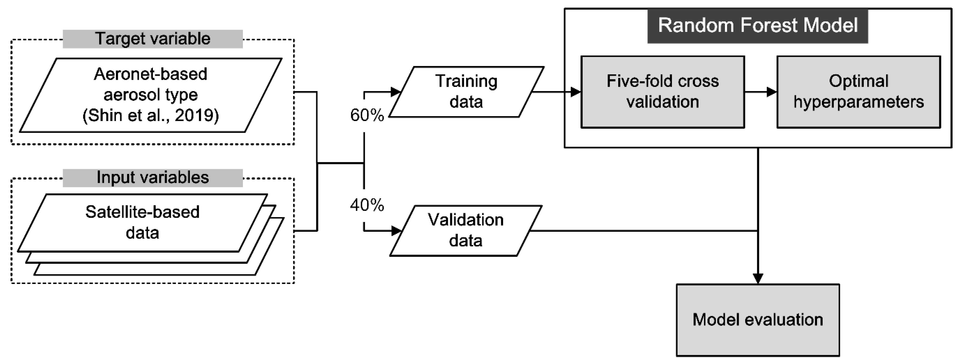
2.1. Description of Model

The RF is an ensemble of decision trees based on classification and regression trees in which multiple trees are aggregated with majority voting and averaged in classification regression tasks [26]. The RF method constructs numerous trees from bootstrap samples to overcome the common problem of over-fitting in decision-tree models. An ensemble model is based on bagging and randomized node optimization [26] and the RF method determines how input variables contribute to model development.
Figure 1 shows the overall process of the RF-based aerosol classification model. The RF model was trained using the AERONET aerosol type dataset (target variable) and various satellite input variables. The AERONET aerosol type dataset was constructed using the AERONET-based aerosol classification method proposed in [27]. This method identifies the seven aerosol types (pure dust; PD, dust dominant mixed; DDM, pollution dominant mixed; PDM, and pollution aerosols classified as strongly absorbing; SA, moderately absorbing; MA, weakly absorbing; WA, and non-absorbing; NA) using the SSA to determine aerosol absorbance and dust ratios (Rd) derived from a particle linear depolarization ratio at 1020 nm, which can distinguish contributions of non-spherical particles such as dust aerosols from the AERONET Version 3 product. Shin et al. [27] reported that Rd is a more suitable parameter for distinguishing aerosol types mixed with dust particles than FMF since non-spherical dust aerosols may occur in the fine mode. Threshold values used in classifying aerosol types from AERONET data are shown in Table 2. The AERONET version 3 Level 1.5 dataset was downloaded from the official website of the AERONET (https://aeronet.gsfc.nasa.gov/, accessed on 10 December 2020), operated by the National Aeronautics and Space Administration Goddard Space Flight Center.
The satellite input variable dataset was collected from TROPOMI data and aerosol optical properties from MODIS data. Satellite input variables of previous studies were utilized by Choi et al. [25], including AOD, AE, aerosol index, and trace-gas densities (CO and tropospheric NO2 column densities). Aerosol formation is reported to depend on radiation exposure, particularly its effect on smog production [28]. Since the amount of solar radiation depends on the solar zenith angle (SZA), Choi et al. [25] introduced the SZA as an input variable to indirectly represent aerosol formation by photochemical reactions. Top-of-atmosphere (TOA) reflectances at three wavelengths (412, 470, and 660 nm) were applied because they are dependent on the specific aerosol type, especially for aerosol absorbance [29]. Annual land-cover type and percentage urban area were selected to account for the effects of land-cover type on aerosol formation and to serve as proxies for aerosol source information [30,31]. The use of these 11 input variables allowed the RF-based model to account for the combined effects of trace-gas information with a classification accuracy of up to 73% [25]. However, the use of TROPOMI and MODIS measurements can result in loss of data owing to the collocation of satellite input variables. In this study, we attempted to exclude satellite input variables with many missing data and low MDA (i.e., variable importance).
Aerosol index, column densities of CO and tropospheric NO2, and SZA were obtained from TROPOMI level 2 products. The AOD, AE, and TOA reflectances were from a MODIS level 2 product (MYD04_L2). Annual land-cover type and percentage urban areas were obtained from a MODIS level 3 product (MCD12C1). MODIS products are available from NASA Level-1 and Atmosphere Archive and Distribution System of the Distributed Active Archive Center (https://ladsweb.modaps.eosdis.nasa.gov/, accessed on 22 September 2020).

2.2. Training and Validation of the RF Model

We trained the RF model using the ‘randomForest’ package (version 4.6-14) in Rstudio (R version 3.6.3). Hyperparameters of the RF model include ntree (binary classification trees), mtry (the number of input variables), and node size (the minimum size of terminal nodes). These hyperparameters must be optimized because model performance depends on them [26,32]. The ‘tune.randomForest’ function, used to obtain optimal hyperparameters such as ntree and node size, was obtained from the ‘e1071′ package (version 1.7-3). Node sizes of 1–5 with ntree values of 100–1500 were considered in tuning the hyperparameters. A single mtry value, the square root of the number of input variables, was applied as it is a value typically used for classification [33].
The dataset was randomly divided into separate training (60%) and test (40%) datasets. In the training procedure, k-fold (5-fold in this case) cross-validation was used to optimize hyperparameters with the training dataset randomly divided into five sets of the same size. Four folds were involved only in the training procedure, with the remaining single fold (unseen) being used to validate the performance of the trained model. This allowed us to choose optimized hyperparameters for best model performance, with 40% of the test dataset finally being used to evaluate the classification performance of the RF model.

3. Variable Importance and Data Volume for the Satellite Input Variable

We used data collected previously by Choi et al. [25] with the AERONET aerosol type dataset being obtained from AERONET Level 1.5 data (cloud-screened) as more data can be obtained from it than from AERONET Level 2.0 (quality-assured). Choi et al. [25] used only 440 nm AOD data above 0.4 to minimize uncertainties in AERONET Level 1.5 data; and collected AERONET aerosol type data at the overpass time (13:30 local time) of TROPOMI aboard the Sentinel-5P satellite and MODIS aboard the Aqua satellite for the period January 2018 to July 2020. The AERONET aerosol type dataset comprised 10,481 data points. After collection of the AERONET aerosol type dataset (N = 10,481), satellite variables (TROPOMI and MODIS data) were collocated by selecting the satellite pixel nearest the AERONET site to obtain training and validation datasets in AERONET site location, as in Choi et al. [25]. Three input variable sets were constructed for the selection of that with the highest classification accuracy, including all input variable candidates (11 variables), MODIS input variable candidates (7 variables), and TROPOMI input variable candidates (4 variables). The variable set with 11 input variables, including both TROPOMI and MODIS variables, was selected by Choi et al. [25] because of its higher classification accuracy (59%) than other variable sets. However, the input variable set with 11 parameters collected only 47% (N = 4906) of the total AERONET aerosol type dataset (N = 10,481) as many data were missing from each satellite product. The variable set including four TROPOMI variables (8693 data points) contains more data than the other sets with an overall accuracy of 51%. The set of MODIS variables (overall accuracy = 56%) contained only 5714 data points, with many data points missing except for annual land cover and percent of urban area.
In Choi et al. [25], variable importance for each satellite input parameter was investigated using the MDA value, which indicates the accuracy lost when a specific variable is excluded from the RF-based model (Table 3). The MDA of TROPOMI variables is 64–83% higher than that of MODIS variables apart from AOD. We excluded the input MODIS variables AE and TOA reflectance (at 412, 470, and 660 nm) due to their missing data and low importance. Despite its high MDA value, AOD was also excluded due to many missing data. We finally selected TROPOMI variables with low missing data and high MDA values; MODIS land cover type and percent of urban area variables were also selected as they comprise annual datasets with little missing data.

4. Results

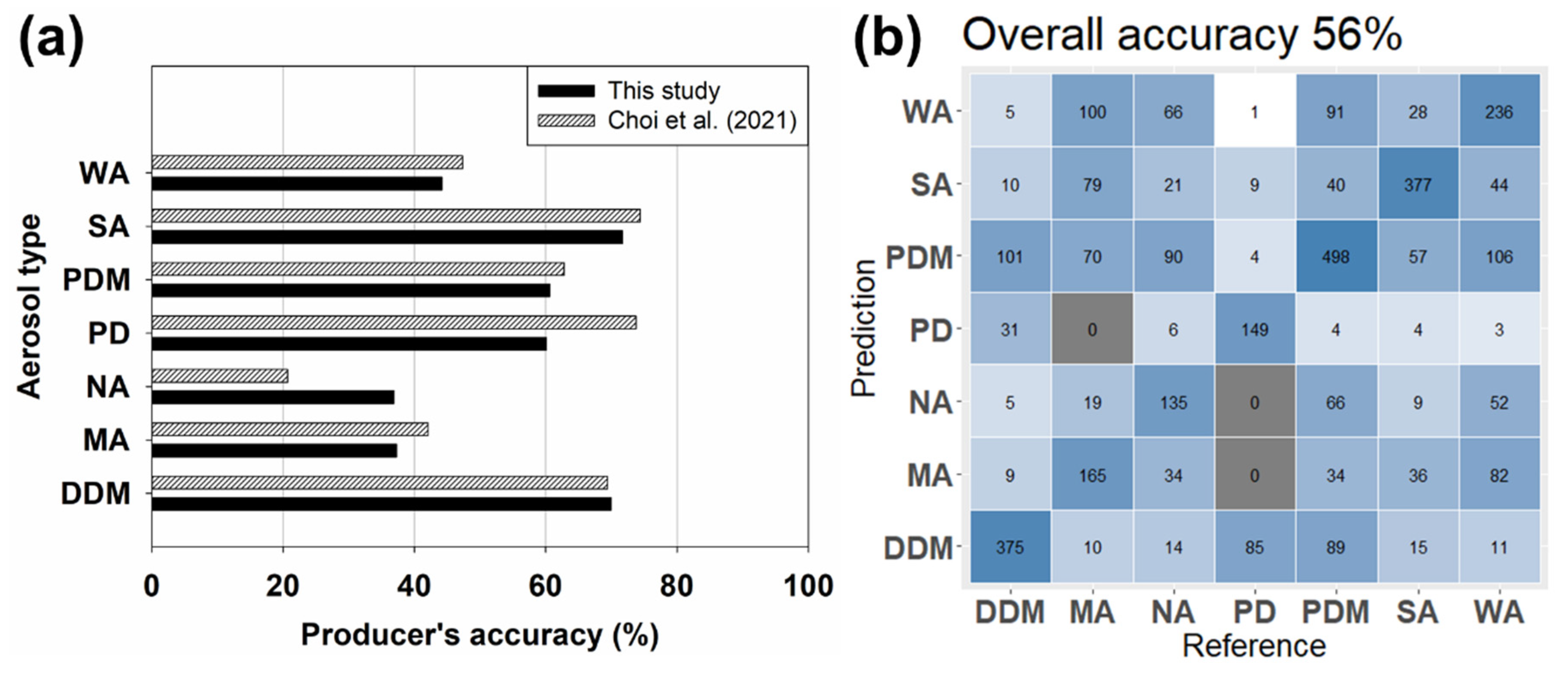
4.1. Assessment of the New RF-Based Model

A comparison was made between the RF-based model performance that was based on the variable set used by Choi et al. [25] and our selected set (Table 4). As found by Choi et al. [25], the data collection rate was only 47% when 11 TROPOMI and MODIS variables were used. When only two MODIS land-cover variables and four TROPOMI variables were used, the number of data points was maintained at N = 8693 and the overall accuracy in classifying the seven aerosol types was 56%, with a 5% increase over that when only TROPOMI variables were used. The difference in accuracy to the case where all 11 TROPOMI and MODIS variables were used was only 3%, with ~1.77 times more data being secured together with improved spatial coverage. The detailed comparison of spatial coverage between the RF-based model from Choi et al. [25] and this study is investigated in Section 4.2.
We investigated the confusion matrix and classification accuracy for each aerosol type to determine which are usually confused or well classified. Aerosol types that were usually confused with other types were merged based on a sensitivity test via confusion-matrix analysis
When aerosols were classified into the seven types (PD, DDM, PDM, SA, MA, WA, and NA), the overall accuracy (OA) of the RF-based model was 56%, with the classification performance for each type generally being comparable with but slightly poorer than those of Choi et al. [25], as shown in Figure 2a. Our RF-based model generally yielded reliable detection accuracies for the SA (72%), DDM (70%), PDM (61%), and PD (60%) types, indicating sensitivity to dust and pollution aerosols with strong absorption. The detection performance for pollution aerosols MA, WA, and NA was generally poor at <44%, similar to the performance observed by Choi et al. [25]. However, classification performance for the NA type (37%) was higher than the 21% achieved by Choi et al. [25], while the performance for the PD type was lower (60%, compared with 73%).
The RF-based model confuses mainly between the pollution-related aerosols (MA, WA, NA, and PDM) as shown in Figure 2b, and as reported by Choi et al. [25] who suggested that the difficulty for the RF-based model in discriminating between absorbing features of aerosols (except for the SA type) and identifying the PDM type that pollution and dust aerosols are mixed. Choi et al. [25] solved the problem of confusion between pollution-related aerosols by merging aerosols into the four classes PD, DDM, SA, and NA, achieving increased classification performance. We, therefore, merged the WA and NA types and the MA and SA types, while the PDM type was reclassified as the NA or SA type to integrate the PDM class into pollution aerosols.
The training process was repeated for the newly merged classes (SA, NA, DDM, and PD), with classification performance increasing from 56% to 73% (Figure 3b) i.e., the same OA as that achieved by Choi et al. [25] and with similar classification performance for TROPOMI and MODIS land-cover variables. In particular, our model yields a higher NA classification performance (77%) than that of Choi et al. (74%) [25] as shown in Figure 3a. Although PD classification performance was poorer than that achieved by Choi et al. [25], indicating decreased classification sensitivity for the PD type when using only TROPOMI variables and MODIS land-cover variables, our new classification model ensures extended spatial coverage with minimized input variables when classifying the four aerosol types.
Based on statistical validation, our RF-based model with TROPOMI and MODIS land-cover variables has acceptable accuracy. We attempted to evaluate the model using aerosol optical properties from AERONET data, as done by Choi et al. [25], who applied the spectral dependence of SSA to infer aerosol composition [25,34]. For example, SSA values of dust aerosols tend to increase with increasing wavelength, whereas those of carbonaceous aerosols decrease with increasing wavelength [34,35,36,37,38]. AERONET and RF-model aerosol types displayed similar trends in the wavelength dependence of SSA for each aerosol type (Figure 4a,b). In particular, the SSAs of PD and DDM tended to increase with wavelength, indicating a high contribution of dust aerosols. However, with the DDM type, the rate of SSA increase with wavelength is lower than that of PD, indicating that the RF-based model can distinguish PD and dust aerosols mixed with pollution aerosols. With the SA type, SSA values tend to decrease with increasing wavelength, indicating that the AERONET and RF algorithms reasonably describe the wavelength dependence of carbonaceous aerosol types, consistent with previous studies [27,34,35,36].
The performance of the RF-based model was assessed quantitatively by comparing SSA values at wavelengths of 440, 675, 870, and 1020 nm for AERONET aerosol types (Figure 4a) with those of the RF-based model (Figure 4b), with differences between the two shown in Figure 4c,d. The mean differences in SSA at 440, 675, 870, and 1020 nm were 0.003, 0.005, 0.007, and 0.008, respectively, similar to those values reported by Choi et al. [25] (averaging <0.01). Although the difference in SSA is <0.01, the internal uncertainty of AERONET SSA (0.03) [39] must be considered.
The effect of merging aerosol types on classification performance, in terms of aerosol optical properties (SSA values at 440, 675, 870, and 1020 nm, FMF, and Rd values) is shown in Table 5, which summarizes means and standard deviations of differences between AERONET and RF aerosol types. All of these parameters tended to decrease when aerosol types were merged. For example, with seven aerosol types, the differences in SSA at 440, 675, 870, and 1020 nm were 0.006, 0.010, 0.013, and 0.015, respectively, and with four aerosol classes, the differences were 0.003, 0.005, 0.007, and 0.008, respectively. The difference in Rd values also decreased from 0.061 to 0.027 through the merging of aerosol classes, while differences in FMF values were relatively unaffected. The decreasing trends in aerosol optical properties indicate that merging aerosol classes contributed to a decrease in classification confusion in the satellite aerosol classification model.

4.2. Spatial Distributions among DIfferent Aerosol Classification Models

Figure 5 shows aerosol types classified by the RF-based algorithm with fewer variables (this study), that of Choi et al. [25], and the threshold-based algorithms [9,12] on 26 March, 2018. The aerosols were classified for pixels where the TROPOMI cloud fraction is <0.2 and SZA is <70° to reduce uncertainties in input variables due to the presence of cloud and a high solar zenith angle. Over the ocean, we classified aerosols with high aerosol loadings (AOD > 0.4) for our RF-based algorithm and that from Torres et al. [9], because these algorithms do not classify sea salt aerosols. In the case of the aerosol classification from Lee et al. [12], aerosols were classified over the ocean for all aerosol loading because Lee et al. [12] classify sea salt aerosols.
As shown in Figure 5a–d, on 26 March, 2018, aerosols were classified over 2,149,917 and 823,505 pixels using the RF-based model used here and that of Choi et al. [25], respectively. The reduction in input variables was found to greatly improve spatial coverage of the RF-based model. In general, spatial distributions of aerosol types classified by RF-based algorithms tend to be similar, except over parts of South America (including the Atacama, Monte, and Patagonian Deserts), South Africa (including Namib and Kalahari deserts), and Australia (including Strzelecki and Simpson Deserts). Over these regions, the RF-based model used here (Figure 5a,b) classified aerosol types as PD or DDM (dust; i.e., coarse-mode absorbing aerosols), whereas that of Choi et al. [25] (Figure 5c,d) classified them as SA (fine-mode absorbing aerosols). To clarify the difference in aerosol classification, we investigated AE values from the AERONET site. Near the overpass time (13:30) of the TROPOMI (aboard Sentinel-5p) and MODIS (aboard Aqua), the AERONET data were only measured observed over CEILAP-Neuquen (South America) and Gobabeb (South Africa) with AE values of 0.48 and 0.59, respectively, indicating the likely presence of coarse-mode aerosols. It may be possible to determine whether the coarse-mode aerosol is present when lidar observation data with polarization capabilities are available in the future. Therefore, the dust aerosols (PD or DDM) are more appropriate than the pollution aerosols (SA) over the regions. For the part of Australia, more investigations are needed for case studies in the future. The PD type was detected with high aerosol loadings (average AOD: 0.98) over the North Atlantic Ocean between the Sahara Desert and North America. The average (maximum) MODIS AE and TROPOMI AI were found to be 0.29 (0.59) and 0.51 (2.15), respectively, indicating the presence of dust aerosols may be transported from the Sahara Desert. In order to check the transport of dust aerosols from the Sahara Desert, a hybrid single-particle Lagrangian integrated trajectory (HYSPLIT) model was used [40,41]. Figure 6 shows 96-h HYSPLIT back trajectories (1-degree Global Data Assimilation System, GDAS meteorology) originating from 500, 1000, and 1500 m above ground level (AGL) at the point of dust plume detected over the North Pacific Ocean (latitude: 10, longitude: −30). Based on backward trajectory analysis, it was found that a dust plume detected over the North Pacific Ocean is transported from the Sahara Desert.
Aerosol types classified by earlier threshold-based algorithms [9,12] have high spatial coverages (2,342,921 pixels for Torres et al. [9]; 1,486,496 pixels for Lee et al. [12]), as shown in Figure 5e,f. Torres et al. [9] are found to have the highest spatial coverage especially over the land (Figure 5e). Furthermore, Lee et al. [12] classify aerosols for the much more data points over the ocean with sea salt aerosols. However, these earlier classification models [9,12] give a much higher difference in SSA values (0.0265–0.0513 for Torres et al. [9]; 0.0190–0.0337 for Lee et al. [12]) than those of the RF-based model (<0.01) [25]. The RF-based algorithm used here yields improved spatial coverage with performance comparable with that used by Choi et al. [25].

5. Discussion

Previous studies generally used a threshold-based approach for identifying aerosol types with satellite input variables [9,13,14,15,16], with aerosol optical properties and trace-gas information (with internal uncertainties) being obtained from various satellite sensors. Although uncertainties in satellite input parameters may lead to misclassification of aerosols, the early methods were rarely evaluated as reported in [25]. The RF classification model of Choi et al. [25] was evaluated using AERONET aerosol optical properties with reasonable classification performance being achieved, but with limitations on spatial coverage due to missing data of each satellite product.
Both Choi et al. [25] and this study applied a random forest model to classify satellite aerosol types, with this study attempting to improve spatial coverage of the RF model by reducing the number of input variables. In this study, we followed the work of Choi et al. [25] to improve spatial coverage of the RF aerosol classification model. Among the 11 input variables used by Choi et al. [25], we excluded satellite input variables with many missing data points or low variable importance. The reduced satellite input variables include four TROPOMI-based variables (aerosol index, tropospheric CO and NO2 column densities, and SZA) and two MODIS-based variables (annual land-cover type and percentage urban ratio). The performance of the RF-based model with a reduced number of variables is similar to that of the model with 11 variables used by Choi et al. [25], although with a reduction in input variables the model may not fully distinguish pure dust aerosols, especially with MODIS aerosol optical variables being excluded. However, the reduction in input variables led to improved spatial coverage over the satellite aerosol classification model.
Our satellite aerosol classification model was evaluated with the AERONET-based aerosol type dataset constructed by Shin et al. [27] and aerosol optical properties of typical aerosol types. In future work, our results should be compared with other ground-based aerosol classification methods. Hamil et al. [42], Ozdemir et al. [43], and Stefan et al. [44] suggested aerosol classification methods using mainly parameters related to aerosol size and scattering properties based on AERONET measurement data, with Kaskaoutis [45] combining in situ measurement data to classify aerosol types for the first time.

6. Summary and Conclusions

We improved the spatial coverage of the RF aerosol type classification model. Satellite input variables with many missing data points and of low importance were excluded from the final input variable set. Four TROPOMI input variables (aerosol index, tropospheric CO and NO2 column densities, and SZA) and two MODIS variables (annual land-cover type and percentage urban area) were selected. The RF-based model with these reduced input variables gave a performance comparable to that of the model with 11 input variables. The global spatial coverage of the RF algorithm was compared with that of previous methods, with the RF-based model providing improved spatial coverage while maintaining a classification performance comparable with that of other models.
It is necessary for future studies to improve the accuracy of the aerosol type classification algorithm of the RF-based model through the use of additional variables (with fewer missing data), such as meteorological data from numerical weather prediction models and chemical variables from chemical-transport models. Furthermore, the collection of a longer-term dataset should improve the accuracy of the model, which may provide aerosol type information with spatially continuous coverage, providing global climatological distributions of aerosol types even where there are no AERONET sites.

Author Contributions

Conceptualization, H.L.; methodology, W.C.; validation, W.C.; writing—original draft preparation, W.C.; writing—review and editing, H.L.; investigation, D.K., S.K. All authors have read and agreed to the published version of the manuscript.

Funding

This work was supported by the National Research Foundation of Korea (NRF) grant funded by the Korea government (MSIP) (No. 2019R1F1A1058295).

Institutional Review Board Statement

Not applicable.

Informed Consent Statement

Not applicable.

Data Availability Statement

For the results and data generated during the study, please contact the first author.

Acknowledgments

The authors would like to thank the U.S. NASA providing MODIS Collection 6.1 aerosol product and AERONET data. We also thank ESA for making possible the distribution of TROPOMI data. This work was performed within the framework of the Sentinel 5P Calibration & Validation (S5P Cal/Val) Project.

Conflicts of Interest

The authors declare no conflict of interest.

References

  1. Bréon, F.M.; Goloub, P. Cloud droplet effective radius from spaceborne polarization measurements. Geophys. Res. Lett. 1998, 25, 1879–1882. [Google Scholar] [CrossRef]
  2. Chen, Q.; Yuan, Y.; Huang, X.; He, Z.; Tan, H. Assessment of column aerosol optical properties using ground-based sun-photometer at urban Harbin, Northeast China. J. Environ. Sci. 2018, 74, 50–57. [Google Scholar] [CrossRef]
  3. Stocker, T. Climate Change 2013: The Physical Science Basis: Working Group I Contribution to the Fifth Assessment Report of the Intergovernmental Panel on Climate Change; Cambridge University Press: Cambridge, UK, 2014. [Google Scholar]
  4. Mao, Q.; Huang, C.; Zhang, H.; Chen, Q.; Yuan, Y. Aerosol optical properties and radiative effect under different weather conditions in Harbin, China. Infrared Phys. Technol. 2018, 89, 304–314. [Google Scholar] [CrossRef]
  5. Charlson, R.J.; Schwartz, S.; Hales, J.; Cess, R.D.; Coakley, J.J.; Hansen, J.; Hofmann, D. Climate forcing by anthropogenic aerosols. Science 1992, 255, 423–430. [Google Scholar] [CrossRef]
  6. Christopher, S.A.; Zhang, J. Daytime variation of shortwave direct radiative forcing of biomass burning aerosols from GOES-8 imager. J. Atmos. Sci. 2002, 59, 681–691. [Google Scholar] [CrossRef] [Green Version]
  7. Procopio, A.S.; Artaxo, P.; Kaufman, Y.J.; Remer, L.A.; Schafer, J.S.; Holben, B.N. Multiyear analysis of amazonian biomass burning smoke radiative forcing of climate. Geophys. Res. Lett. 2004, 31, L03108. [Google Scholar] [CrossRef]
  8. Takemura, T.; Nakajima, T.; Dubovik, O.; Holben, B.N.; Kinne, S. Single-scattering albedo and radiative forcing of various aerosol species with a global three-dimensional model. J. Clim. 2002, 15, 333–352. [Google Scholar] [CrossRef]
  9. Higurashi, A.; Nakajima, T. Detection of aerosol types over the East China Sea near Japan from four-channel satellite data. Geophys. Res. Lett. 2002, 29, 17-11–17-14. [Google Scholar] [CrossRef]
  10. Kaskaoutis, D.; Kambezidis, H. Comparison of the Ångström parameters retrieval in different spectral ranges with the use of different techniques. Meteorol. Atmos. Phys. 2008, 99, 233–246. [Google Scholar] [CrossRef]
  11. Remer, L.A.; Kaufman, Y.; Tanré, D.; Mattoo, S.; Chu, D.; Martins, J.V.; Li, R.-R.; Ichoku, C.; Levy, R.; Kleidman, R. The MODIS aerosol algorithm, products, and validation. J. Atmos. Sci. 2005, 62, 947–973. [Google Scholar] [CrossRef] [Green Version]
  12. Torres, O.; Ahn, C.; Chen, Z. Improvements to the OMI near-UV aerosol algorithm using A-train CALIOP and AIRS observations. Atmos. Meas. Technol. 2013, 6, 3257–3270. [Google Scholar] [CrossRef] [Green Version]
  13. Jeong, M.J.; Li, Z. Quality, compatibility, and synergy analyses of global aerosol products derived from the advanced very high resolution radiometer and Total Ozone Mapping Spectrometer. J. Geophys. Res. Atmos. 2005, 110, D10S08. [Google Scholar] [CrossRef] [Green Version]
  14. Kim, J.; Lee, J.; Lee, H.C.; Higurashi, A.; Takemura, T.; Song, C.H. Consistency of the aerosol type classification from satellite remote sensing during the Atmospheric Brown Cloud–East Asia Regional Experiment campaign. J. Geophys. Res. Atmos. 2007, 112, D22S33. [Google Scholar] [CrossRef]
  15. Lee, J.; Kim, J.; Lee, H.C.; Takemura, T. Classification of aerosol type from MODIS and OMI over East Asia. Asia-Pac. J. Atmos. Sci. 2007, 43, 343–357. [Google Scholar]
  16. Mao, Q.; Huang, C.; Chen, Q.; Zhang, H.; Yuan, Y. Satellite-based identification of aerosol particle species using a 2D-space aerosol classification model. Atmos. Environ. 2019, 219, 117057. [Google Scholar] [CrossRef]
  17. Penning de Vries, M.; Beirle, S.; Hörmann, C.; Kaiser, J.; Stammes, P.; Tilstra, L.; Wagner, T. A global aerosol classification algorithm incorporating multiple satellite data sets of aerosol and trace gas abundances. Atmos. Chem. Phys. 2015, 15, 10597–10618. [Google Scholar] [CrossRef] [Green Version]
  18. Omar, A.H.; Winker, D.M.; Vaughan, M.A.; Hu, Y.; Trepte, C.R.; Ferrare, R.A.; Lee, K.P.; Hostetler, C.A.; Kittaka, C.; Rogers, R.R.; et al. The CALIPSO automated aerosol classification and lidar ratio selection algorithm. J. Atmos. Ocean. Technol. 2009, 26, 1994–2014. [Google Scholar] [CrossRef]
  19. Vaughan, M.A.; Young, S.A.; Winker, D.M.; Powell, K.A.; Omar, A.H.; Liu, Z.; Hu, Y.; Hostetler, C.A. Fully automated analysis of space-based lidar data: An overview of the CALIPSO retrieval algorithms and data products. In Laser radar techniques for atmospheric sensing. Int. Soc. Opt. Photonics 2004, 5575, 16–30. [Google Scholar]
  20. Chu, D.; Kaufman, Y.; Ichoku, C.; Remer, L.; Tanré, D.; Holben, B. Validation of MODIS aerosol optical depth retrieval over land. Geophys. Res. Lett. 2002, 29, MOD2-1–MOD2-4. [Google Scholar] [CrossRef] [Green Version]
  21. Qi, Y.; Ge, J.; Huang, J. Spatial and temporal distribution of MODIS and MISR aerosol optical depth over northern China and comparison with AERONET. Chin. Sci. Bull. 2013, 58, 2497–2506. [Google Scholar] [CrossRef] [Green Version]
  22. Thrastarson, H.T.; Manning, E.; Kahn, B.; Fetzer, E.; Yue, Q.; Wong, S.; Kalmus, P.; Payne, V.; Olsen, E. AIRS/AMSU/HSB Version 7 Level 2 Product User Guide; Jet Propulsion Laboratory, California Institute of Technology: Pasadena, CA, USA, 2020; pp. 83–92. [Google Scholar]
  23. Papagiannopoulos, N.; Mona, L.; Alados-Arboledas, L.; Amiridis, V.; Baars, H.; Binietoglou, I.; Bortoli, D.; D’Amico, G.; Giunta, A.; Guerrero-Rascado, J.L.; et al. CALIPSO climatological products: Evaluation and suggestions from EARLINET. Atmos. Chem. Phys. 2016, 16, 2341–2357. [Google Scholar] [CrossRef] [Green Version]
  24. Holben, B.N.; Eck, T.F.; Slutsker, I.A.; Tanre, D.; Buis, J.P.; Setzer, A.; Vermote, E.; Reagan, J.A.; Kaufman, Y.J.; Nakajima, T.; et al. AERONET—A federated instrument network and data archive for aerosol characterization. Remote Sens. Environ. 1998, 66, 1–16. [Google Scholar] [CrossRef]
  25. Choi, W.; Lee, H.; Park, J. A First Approach to Aerosol Classification using Space-Borne Measurement Data: Machine Learning-based Algorithm and Evaluation. Remote Sens. 2021, 13, 609. [Google Scholar] [CrossRef]
  26. Breiman, L. Random forests. Mach. Learn. 2001, 45, 5–32. [Google Scholar] [CrossRef] [Green Version]
  27. Shin, S.-K.; Tesche, M.; Noh, Y.; Müller, D. Aerosol-type classification based on AERONET version 3 inversion products. Atmos. Meas. Technol. 2019, 12, 3789–3803. [Google Scholar] [CrossRef] [Green Version]
  28. Dickerson, R.; Kondragunta, S.; Stenchikov, G.; Civerolo, K.; Doddridge, B.; Holben, B. The impact of aerosols on solar ultraviolet radiation and photochemical smog. Science 1997, 278, 827–830. [Google Scholar] [CrossRef] [Green Version]
  29. Tao, M.; Chen, L.; Wang, Z.; Wang, J.; Che, H.; Xu, X.; Wang, W.; Tao, J.; Zhu, H.; Hou, C. Evaluation of MODIS Deep Blue aerosol algorithm in desert region of East Asia: Ground validation and intercomparison. J. Geophys. Res. Atmos. 2017, 122, 10357–10368. [Google Scholar] [CrossRef]
  30. Wu, S.; Mickley, L.J.; Kaplan, J.; Jacob, D.J. Impacts of changes in land use and land cover on atmospheric chemistry and air quality over the 21st century. Atmos. Chem. Phys. 2012, 12, 1597–1609. [Google Scholar] [CrossRef] [Green Version]
  31. Fu, Y.; Liao, H. Impacts of land use and land cover changes on biogenic emissions of volatile organic compounds in China from the late 1980s to the mid-2000s: Implications for tropospheric ozone and secondary organic aerosol. Tellus B 2014, 66, 24987. [Google Scholar] [CrossRef]
  32. Mutanga, O.; Adam, E.; Cho, M.A. High density biomass estimation for wetland vegetation using WorldView-2 imagery and random forest regression algorithm. Int. J. Appl. Earth Obs. Geoinf. 2012, 18, 399–406. [Google Scholar] [CrossRef]
  33. Probst, P.; Wright, M.N.; Boulesteix, A.L. Hyperparameters and tuning strategies for random forest. Wiley Data Min. Knowl. Discov. 2019, 9, e1301. [Google Scholar] [CrossRef] [Green Version]
  34. Li, J.; Carlson, B.E.; Lacis, A.A. Using single-scattering albedo spectral curvature to characterize East Asian aerosol mixtures. J. Geophys. Res. Atmos. 2015, 120, 2037–2052. [Google Scholar] [CrossRef]
  35. Dubovik, O.; Holben, B.; Eck, T.F.; Smirnov, A.; Kaufman, Y.J.; King, M.D.; Tanré, D.; Slutsker, I. Variability of absorption and optical properties of key aerosol types observed in worldwide locations. J. Atmos. Sci. 2002, 59, 590–608. [Google Scholar] [CrossRef]
  36. Meloni, D.; Di Sarra, A.; Pace, G.; Monteleone, F. Aerosol optical properties at Lampedusa (Central Mediterranean). 2. Determination of single scattering albedo at two wavelengths for different aerosol types. Atmos. Chem. Phys. 2006, 6, 715–727. [Google Scholar] [CrossRef] [Green Version]
  37. Eck, T.F.; Holben, B.N.; Sinyuk, A.; Pinker, R.; Goloub, P.; Chen, H.; Chatenet, B.; Li, Z.; Singh, R.; Tripathi, S.; et al. Climatological aspects of the optical properties of fine/coarse mode aerosol mixtures. J. Geophys. Res. 2010, 115, D19205. [Google Scholar] [CrossRef] [Green Version]
  38. Derimian, Y.; Karnieli, A.; Kaufman, Y.J.; Andreae, M.O.; Andreae, T.W.; Dubovik, O.; Maenhaut, W.; Koren, I. The role of iron and black carbon in aerosol light absorption. Atmos. Chem. Phys. 2008, 8, 3623–3637. [Google Scholar] [CrossRef] [Green Version]
  39. Sinyuk, A.; Holben, B.N.; Eck, T.F.; Giles, D.M.; Slutsker, I.; Korkin, S.; Schafer, J.S.; Smirnov, A.; Sorokin, M.; Lyapustin, A. The AERONET Version 3 aerosol retrieval algorithm, associated uncertainties and comparisons to Version 2. Atmos. Meas. Tech. 2020, 13, 3375–3411. [Google Scholar] [CrossRef]
  40. Stein, A.F.; Draxler, R.R.; Rolph, G.D.; Stunder, B.J.B.; Cohen, M.D.; Ngan, F. NOAA’s HYSPLIT atmospheric transport and dispersion modeling system. Bull. Amer. Meteor. Soc. 2015, 96, 2059–2077. [Google Scholar] [CrossRef]
  41. Rolph, G.; Stein, A.; Stunder, B. Real-time Environmental Applications and Display sYstem: READY. Environ. Model. Softw. 2017, 95, 210–228. [Google Scholar] [CrossRef]
  42. Hamill, P.; Giordano, M.; Ward, C.; Giles, D.; Holben, B. An AERONET-based aerosol classification using the Mahalanobis distance. Atmos. Environ. 2016, 140, 213–233. [Google Scholar] [CrossRef]
  43. Ozdemir, E.; Tuygun, G.T.; Elbir, T. Application of aerosol classification methods based on AERONET version 3 product over eastern Mediterranean and Black Sea. Atmos. Poll. Res. 2020, 11, 2226–2243. [Google Scholar] [CrossRef]
  44. Stefan, S.; Voinea, S.; Iorga, G. Study of the aerosol optical characteristics over the Romanian Black Sea Coast using AERONET data. Atmos. Poll. Res. 2020, 11, 1165–1178. [Google Scholar] [CrossRef]
  45. Kaskaoutis, D.G.; Grivas, G.; Stavroulas, I.; Liakakou, E.; Dumka, U.C.; Dimitriou, K.; Gerasopoulos, E.; Mihalopoulos, N. In situ identification of aerosol types in Athens, Greece, based on long-term optical and on online chemical characterization. Atmos. Environ. 2021, 246, 118070. [Google Scholar] [CrossRef]
Figure 1. Schematic diagram of random forest (RF) aerosol classification model.
Remotesensing 13 01268 g001
Figure 2. (a) producer’s accuracy (PA) and (b) confusion matrix for each aerosol with the classification of seven aerosol types (PD, DDM, PDM, SA, MA, WA, and NA).
Remotesensing 13 01268 g002
Figure 3. (a) PA and (b) confusion matrix for each aerosol in the classification of the four aerosol types (PD, DDM, SA, and NA).
Remotesensing 13 01268 g003
Figure 4. Wavelength dependence of single-scattering albedo (SSA) at 440, 675, 870, and 1020 nm for (a) AERONET aerosol types and (b) RF aerosol types (this study); (c) the absolute difference in SSA for each aerosol type; (d) average differences in SSA. Error bars represent the standard deviation of the SSA difference. The gray-colored graphs indicate the values suggested by Choi et al. [25].
Remotesensing 13 01268 g004
Figure 5. Comparisons of spatial distributions of aerosol types classified from (a) RF-based algorithm with a reduced number of input variables in this study (four type classification), (b) RF-based algorithm with a reduced number of input variables in this study (seven type classification), (c) RF-based algorithm in Choi et al. [25] (four type classification), (d) RF-based algorithm in Choi et al. [25] (seven type classification), (e) Torres et al. [9], and (f) Lee et al. [12] on 26 March 2018.
Remotesensing 13 01268 g005
Figure 6. 96-h backward trajectories at 500, 1000, 1500 m AGL on 26 March 2018.
Remotesensing 13 01268 g006
Table 1. Summary of previous studies of threshold-based satellite aerosol classification. Abbreviations: SeaWiFS, Sea-viewing Wide Field-of-view Sensor; AVHRR, Advanced Very-High-Resolution Radiometer; TOMS, total-ozone mapping spectrometer; MODIS, Moderate-Resolution Imaging Spectroradiometer; OMI, Ozone Monitoring Instrument; GOME-2, Second Global Ozone Monitoring Experiment; MOPITT, Measurements of Pollution in the Troposphere.
ReferenceParametersAerosol Types Validation
(or Comparison)
Higurashi and Nakajima [9]Spectral radiances in channels 1, 2, 6, and 8 of SeaWiFS (center wavelength: 412, 443, 670, and 865 nm)Soil dust, carbonaceous, sulfate, and sea salt-
Jeong and Li [13]Aerosol optical thickness and Ångström exponent from AVHRR
Aerosol optical thickness and Aerosol index from TOMS
Biomass burning, dust, sea salt, and four mixtures -
Kim et al. [14]Fine mode fraction from MODIS
Aerosol index from OMI
Carbonaceous, dust, sulfate, sea salt, and five mixturesAgreement with aerosol classification from Higurashi and Nakajima [9]: 32–81%
Lee et al. [15]Aerosol optical thickness and Ångström exponent from MODIS
Aerosol index from OMI
Dust, sea salt, smoke,
and sulfate and two mixtures
Comparison with global aerosol climate model
Torres et al. [12] Column amount of CO from AIRS
Aerosol index from OMI
Desert dust, carbonaceous particles, and sulfate-based aerosols-
Penning de Vries et al. [17]Aerosol optical depth from MODIS
Aerosol index, column amounts of NO2, HCHO, SO2 from GOME-2
Column amount of CO from MOPITT
Biomass burning smoke, desert dust, secondary aerosols of biogenic origin, secondary aerosols of urban/industrial origin, aged aerosols, volcanic sulfate, sea salt, unknown source Comparison with model-derived aerosol compositions from the global
monitoring atmospheric composition and climate model.
Mao et al. [16]Aerosol relative optical depth from MODISDesert dust, continental, sub-continental, urban industry, biomass burningAgreement with ground-based aerosol type data: 36–91%
Table 2. Threshold values used in classifying aerosol types using AERONET measurement data.
Aerosol TypeThreshold
Pure dust (PD)0.89 < Rd
dust dominated mixed (DDM)0.53 ≤ Rd ≤ 0.89
pollution dominated mixed (PDM)0.17 ≤ Rd < 0.53
non-absorbing (NA)Rd < 0.170.95 < SSA
weakly absorbing (WA)0.90 < SSA ≤ 0.95
moderately absorbing (MA)0.85 ≤ SSA ≤ 0.90
strongly absorbing (SA)SSA < 0.85
Table 3. List of satellite input variables and variable importance [25].
Sensor (Mission)Product (Level)Variable NameVariable Importance (MDA)
TROPOMI (Sentinel-5P)AI (L2)Aerosol Index83%
Solar Zenith Angle76%
CO (L2)CO column amount70%
NO2 (L2)Tropospheric NO2 column density64%
MODIS (Aqua)MYD04 (L2)Aerosol Optical Depth at 550 nm82%
Ångström Exponent
(wavelength pair: 550 nm and 860 nm)
54%
Deep blue TOA reflectance at 412 nm52%
Deep blue TOA reflectance at 470 nm49%
Deep blue TOA reflectance at 660 nm61%
MCD12C1 (L3)Land cover type61%
Percent of urban area57%
Table 4. Summary of variables, data, and overall accuracy for the initial input variable set.
Dataset NameInput VariablesThe Number of DataOverall Accuracy (%)
TotalTraining (60%)Test (40%)
Choi et al. [25]
(11 variables)
TROPOMI- Aerosol index
- Solar zenith angle
- CO column amount
- Tropospheric NO2 column density
49062946196059%
MODIS- Aerosol optical depth (at 550 nm)
- Ångström exponent (wavelength pair: 550 nm and 860 nm)
- Deep blue TOA reflectance at 412, 470, and 660 nm
- Land cover type (annual)
- Percent of urban area (annual)
This study
(6 variables)
TROPOMI- Aerosol index
- Solar zenith angle
- CO column amount
- Tropospheric NO2 column density
86935218347556%
MODIS- Land cover type (annual)
- Percent of urban area (annual)
Table 5. Means and standard deviations of differences in SSAs, fine-mode fraction (FMF), and aerosol absorbance and dust ratios (Rd) values for several aerosol classification models identifying seven or four aerosol types. Values in parentheses are from Choi et al. [25].
Seven Aerosol Classes
(PD, DDM, PDM, SA, MA, WA, and NA)
Four Aerosol Classes
(PD, DDM, SA, and NA)
AverageStandard DeviationAverageStandard Deviation
SSA4400.006 (0.007)0.007 (0.006)0.003 (0.002)0.004 (0.003)
SSA6750.010 (0.008)0.009 (0.009)0.005 (0.004)0.006 (0.005)
SSA8700.013 (0.010)0.011 (0.011)0.007 (0.005)0.008 (0.007)
SSA10200.015 (0.012)0.013 (0.012)0.008 (0.006)0.009 (0.008)
FMF0.012 (0.027)0.014 (0.020)0.011 (0.005)0.018 (0.006)
Rd0.061 (0.047)0.017 (0.016)0.027 (0.016)0.037 (0.019)
Overall accuracy56% (59%)73% (73%)
Publisher’s Note: MDPI stays neutral with regard to jurisdictional claims in published maps and institutional affiliations.

