Ocean-Surface Heterogeneity Mapping (OHMA) to Identify Regions of Change

Abstract

Mapping heterogeneity of the ocean’s surface waters is important for understanding biogeographical distributions, ocean surface habitat mapping, and ocean surface stability. This article describes the Ocean-surface Heterogeneity MApping (OHMA) algorithm—an objective, replicable approach that uses hypertemporal, satellite-derived datasets to map the spatio-temporal heterogeneity of ocean surface waters. The OHMA produces a suite of complementary datasets—a surface spatio-temporal heterogeneity dataset, and an optimised spatio-temporal classification of the ocean surface. It was demonstrated here using a hypertemporal Sea Surface Temperature image dataset of the North Atlantic. Validation with Underway-derived temperature data showed higher heterogeneity areas were associated with stronger surface temperature gradients, or an increased presence of locally extreme temperature values. Using four exploratory case studies, spatio-temporal heterogeneity values were related to a range of region-specific surface and sub-surface characteristics including fronts, currents and bathymetry. The values conveyed the interactions between these parameters as a single metric. Such over-arching heterogeneity information is virtually impossible to map from in-situ instruments, or less temporally dense satellite datasets. This study demonstrated the OHMA approach is a useful and robust tool to explore, examine, and describe the ocean’s surface. It advances our capability to map biologically relevant measures of ocean surface heterogeneity. It can support ongoing efforts in Ocean Surface Partitioning, and attempts to understand marine species distributions. The study highlighted the need to establish dedicated spatio-temporal ocean validation sites, specifically measured using surface transits, to support advances in hypertemporal ocean data use, and exploitation. A number of future research avenues are also highlighted.

1. Introduction

1.1. Heterogeneity, and the Ocean-Surface

The world is heterogeneous and non-equilibrial [1]. This heterogeneity is underpinned by complexity and/or variability, as properties change over space and/or time [2]. The ocean structure, for example, is shaped by changes in water properties (e.g., temperature, salinity, nutrient content) and water movement in space and time. When water masses interact, they create a 4-dimensional architecture which is more structurally complex, and spatio-temporally variable. These confluence zones, or discontinuities, offer a wide variety of different habitats and niches, supporting rich biodiversity [3]. Longhurst notes that biogeographical or ecological regional boundaries will be clearest where discontinuities in the physical environment are strongest, such as along major fronts in the open ocean [4]. These boundary areas often feature the mixing of cold nutrient-rich water, with warmer nutrient-poor water, are more physically complex regions, and are often recognised as areas of high productivity ([4,5,6]). Complexity strongly affects the structure and dynamics of ecological communities. Increased complexity is often linked to greater species diversity and abundance [7,8], and is known to enhance ecosystem stability [9] and resilience [10]. It is also important to acknowledge the role of more homogenous patches, in a region’s heterogeneity. Here, transitions are less abrupt, and water properties are simply different to those further away, providing an element of patchiness to a region’s heterogeneity.

Mapping of terrestrial landscape spatio-temporal heterogeneity has been used to identify highly variable regions, highlighting the effects of stronger and dominant environmental gradients [11]. For clarity, in this study Surface spatio-Temporal Heterogeneity (STH) refers to the variability in an ocean-surface property across space and time. Mapping it can aid the understanding of interactions between ocean-surface systems. For example, Gratwicke gives a good summary of efforts to quantify the effects of hard, sub-surface complexity on marine life at local scales, and notes a need for habitat complexity to be considered when investigating fish biodiversity [12]. However, in the open ocean, the structural nature of the surface is largely determined by mobile boundaries between water masses of differing salinity, temperature, and nutrient content. Margalef noted that fronts in the ocean can be considered both as boundaries and as habitats in themselves, having the attributes of ecotones [13] or transition zones between ecological communities which are linear, and less extensive than the communities they separate [14]. There have been numerous studies which have identified areas of front persistence, or high front frequency (for example see [5,15]), as regions of enhanced regional biodiversity, and species abundance. Their surface expressions, which are the only features detectable using satellite sensors, represent far more extensive structures beneath the surface, shaping the distribution of life beneath the surface [16,17,18], and driving the region’s ecosystem functioning [6]. STH features vary regionally. Where the transition is not sharp enough to be delineated as a front, a gradual transition zone still separates different water masses. These soft and hard boundaries also move over space, and time, particularly in the ocean. Indeed, some regions could be characterised by their inconsistency, in terms of the presence and absence of frontal systems and water masses. It is important to recognise this, especially when examining how a region’s characteristic instability may drive the distribution of life. For example, the presence of strong upwellings can fuel enhanced productivity in some regions (e.g., the Canaries Upwelling Ecosystem [19]). Elsewhere it can be the effect of strong Western boundary currents and their associated structures (e.g., [20] and [21]) which drive regional heterogeneity, and fuel productivity.

From the species perspective, area dependencies can take years, or even decades, to develop. Therefore, it would be useful to develop a comprehensive measure of heterogeneity that aligns with biological activity, and timeframes. This measure should allow (i) an objective view of an ocean region’s spatio-temporal heterogeneity, (ii) the possibility to compare heterogeneity inter-annually and inter-seasonally, and (iii) measurements at biologically relevant timeframes and spatial scales, (to support studies into niche suitability and exploitation). By adopting approaches which are focused on STH itself, this wider range of regional variability could be examined more comprehensively. This could allow the diversity of habitats to be better quantified, and improve mapping of ocean-surface biodiversity.

1.2. Hypertemporal Opportunities

Conventional ocean-observing approaches using research vessels, or with in-situ devices, are important to ensure high quality data are collected. However, environmental monitoring is often considered expensive [22]. A lack of unlimited resources, limits coverage in both time and space, restricting studies of entire ecosystems [23]. By contrast, satellite remote sensing of ocean properties provides us with a window into the ocean ecosystem on synoptic scales, and has the potential to provide essential information for the governance of ocean ecosystems on global and regional scales [24]. Satellite-derived measurements are inherently objective. They are systematically collected, temporally and spatially extensive, with many parameter datasets now in excess of 30+ years, and are often freely available. A subset of these long-term, high-temporal-resolution imagery, are known as hypertemporal data [25,26]. They are characterised by:

• Being univariate in nature (e.g., a dataset of only SST, or only Chl-a measurements);
• Containing a set of time slice images which are precisely co-registered (i.e., a pixel in one time-slice image, has an equivalent co-located pixel in every other time-slice);
• Exhibiting radiometric consistency between images (i.e., they are measured using the same sensors or inter-validated sensor systems, and exhibit a degree of normalisation between time-slices), and;
• Being comprised of “frequent, equal spaced observations” [27] which are discrete over time (for example daily image data acquired at weekly intervals, or composite image data composed of daily image data).

Today, there are a growing number of hypertemporal archives available for ocean-researchers to exploit. Scarrott et al. noted that much of the development in hypertemporal approaches had occurred for land applications [26], with a range of methodological approaches now available for ocean research to exploit this data resource. These include approaches to mapping heterogeneity using hypertemporal datasets (e.g., [11,28]). However, they noted that there were challenges to overcome in using those approaches on ocean-surface datasets [26]. For example, a divergence-guided Iterative Self-Organising Data Analysis (ISODATA) clustering approach [29,30] has been used in the Landscape Heterogeneity Mapping (LaHMa) algorithm, to quantify landscape heterogeneity [28]. This approach uses expert knowledge of the user, to determine the optimal number of clusters within the data, which sets the upper bounds of a cluster ensemble. However, this subjective step is based on experience, or access to pre-existing landscape information. For ocean applications, the approach needs to be enhanced to make it data-driven.

This study develops the Ocean-surface Heterogeneity MApping (OHMA) approach for ocean surface waters, through applying an adapted LaHMa algorithm to a hypertemporal dataset of Sea Surface Temperature (SST) data. The validity of the methodology was examined using Underway-derived in-situ estimates of spatio-temporal heterogeneity in temperature. This validation, coupled with a preliminary examination of the North Atlantic using STH and an initial set of other ocean parameters, was then used to provide guidance on how a STH dataset should be interpreted.

2. Materials and Methods

2.1. Study Area

The region of interest is the North Atlantic area (NAA), extending between 0–60°W and 30–80°N, with three sub-regions selected for more detailed examination of the methodology’s applicability (shown in Figure 1). Two of these sub-regions were selected based on past work by the EU-FP7-SAFI project [31], which suggested that the Iceland-Faroes Front region (IFF) was more temporally consistent than the Celtic Seas Region (CSR) in the 2011–2013 period. The Newfoundland Basin Area (NBA) was chosen as it is a highly dynamic region. It features both shelf and slope water, a slope front, meandering of the Gulf Stream Current, associated core rings, filaments, eddy activity, and current branching into the North Atlantic Current and Azores Current. [32,33]. This overall region, and 3 sub-regions comprise the 4 case study areas examined in the characterisation analysis.

2.2. OHMA Processing

2.2.1. Sea Surface Temperature (SST) Dataset

Satellite-derived Sea Surface Temperature (SST) data are one of the most temporally extensive and consistent satellite-derived datasets available, with SST data available for over 30 years. Using a combination of infrared and microwave sensor inputs, multi-sensor-derived level 4 SST products can provide inter-comparable SST values at daily resolutions. The data selected to develop and demonstrate the OHMA methodology were extracted from the GHRSST Level 4 MUR Global Foundation SST Analysis product, Version 2.0, (available from the Physical Oceanography Distributed Active Archive Center, operated by the NASA Jet Propulsion Laboratory). It is globally gridded at ~0.1° resolution by merging data from the MODIS, AMSR-E, and AVHRR sensors [34] to limit the impact of cloud coverage. It includes information for quality assessment and pixel screening. The SST Image data were extracted at 7-day intervals from 1 January to 31 December 2011, and subset to the NAA area of interest. The final dataset qualifies as hypertemporal in that it is univariate (SST), is composed of frequent, equal spaced observations which are discrete over time, and contains pixels that are precisely co-registered. Furthermore, the dataset exhibits the appropriate degree of normalisation between time-slices. All SST values in the data product are derived from multiple-sensors which have been inter-validated, with all raw values passing through an optimal interpolation using wavelets to produce the final distributed values.

2.2.2. Pre-Processing

All pixels that were flagged in any image through the time-series as being land, sea ice, or identified with a sub-optimal algorithm operations flag, were removed, and replaced with the value zero. The SST data measurements were recorded in Kelvin (K) to ensure there was no confusion between the zero value denoting removed data pixels, and cold Arctic waters which can be sub-zero when measured using Celsius. The cleaned SST images were arranged (stacked) into a 3-D hypertemporal SST data-cube, with time as the z-axis. This quality-assured SST dataset was used in the OHMA process to create a surface spatio-temporal heterogeneity (STH) dataset (Figure 2).

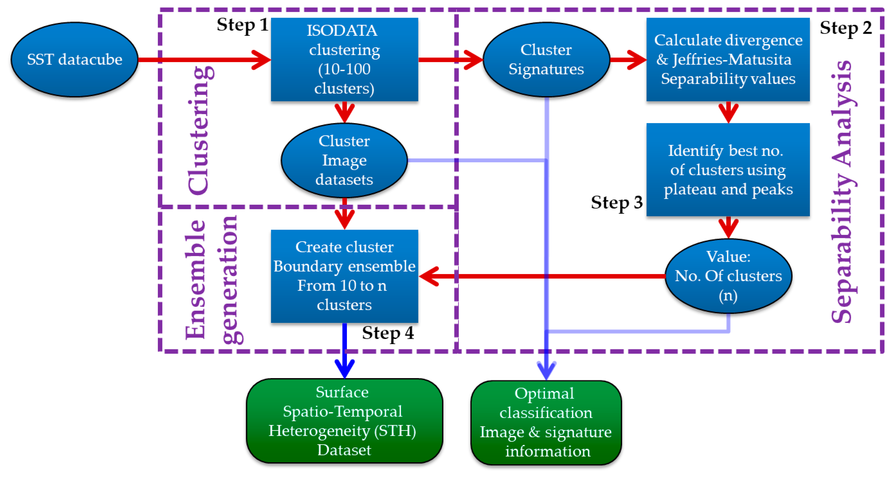
2.2.3. OHMA Implementation

The Ocean-surface Heterogeneity MApping (OHMA) process is detailed in Figure 3. It is automated once the input data are selected. Outputs include (i) a single STH dataset, (ii) an optimal cluster image dataset which best represents the variability in the data, and (iii) the temporal signatures associated with that cluster image. Steps 1 and 4 follow the LaHMa algorithm [28] and amendments noted by Ali et al. [11].

The hypertemporal SST image dataset was processed through a series of unsupervised classification runs, using an Iterative Self-Organising Data Analysis (ISODATA) approach in Erdas IMAGINE 2018 software. These were executed with each run generating a pre-defined number (from 10 to 100) of output clusters. All ISODATA clustering runs were implemented with the number of iterations set to 50, the convergence threshold set to 1.0, and zero values classified. The ISODATA runs also produced a signature file to accompany each cluster dataset, containing statistical summaries of the cluster values arranged per-image over time (signatures). For each classification, divergence and Jeffries-Matusita separability measures [35,36,37] were calculated between all possible pairs of signatures, to assess their separability. The minimum and average divergence, and Jeffries-Matusita, indices were then extracted to represent each run.

The key enhancement to the LaHMa approach is the use of the Jeffries-Matusita measure. In Erdas IMAGINE, Jeffries-Matusita distance (J_ij) is calculated as the separability of a pair of probability distributions, using the formula [35]:

$$J_{ij}=\sqrt{2\left(1-e^{-B_{ij}}\right)}$$

(1)

where:

$$B_{ij}=\frac{1}{8}{\left({\mu }_i-{\mu }_j\right)}^T{\left(\frac{C_i+C_j}{2}\right)}^{-1}\left({\mu }_i-{\mu }_j\right)+\frac{1}{2}\ln \left(\frac{\left|\frac{C_i+C_j}{2}\right|}{\sqrt{\left|C_i\right|\left|C_j\right|}}\right)$$

(2)

where:

• i and j = two temporal signatures (classes) being compared,
• C_i = the covariance matrix of signature i,
• C_j = the covariance matrix of signature j,
• µ_i = the mean vector of signature i,
• µ_j = the mean vector of signature j,
• ln denotes the natural logarithm function, and
• T denotes the transpose of a matrix.

The square root of Jeffries-Matusita, which is asymptotic towards $\sqrt{2,}$ (Equation (1)), gives a plateau at ~1.414 [35]. This plateau was exploited to remove subjectivity from the separability analysis step.

The separability data for all runs were then plotted against the number of classes generated by each run (Figure 4). The plot was interpreted objectively using pre-defined criteria, to select the optimal number of clusters to represent the variability in the processed hypertemporal SST image dataset. The pre-defined criteria were as follows:

• The number of clusters selected was the lowest number which satisfied the separability criteria;
• The cluster number selected featured a positive peak in both the minimum and average Divergence separability measure;
• The cluster number selected features a Jeffries-Matusita value of 1.414 or above (denoting the highest level of separability between all clusters [38]).

This coupling of the divergence peak-seeking approach [28,29] to an analysis of Jeffries-Matusita characteristics (Steps 2 and 3 in Figure 3) is the key aspect for ocean science applications. Only when the minimum Jeffries-Matusita separability is at 1.414 or above, are coincident peaks in divergence acceptable as indicators of the upper bounds of the OHMA cluster boundary ensemble (Figure 4). The process of optimising the number of clusters and producing the cluster ensemble is thus fully automated, without need for expert knowledge of the region, and meeting the ocean science criteria outlined in [26].

For each cluster dataset image, from 10 up to the optimal number of clusters (in this case 53 clusters), the cluster boundaries were extracted using ESRI ArcMap Version 10.5. As per the LaHMa approach [11,28], each output raster was first converted to a vector polygon, maintaining the integrity of the pixel boundaries by de-selecting the option to “simplify polygons”. These polygons were then converted into polylines, with each feature given a value of 1. The polyline file was converted to a 1/0 raster image with a pixel resolution 1/6th the spatial resolution of the original SST imagery. These 44 1/0 image datasets were then summed, to produce a single raster image with raster values from 0 to 44. The raster pixels were then aggregated using a cell factor of 6, and selecting the maximum value technique. This was the approach used by Ali et al. [11] to produce the raster STH image dataset of the same spatial resolution and spatial completeness as the input data.

The output of the process is effectively a per-pixel count of the number of cluster boundaries which lie across that pixel, over the course of an objectively defined range of classification runs. The pixel value in a STH dataset can be defined as follows:

$$ST{H}_p={\displaystyle \sum }_{n=k_l}^{k_u}{b}_{p,n}$$

(3)

where:

• b = 1, pixel (p) contains a cluster boundary,
• b = 0, pixel (p) does not contain a cluster boundary,
• STH_p = surface spatio-temporal heterogeneity in a pixel (p),
• k_u = optimal number of clusters to represent data variability, and
• k_l = lowest number of clusters to represent data variability.

Within each cluster image, these boundaries separate groups of clustered pixels, grouped on the basis of their temporal profiles statistical characteristics. Pixels with higher STH values more dependably separate regions with different parameter (in this case temperature) profiles over the analysed time period. The single-image dataset contains spatial, temporal and difference information, with the pixel values giving estimates of spatio-temporal heterogeneity (STH). A fully detailed summary of the development of the OHMA algorithm adaptations is provided in [39].

2.3. Validating the OHMA Output, with In Situ Heterogeneity Estimates

2.3.1. Research Vessel Underway Measurements of Surface Temperature

Underway data on subsurface temperatures were collected by Ireland’s Marine Institute during multiple scientific surveys over 2011. These data are freely available via Ireland’s Digital Ocean online portal [40]. Temperature measurements were taken at 3 to 6 metres depth using a thermosalinograph (Seabird, SBE21 with temperature sensor SBE38) on board the RV Celtic Explorer [41,42], and RV Celtic Voyager [43,44]. Each cruise is treated as distinct, as the sensors may have been swapped out intermittently to be calibrated. However, the heterogeneity of absolute values within individual cruises can be considered to be reliable for validating the STH values. For the purpose of this study, a transit was considered to be the sequence of temperature measurements acquired by the vessel’s thermosalinograph, while the vessel travels through the area of an STH image pixel.

2.3.2. Spatial and Temporal Bias Reduction to Derive Comparable Heterogeneity Measures

To overcome the spatial and temporal sampling bias in the in-situ transit data, a three-stage bias-reduction approach was taken. Firstly, a grid with STH pixel extents was created. Only pixel areas which featured at least one measurement in all four quarters of 2011 (Q1 = 1 January to 31 March; Q2 = 1 April to 2 July; Q3 = 3 July to 30 September; and Q4 = 1 October to 31 December) were selected as potentially acceptable validation sites. Pixels adjacent to the coastline and in close proximity to each other were discarded, to reduce (i) the influence of mixed pixels and (ii) any potential for spatial autocorrelation. Of the 3677 Underway-sampled pixels, 14 pixels had acceptable data coverage of each quarter of 2011 (Figure 5). These validation pixels all lie in the CSR around the coastline of Ireland where the Marine Institute vessels typically operate, and had STH values that ranged from 0 to 29 (excluding coastal or poor SST data artifact pixels). This compares to a range of 0 to 39 for the full STH dataset (the NAA region). Each validation pixel’s longitude and latitude is 0.102°, giving a sampling area between approximately 81.4 km² to 74.7 km², depending on latitude.

Sampling frequency, coupled with the high variability in vessel speed and area covered, increases the potential for a spatial sampling bias. In an effort to reduce this, stage two sub-divided each of the 14 selected pixels (spatial resolution ~0.102°) into a 25 × 25 grid of sub-pixels (spatial resolution 0.004°). The mean temperature of each sub-pixel was obtained, with the full pixel heterogeneity measures calculated from the sub-pixel values. In four cases, a vessel transit gathered less than five measurements across a pixel. In these cases, to maximise the number of measurements available, ten measurements before and after the research vessel crossed the adjacent pixel boundary were used. These were sub-pixellated, and averaged with the central measurements to calculate transit heterogeneity. Measures of statistical dispersion (range, h-spread, standard deviation, and variance) and of statistical shape (kurtosis, absolute kurtosis, skewness, and absolute skewness) were calculated from each pixel’s set of sub-pixels, giving a measure of its in-situ heterogeneity for the vessel transit. The cumulative difference in sequential measurements along a pixel transit, and the mean difference in sequential measurements over a pixel transit, were also calculated, as additional measures of statistical dispersion.

Bias introduced by excessive sampling during a single annual quarter, was addressed by stage three. The mean heterogeneity values of the cruises within each annual quarter were calculated. The annual mean was then derived from these four values. The final annual value is thus more spatially and temporally comparable to that pixel’s OHMA-derived STH value. A Spearman’s rank correlation analysis was then used to compare each in-situ-derived heterogeneity measure to its STH counterpart. This was seen as adequate to provide information on the STH datasets validity, noting sub-optimal sample size (14 samples). It also allowed the potential interpretation of an SST-derived STH value to be explored.

2.4. Characterising the STH Product Using Physical Phenomena

Using Generalised Linear Modelling, the 2011 STH dataset was compared to a number of modelled fronts, currents and bathymetric products generated using data from different satellite sensors, and in-situ measurements (

Table 1. Input parameters, and source datasets for STH output characterisation.

Oceanographic Measure	Source	Parameter Generated
Surface Spatio-Temporal Heterogeneity (STH)	Generated within study	STH
Sea Surface Temperature Fronts(SSTFs)	PML-generated SSTF data produced using the process outlined in [45]	(Count) No. of SSTFs
		Mean SSTF magnitude
		Median SSTF magnitude
		Standard deviation in SSTF magnitude
		Maximum SSTF magnitude
		Minimum SSTF magnitude
Sea Surface Speed (SSSp)	GlobCurrent Sea Surface Current data [46]	Mean SSSp
		Median SSSp
		Standard deviation in SSSp (StDv SSSp)
		Maximum SSSp
		Minimum SSSp
		High-pass edges in Mean SSSp
		High-pass edges in StDv SSSp
Bathymetry	GEBCO Bathymetry data [47,48]	Absolute bathymetry
		Aspect
		Slope

). The focus here was to determine if the STH features were related to physical ocean surface phenomena, and geophysical sub-surface features.

2.4.1. Datasets on the Physical Phenomena

Sea surface Temperature Front (SSTF) data were generated and provided by Plymouth Marine Laboratory as outlined in [45,49], for the NAA area. Discrete 7-day front images were generated for 2011 (1–7 January, 8–15 January, etc.) from weekly composited microwave and infrared SST data at 9 km spatial resolution. A threshold of a minimum SST step of 0.6 °C across a pixel, was used to flag and identify the presence of a thermal front in the SST imagery [50]. Note that a single-day front image for 31 December was incorporated into the dataset to match the OHMA data inputs (1 January–31 December 2011). Table 1 shows the range of statistical summaries that were derived from these SSTF images.

Modelled sea surface current data, produced under the Globcurrent initiative [46] were obtained freely from the Copernicus Marine Environment Monitoring Service (CMEMS) portal [51]. Discrete 1-day surface current images, corresponding to the OHMA input datasets (i.e., 1 January, 8 January, etc.) were subset to the NAA area. These were processed into directionless, geostrophic current speed images in ms⁻¹ at weekly intervals, and at ~0.25° spatial resolution. Table 1 presents the list of summary statistics calculated.

Bathymetry data for all four case study areas were obtained from the General Bathymetric Chart of the Oceans (GEBCO), developed through the Nippon Foundation-GEBCO Seabed 2030 project [47,48]. The GEBCO_2019 data product provides global bathymetric coverage on a 15 arc-second grid. Data values refer to elevations at the centre of each grid cell. The elevation models are generated by assimilating heterogeneous data types at mean sea level. The GEBCO grid created uses the ‘base’ Version 1 of the SRTM15+ dataset [52,53], augmented with datasets from a number of international and national data repositories and regional mapping initiatives. Three measures of the ocean floor (slope, aspect and absolute bathymetry) were derived from the GEBCO dataset (Table 1).

2.4.2. Characterisation Approach

The various statistical summary images of bathymetry, SSTF and SSSp image data were re-sampled to match the spatial resolution of the STH dataset (~0.102°), using a centroid-regridding approach. Re-sampling parameter datasets to the lowest spatial resolution dataset (SSSp), could have introduced a higher level of information loss from the SSTF dataset. With this in mind, the STH resolution was selected as it lay between that of both the lowest resolution (SSSp), and highest resolution (SSTF) products, minimising any imbalance in information loss. An area-weighted number of random sampling points were generated for each case study area independently. While the geographic coordinate system WGS84 resulted in a slight sampling bias in favour of northern latitudes, it was considered acceptable for this study. Each point was populated with the co-located STH value and the comparative parameter values. For each case study, a Generalised Linear Model (GLM) [54,55] was developed with the STH values as the dependent variable. This was done using the GGally, lme4, MuMIn, car and MAS packages in an R programming framework. A GLM enables the regression analysis of a variety of non-normal responses such as binary indicators, counts and positively valued random variables [55]. The STH distributions were examined, and determined to be non-normally distributed. For each case study, a pairwise correlation analysis of all the independent parameter variables was applied, with a threshold of 0.45. This identified potentially inter-related factors in the case study area. If inter-relations were evident, one representative factor of the inter-related group was selected for input to the case study GLM. The GLM was developed by testing all possible permutations (Dredging) of the selected variables. The most straightforward model was selected from those with the lowest Akaike Information Criterion (lowest AIC +/− 8). An over-dispersion threshold of 1.5, above which corrective action is needed to address it [56], was set to determine the success of poisson-, quasi-poisson- and negative binomial models in explaining STH variability. For all case study areas, only negative binomial-based models were acceptable according to this threshold. Full details for each GLM are available in Appendix A. Each GLM was then interpreted qualitatively, using available literature on the area.

3. Results

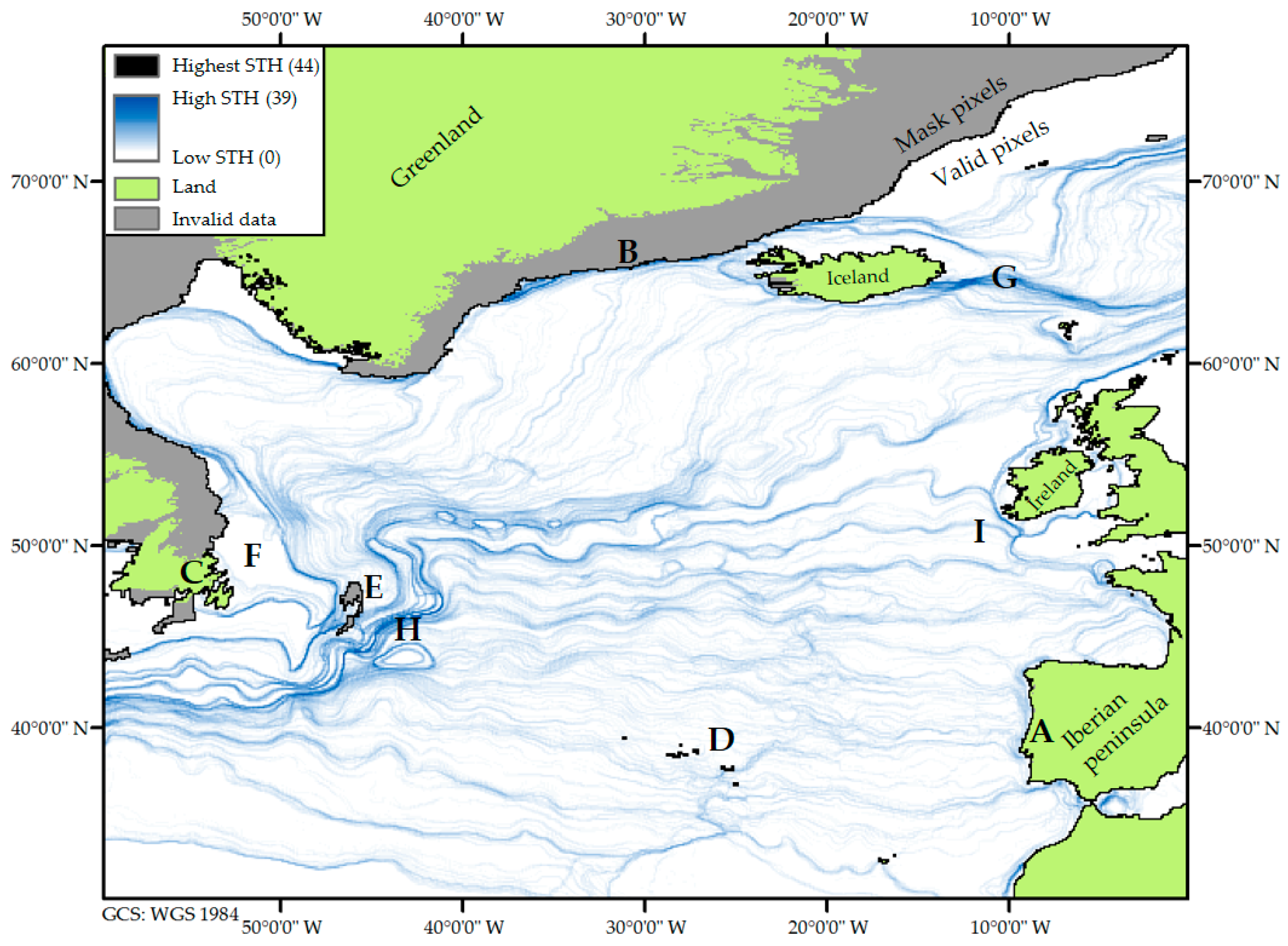
3.1. OHMA Output: A Surface Spatio-Temporal Heterogeneity (STH) Dataset

Figure 6 shows a map of the NAA region, using the surface spatio-temporal heterogeneity (STH) dataset. This dataset was generated by applying the OHMA process to a 7-day temporal resolution SST dataset for 2011. Pixels which contain a transition between valid ocean data points and mask value (land or invalid data), contained the maximum value of 44. These extreme value artifacts are highlighted as features A-E in Figure 6, and indicate the OHMA process performed as expected. Homogeneous areas, with no evidence of cluster boundaries throughout the classification runs, had a STH value of 0, (e.g., see the area east of Newfoundland, Canada represented by F in Figure 6 and examined in Figure 7a). Areas with STH values between 1 and 43 represent low to high STH, respectively. Within the valid areas, there are two extremes of STH values. An example of an area with high STH values was observed off the eastern shores of Iceland (feature G in Figure 6). Figure 7b shows this area in more detail, with a marked difference in the temporal SST signal of data pixels to the north and south of the strong elongated STH feature. Such strong STH features are evident in a number of areas across the NAA region, such as area H (Figure 6) in the vicinity of the Newfoundland Basin. Validation results, (described in Section 3.2), emphasized that higher STH pixels were associated with the presence of locally extreme values, or higher gradient transitions across adjacent areas, where there is a sudden spatial change in the surface water variable measurements. Low to medium level STH values dominate the STH map. For example, marine waters off Ireland, where in-situ data were used for validation purposes (area I in Figure 5 and Figure 6).

The OHMA process also produces (i) an image dataset of the optimal number of clusters that represent the variability in the hypertemporal datacube, and (ii) a signature file with the temporal statistical summaries of each cluster. Figure 8 highlights how cluster extent and temporal signature can be combined to produce map classes (e.g., Class 3), which can then be displayed with the STH information in a map format. As pixels are grouped by their temporal similarity, pixels in a cluster which are bounded by high STH values highlight regionally homogeneous areas, such as Class 3 in Figure 8. Figure 9 demonstrates how adjacent classes, separated by high STH values, exhibit a markedly different temporal signature from each other. High STH values separate the most temporally different regions, where more locally extreme values are encountered. This highlights the utility of the OHMA process, and the STH, cluster image and signature datasets produced. The process effectively partitions the ocean surface into regions of similarity, and regions of heterogeneity, which can be further analysed at a local level, and with additional information such as the water body characteristics at different depths.

3.2. Insights from Validating the STH Product

Correlation analysis of the 14 validation sites (data pixels) off the Irish coast determined that higher STH pixels were associated with the presence of locally extreme values, or higher gradient transitions in transit measurements acquired by research vessel. Whilst the correlations do not imply causation, they do provide evidence of potential associations. Significant associations were identified in heterogeneity measures concerned with the shape of the probability distribution of the transit temperature measurements, namely between the STH and the absolute skewness (Spearman’s Rank, n = 14, ρ[12] = +0.5755, p < 0.05), and kurtosis (Spearman’s Rank, n = 14, ρ[12] = 0.5446, p < 0.05). These shape changes can be a consequence of (i) encountering locally extreme measurement values, and/or (ii) the increased presence of sharper transitions in the transit measurements (for further information, see Appendix B). Concerning the kurtosis results, there was evidence of sampling bias, with more highly sampled pixels associated with increasingly light-tailed, platykurtic distributions (Spearman’s Rank, n = 14, ρ[12] = −0.4928, p < 0.1). There were no statistically significant associations evident between pixel STH, and in-situ (transit) heterogeneity measures classed as measures of dispersion (range, h-spread, variance, standard deviation, cumulative difference in sequential measurements, and mean cumulative difference in sequential measurements). Sampling size bias may have had an influence here, with short transits showing little dispersion in values.

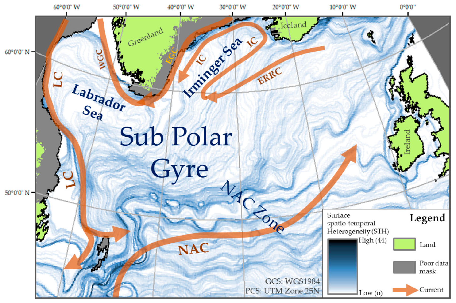
3.3. Preliminary Regional Insights from Characterising the SST STH Product

The GLM descriptions for each case study area are presented in

Table 2. Details of the Generalised Linear Models, developed to describe each of the four case study areas. Only significant effects are included in the table. Coefficients for the different variables are shown in brackets, with the level of significance indicated using asterisks. Note that SSSp = Sea Surface Current Speed, and SSTF = Sea Surface Temperature Front.

Model		Components						Performance
Case Study Area	|Bathymetry|	Slope	µSSSp	High Pass Edges in µSSSp	SSTF Count	Max SSTF Magnitude	Intercept	R2	Model Dispersion
NAA	(−7.873 × 10–5) ***		(+1.7510) ***		(+0.06118) ***	(+0.6232) ***	−0.6789	~0.2703	~1.1
NBA		(+4.832 × 10–7) ***		(+1.162) ***	(+0.04608) ***	(+0.6160) *	−0.2852	~0.3265	~1.12
CSR			(-7.676) ***		(+0.06775) ***		0.2275	~0.1719	~1.08
IFF	(−0.0004) ***	(+1.560 × 10–6) ***			(+0.06852) ***		0.4275	~0.4325	~1.09

Significance: *** p < 0.0001, * p < 0.01.

. The variability in STH was not solely explained by one factor (fronts or ocean currents or bathymetry) in any case study region. Each case study required a bespoke GLM composed of differing parameters. For the larger NAA region, factors associated with bathymetry, sea surface currents and sea surface temperature fronts explained approximately 27% of the variability evident in the STH dataset. Shallower waters were associated with higher STH values and a positive relationship was found between STH and mean sea-surface current speeds. Furthermore higher STH areas had an increased number of SST fronts, and a positive relationship with the strength of these fronts. All factors in the NAA GLM were highly significant (p-value < 0.0001; Table 2). For the NBA sub-region, approximately 32% of the STH variability could be explained by a combination of factors. The seabed gradient had a strong influence on STH values (p-value < 0.0001; Table 2). Locally higher STH areas were related to areas of higher gradient transitions in sea-surface current speeds (p-value < 0.0001; Table 2). This was also reflected in front counts (p-value < 0.0001; Table 2), and the maximum front strength to a lesser significance (p-value <0.01; Table 2). The number of detected SST fronts was also a highly significant predictor of STH values in GLMs for the CSR and IFF sub-regions. However, these two regions differed in the second influence underpinning the STH values. For the CSR, bathymetry characteristics were not good predictors of STH, and mean sea surface current speeds were negatively related to STH. In contrast, the IFF GLM showed that shallower absolute bathymetry exhibited high STH prediction, as did areas where there was an increased seabed slope. There was little or no influence of sea surface current speeds on STH values found in the IFF GLM. All factors in the CSR and IFF models were highly significant (p-value < 0.0001; Table 2), explaining approximately 17% (CSR) and 43% (IFF) of the variability in the two sub-regions.

Drawing on existing oceanographic knowledge of the North Atlantic basin, preliminary interpretation of co-located patterns in the STH dataset (heterogeneity and homogeneity features) is possible.

3.3.1. North Atlantic Area (NAA)

Two well-known features in the Atlantic Ocean include the North Atlantic’s (i) Subpolar Gyre, and (ii) Subtropical Gyre [33]. In the North Atlantic, the Subpolar Gyre is associated with a number of important overturning circulation currents, driven by changes in atmospheric forcing (winds and air–sea heat exchange). It is cyclonic in nature, and its associated boundary currents move around the North Atlantic in an anticlockwise direction. The spatio-temporal heterogeneity map (Figure 6 and Figure 8) shows higher STH values where some of the boundary currents are located (e.g., the North Atlantic Current, East Greenland and Labrador Currents shown in Figure 10). The lower part of the STH map (Figure 6 and Figure 8) shows the northern boundary of the Subtropical Gyre to the south. This demonstrates the potential in using heterogeneity features such as Earth Observation-derived fronts to reveal details of surface currents, which are not resolved by in-situ or altimetry measurements [57]. The STH dataset also shows a similar pattern to cold surface waters moving southwards in the Labrador Current. Boundaries depicted around the homogenous area F of Figure 6, and Class 3 in Figure 8, resemble the extent of the continental shelf ice-influenced pelagic habitat, identified in other ocean surface partitioning studies [4,58]

3.3.2. Newfoundland Basin Area (NBA)

Figure 11 shows an isolated ovoid STH feature in the central Newfoundland Basin. This feature is located where a semi-permanent, mesoscale (~140 km radius) anti-cyclonic eddy known as a Mann Eddy is expected [63]. The Mann Eddy, first described in 1967 [32], is located in the vicinity of the North Atlantic Current. It plays an important role in the circulation, air–sea interaction, and climatology of the region [63], and is “nearly always observed offshore of the North Atlantic Current near 42°N” [64]. However, further examination of the temporal SST development of the feature, and surrounding water classes (Figure 11), indicates the STH feature is not distinguished solely by its elevated heat expression, as would be expected if SST alone could determine this phenomenon. The cooler water period also identifies it as a surface water class. This indicates that other ocean surface processes influence the regional SST signals, and offers an opportunity to study and clarify the regions surface water dynamics.

3.3.3. Celtic Seas Region (CSR)

The STH map extending over the Celtic Seas Region (CSR) exhibits some characteristics that are similar to a number of regionally important oceanographic features. Medium-intensity STH aligns with regionally important features, such as the thermohaline driven Irish shelf front situated off the coast of Ireland [65], and the Celtic Sea front [66] that separates the Celtic Sea, from the Irish Sea, particularly during the summer months [67,68]. The STH dataset clearly separates Irish coastal waters from offshore oceanic shelf waters, as they feature distinctive temporal profiles (Figure 12, classes 21 and 24). Beaugrand et al. identified the Celtic Sea region as a biogeographic crossroads, noting that in this area, oceanic, neritic and pseudo-pelagic species cohabit, with warm- and cold-water species regularly co-occuring [58]. They highlight the potential for complex coenoclines (a gradient of associated communities), and associated ecosystems, ecoclines and ecotones to exist in the area. Similar observations were noted by Barnard et al. in their investigation into plankton communities of the North Atlantic [69].

Figure 13 shows the STH dataset overlying SSSp and SSTF counts, the two variables identified in the GLM as significant in this region. An inverse relationship between STH and surface current speed is clearly visible in the NW quadrant of Figure 13a. SSSp is regionally high over the Rockall trough, a deep underwater canyon. The STH values are low in adjacent waters, and high STH values are visible to the south (Porcupine Bank), east (Malin Shelf) and northwest (Rockall Bank). Here, the elevated STH values are associated with higher SST front counts (Figure 13b). It is notable that the strength of these many fronts was relatively weak, in comparison to those elsewhere in the North Atlantic region.

3.3.4. Iceland—Faroes Front Region (IFF)

The surface spatio-temporal heterogeneity (STH) map and key classes are used to describe the IFF region (Figure 14). Here, the GLM identified bathymetry as an important characteristic, with the highest STH values observed in shallower waters (Figure 15a). This was most pronounced in locations with steeper gradients over a short seabed distance (Figure 15b). SST Front counts, while often weak, also exerted an important influence in the GLM (see Figure 15c). The poleward flow of surface Atlantic Ocean waters across the Greenland-Scotland ridge, through the Nordic Seas, and into the Arctic Ocean plays a fundamental part in ocean heat transport and thermohaline circulation in the region [70]. Approximately 50% of warm-saline surface inflows [70] of modified North Atlantic water into the Nordic Seas follows a path between Iceland and the Faroe Islands. In this dynamic region, the surface warm saline Atlantic water meets colder, less saline waters. This confluence of different water types is marked by the Icelandic—Faroe Front [71,72,73]. To the east, the Faroe Shelf Front [74,75] marks the region where the Atlantic waters meet tidally well-mixed waters on the Faroe shelf. Both these boundary regions were highlighted remarkably well by high STH values in this study (Figure 14). Furthermore, bathymetric and shelf influences on these surface to bottom frontal systems were also captured in the GLM for the region. This echoes the findings of some hydrographic frontal studies, where a general dependence of frontal locations on bathymetry was noted [71]. The IFF area is a key example of why the study of surface spatio-temporal heterogeneity needs to consider the influence of sea bed topography on the surface behaviour. Interpretation of a STH dataset requires the researcher to understand the ocean as a four dimensional system, with processes and features at the ocean depths influencing the ocean surface signals to differing degrees over time.

4. Discussion

The OHMA method to map ocean surface spatio-temporal heterogeneity is a data-driven, unbiased approach, which exploits the hypertemporal resource of remote sensing-derived datasets. It successfully adapts the LaHMa method [28] for use in ocean sciences. The addition of a Jeffries-Matusita analysis step enables the entire process to be automated, and executed without prior knowledge of the region under examination.

The use of OHMA can enhance efforts to understand the regional structure of the ocean surface. It is known that the ocean surface can be organised into regions with distinct abiotic and biotic properties, that change over space and time [76]. One approach to understanding this surface diversity (heterogeneity), is Ocean Surface Partitioning (OSP) [4,58]. OSP aims to effectively group areas of the ocean surface together into delineated ocean ‘provinces’. It is increasingly seen as an approach to help understand the patterns of ocean spatio-temporal variability [77], and the impacts of this variability [78]. Krug et al. give an extensive insight into the range of OSP methodologies and applications available [76]. More recently, there has been discussion on the benefits of enhancing static outputs (e.g., those of [4], and [58]) with more dynamic outputs (e.g., [77,79,80]). There is also discussion concerning the range of datasets which can be input to a partitioning strategy [58], and whether abiotic parameters, biotic parameters, or both, should be used to define provinces [4,58,77,81].

Whilst these discussions continue, there are opportunities to advance different perspectives on partitioning the ocean surface. Currently, OSP is inherently reliant on the grouping of ocean surface areas into coherent, well-defined and bounded areas of similarity. These areas can then be described using the input parameters, e.g., through defining ecosystem partitions [77], biological partitions [78], biogeographical partitions of varying complexities [4,58], or even phenological metrics [81]. These partitions rely on classification, effectively grouping homogeneous regions together and delineating their extents. Less obviously stated, is that by grouping areas together, we highlight their difference from other areas, and the nature of transitions between them. However, there is limited consideration of the influence of sharper spatio-temporal transitions in regional abiotic properties, and their impact on regions of increased photosynthetic activity. The STH information produced using the OHMA process could be particularly supportive as an input to OSP classification approaches. This is especially relevant given this research has shown that the OHMA-derived STH data product is a hybrid product, capturing several aspects of heterogeneity in a single measure.

Furthermore, there is an opportunity to explore whether the biological characteristics of a region are underpinned by a transition in abiotic conditions within it. In this study, the mapped, SST-based heterogeneity features aligned with known bio-geographical boundaries highlighted previously by Ocean Surface Partitioning (OSP) studies [4,58,79]. Areas which feature higher STH values can be considered as more permanent and/or stronger water mass boundary areas. Conversely, weaker STH values indicate regions where boundaries are weaker and/or more mobile and transitory over space and time.

This fluid, impermanent nature of ocean boundaries highlights a further opportunity. Multiple authors have noted the limitations of adopting purely static approaches to OSP [79,80]. Instead they adopted more dynamic methods to delineate provinces. These have consistently enhanced the delineation of biogeochemical province boundaries, while producing a number of maps to chart changes over seasons and years. The STH mapping proposed here can support such efforts. It offers insights into the characteristic permanence of statically mapped boundaries, on the basis of the input parameter. As such, pre-examination of a region using an OHMA approach could help objectively determine whether or not a more dynamic methodology is required.

The validation efforts highlighted a gap in in-situ data availability. 14 pixels were available with a sufficient temporal sampling quality to be comparable to the temporally rich satellite-derived SST dataset. While the associations between STH and in-situ skewness and kurtosis could be clarified, the sampling volume was not sufficient to properly examine the measures of dispersion. From the in-situ perspective, this information is only available for 14 pixel locations in Irish coastal waters, for a dataset spanning the North Atlantic. It involved processing an entire year of all available cruise data from two vessels, to extract temporally comparable measures to the satellite-derived product. As such, it is not currently feasible, using only in-situ data, to produce surface spatio-temporal heterogeneity maps at the spatial and temporal scales offered by OHMA. This not only emphasized the potential for STH datasets to complement existing efforts, it also demonstrated an observation gap at the in-situ level, which could be addressed. In addition to the Underway data collected by the Marine Institute [41,43], there are a number of examples of in-situ measurements being taken in transit and made available (for example data available through the GOSUD initiative [82], and the Shipborne-radiometer Network [83]). The challenging nature of the validation work highlighted the need to establish a set of dedicated spatio-temporal validation sites specifically measured using vessel transits. There is an opportunity for the ocean remote sensing community, and in-situ ocean observing community to identify key areas to sample, and direct vessels through. Establishing these sites would help to fully unlock the potential of hypertemporal data archives, and spatio-temporal data products.

The GLM element of this study was preliminary in nature, seeking to place the STH product in terms of available, recognised heterogeneity products. The multi-factor models, with highly significant, though low, R² values emphasized that (i) regional surface water heterogeneity was driven by a range of factors, and (ii) there remains unidentified drivers of surface water STH, far beyond what is typically used (fronts, currents and bathymetry). Future work would be well advised to introduce a number of other parameters to the regional models, such as Sea Surface Salinity [84], or altimetry-derived sea level products ([85]) for example. In particular Sea Surface Salinity and sea level products would be well positioned to factor into GLM models for open ocean-focused studies, given their good performance in waters that are further offshore [84,85,86]. Other modelled parameters such as mixed-layer depth could also be considered if available.

In spite of its preliminary nature, the GLM study demonstrated the hybrid nature of the STH dataset. It captured different aspects of heterogeneity at the NAA scale, and in each different case study sub-region, yet delivers the information as a single measure. As such, the unique nature of the STH product was highlighted, as was its potential to serve as a single heterogeneity measure to support biodiversity and habitat mapping. Further work on multi-parameter studies investigating both the physical and biotic environment could be conducted using OHMA-derived STH datasets. This could clarify whether (i) the same logic applies across parameters, and (ii) whether STH datasets can enhance our understanding of biophysical systems in ocean surface waters.

Such systemic studies of the ocean surface need to be founded on understandings of regional oceanographic characteristics and features. This study demonstrated the utility of STH mapping to support such work. STH datasets, in combination with their ancillary classification datasets, reveal surface units which share high strength boundaries. These oceanic ecotones with pronounced gradient changes over small spatial scales, are evident in the NBA and IFF regions (shown as features G and H in Figure 6). These areas feature well studied frontal systems, co-located with high STH values. The high STH values highlight regions with greater mixing of water masses, potentially greater per-unit area diversity in habitat niches over time, and the presence of high-gradient transitions which can be exploited by species (for example Tuna species [18,87]), and thereby shape their distributions.

Meanwhile, contrasting this are surface units which do not share high, or even medium strength boundaries. These oceanic ecoclines (such as F in Figure 6), are regions across which the temperature profiles of the surface waters change, but gradually over spatial scales, without clear separable persistent boundaries between the surface water classes. These ecoclines are potentially useful. Their surrounding boundaries potentially delineate extensive regions, across which surface conditions and temporal fluctuations change gradually. The direction of change is indicated by both the mapped ecotones and ecoclines, coupled with the surface water class locations. Use of regular, persistent features and their spatial locations could be useful in targeting in-situ surface water studies specifically looking at change. It offers the potential to objectively chart sampling transects to capture the spatio temporal gradients, and enhance the cost–benefit ratio of ocean-going research cruises measuring them. These bounded ecoclines are also useful for the ocean remote sensing community, in particular those conducting time-series analyses on remotely sensed data. Time-series analysis can be used to explain and characterise the occurrence of observed temporal phenomena [88]. However, its use in ocean studies is restricted by the need for experience, and a-priori knowledge of regional seasonalities [26], used to guide model training [89]. Here, the suite of OHMA output datasets could be of use. The STH boundaries, classification maps and temporal legends can provide insights into the diversity of temporal signals the modeler must account for. The suite can also be used to define the larger more homogeneous regions for temporal sampling, particularly when seeking to define the endmembers needed for Temporal Mixture Analyses [90]. As such the objective nature of the OHMA process enhances the opportunities for these more restricted approaches to be deployed. This objective capability to quantify natural mobile discontinuities (ecoclines), and continuities (ecotones), also shows the approach could support the development of seascape [91] characterisations. Such applications have already been demonstrated in terrestrial landscape studies [11,28], noting that Kavanaugh et al. emphasize the need to characterise planktonic processes in support of seascape characterisations [91].

The methodology also captured information on a range of oceanographic features, which are difficult to measure at large spatial scales using in-situ measurements alone. Features such as the boundaries and meanders of the Gulf Stream at the surface (Figure 8), the Mann Eddy (Figure 11), the Celtic Sea Front (Figure 12), and the Icelandic and Faroes fronts (Figure 14 and Figure 15), are a range of globally, and/or regionally important macro- to mesoscale oceanic features, which are identifiably delineated by the STH dataset. It demonstrated the ability of the OHMA process to objectively quantify the spatial extents of these features, over a given timeframe, and gain a measure of their regional significance. A further step could see these features examined using more regionalised, and higher spatial and temporal resolution datasets. This could maximise their influence on the clustering process, and potentially better delineate them, and their spatio-temporal relevance. However, there would also be the risk that regionally, these features are not as distinctive as they are globally. Furthermore, as found by de Bie et al. when examining the Mekong Delta using the LaHMa method [28], higher spatial resolution imagery can misrepresent the diversity of the surface. In the Mekong study, this resulted in landscape-level gradient information being obscured beneath anthropogenic rural and urban boundaries. It remains to be seen whether deploying OHMA on finer spatial resolution data, will suffer from the same issues, given the lack of anthropogenic structures on the ocean surface.

Finally, it is unclear whether the OHMA process can adequately capture the temporal development of ocean surface features. Evidence from this study suggests that features such as near-surface currents in the Gulf Stream system, the Mann Eddy, and certain frontal systems (Figure 6, Figure 10, Figure 11 and Figure 15) leave a signature in the measured SST image data, which can be highlighted and enhanced by the OHMA process. This could serve to highlight regions for further investigation, whereupon sea surface temperature front data could be generated using [49,50], or time-series of current characteristics could be generated using [92]. Alternatively shorter timeframes of more regionalised data could be input to generate OHMA-derived STH datasets. However, it remains unexplored whether the use of shorter temporal extents better delineate, or miss these features, and indeed, how the researcher should approach using OHMA to study features with a more rapid spatio-temporal character, such as fast moving mesoscale eddies. From the opposing perspective, the temporal stability of features could be examined. Some archives of SST now span climatological timeframes. This offers the potential to map and monitor more permanent ocean STH structures, quantify their temporal behaviour over climatological timeframes, and begin monitoring their stability as more heat energy circulates through Earth’s systems.

5. Conclusions

The OHMA methodology is a robust tool suitable for the ocean science community to explore, examine, and describe the ocean’s surface. It produces an objective higher-level heterogeneity product, which summarises information from hypertemporal image data, and successfully captures a range of ocean-surface heterogeneity perspectives (such as fronts, currents, and locally extreme values). In doing so, it advances our capability to map ocean surface spatio-temporal heterogeneity, with the potential to provide information on biophysical processes which affect the distribution of marine species.

Similar to the LaHMa method, the output STH dataset captures and presents oceanic ecotones and ecoclines, particularly when viewed alongside the ancillary classification dataset and legend which are produced as part of the process. In doing so, it enables us to objectively map regions of spatio-temporal change. This study described and demonstrated the validity, and potential utility, of this adapted STH mapping algorithm for ocean sciences, tailored to exploit hypertemporal Earth Observation imagery. Validation efforts indicate the algorithm detects locally increased transitions in the input ocean surface parameter (here demonstrated using SST). Characterisation using a range of ocean parameters showed the OHMA approach provides a high-level perspective of ocean surface heterogeneity. This enables the identification of high-change regions, and subsequent exploration using other measured/modelled parameters, or more targeted site investigations. Using hypertemporal SST imagery as an input, the algorithm proved effective at highlighting areas of increased SST front frequency, indicators of boundaries between water masses. Perspectives on surface currents and the underlying bathymetry were also related, to differing degrees, and in different combinations, to STH in the suite of case study areas. A number of future avenues for work were highlighted including (i) using regional coastal studies to examine the performance of the algorithm in more complex scenarios, (ii) examining the algorithm performance on a range of datasets at different temporal and spatial scales, and (iii) exploring ocean surface systems using STH products derived from a range of ocean surface parameters. The study also highlighted the need to establish dedicated spatio-temporal ocean validation sites, specifically measured using surface transits, to support advances in hypertemporal ocean data use, and exploitation.

References

1. Chesson, P.L.; Case, T.J. Overview: Non-equilibrium community theories; chance variability, history and coexistence. In Community Ecology; Diamond, J., Case, T.J., Eds.; Harper and Row: New York, NY, USA, 1986; pp. 229–239. [Google Scholar]
2. Li, H.; Reynolds, J.F. On definition and quantification of heterogeneity. Oikos 1995, 73, 280–284. [Google Scholar] [CrossRef]
3. Pianka, E.R. Evolutionary Ecology, 5th ed.; Harper Collins College Publishers: New York, NY, USA, 1994; ISBN 0065012259. [Google Scholar]
4. Longhurst, A. Ecological Geography of the Sea, 2nd ed.; Associated Press: Amsterdam, The Netherlands, 2007; ISBN 978-0-1245-5521-1. [Google Scholar]
5. Miller, P.I.; Christodoulou, S. Frequent locations of oceanic fronts as an indicator of pelagic diversity: Application to marine protected areas and renewables. Mar. Policy 2014, 45, 318–329. [Google Scholar] [CrossRef] [Green Version]
6. Brandini, F.P.; Tura, P.M.; Santos, P.P.G.M. Ecosystem responses to biogeochemical fronts in the South Brazil Bight. Prog. Oceanogr. 2018, 164, 52–62. [Google Scholar] [CrossRef]
7. Smith, R.S.; Johnston, E.L.; Clark, G.F. The role of habitat complexity in community development is mediated by resource availability. PLoS ONE 2014, 9, e102920. [Google Scholar] [CrossRef] [PubMed] [Green Version]
8. Godbold, J.A.; Bulling, M.T.; Solan, M. Habitat structure mediates biodiversity effects on ecosystem properties. Proc. R. Soc. B 2011, 278, 2510–2518. [Google Scholar] [CrossRef] [PubMed] [Green Version]
9. Isbell, F.; Craven, D.; Connolly, J.; Loreau, M.; Schmid, B.; Beierkuhnlein, C.; Bezemer, T.M.; Bonin, C.; Bruelheide, H.; De Luca, E.; et al. Biodiversity increases the resistance of ecosystem productivity to climate extremes. Nature 2015, 526, 574–577. [Google Scholar] [CrossRef]
10. Oliver, T.H.; Heard, M.S.; Isaac, N.J.B.; Roy, D.B.; Procter, D.; Eigenbrod, F.; Freckleton, R.; Hector, A.; Orme, C.D.L.; Petchey, O.L.; et al. Biodiversity and resilience of ecosystem functions. Trends Ecol. Evol. 2015, 30, 673–684. [Google Scholar] [CrossRef] [Green Version]
11. Ali, A.; de Bie, C.A.J.M.; Skidmore, A.K.; Scarrott, R.G.; Lymberakis, P. Mapping the heterogeneity of natural and semi-natural landscapes. Int. J. Appl. Earth Obs. Geoinf. 2014, 26, 176–183. [Google Scholar] [CrossRef]
12. Gratwicke, B.; Speight, M.R. The relationship between fish species richness, abundance and habitat complexity in a range of shallow tropical marine habitats. J. Fish Biol. 2005, 66, 650–667. [Google Scholar] [CrossRef]
13. Margalef, R. Our Biosphere; Inter-Research: Oldendorf, Germany, 1997; ISBN 0-932-2205. [Google Scholar]
14. Longhurst, A. Fronts and pycnoclines: Ecological discontinuities. In Ecological Geography of the Sea; Longhurst, A., Ed.; Associated Press: Amsterdam, The Netherlands, 2007; pp. 35–50. ISBN 978-0-1245-5521-1. [Google Scholar]
15. Scales, K.L.; Miller, P.I.; Hawkes, L.A.; Ingram, S.N.; Sims, D.W.; Votier, S.C. On the front line: Frontal zones as priority at-sea conservation areas for mobile marine vertebrates. J. R. Soc. Interface 2014, 11, 1–9. [Google Scholar] [CrossRef] [Green Version]
16. Bakun, A. Fronts and eddies as key structures in the habitat of marine fish larvae: Opportunity, adaptive response and competitive advantage. Sci. Mar. 2006, 70, 105–122. [Google Scholar] [CrossRef]
17. Schmid, M.S.; Cowen, R.K.; Robinson, K.; Luo, J.Y.; Briseño-Avena, C.; Sponaugle, S. Prey and predator overlap at the edge of a mesoscale eddy: Fine-scale, in-situ distributions to inform our understanding of oceanographic processes. Sci. Rep. 2020, 10, 1–16. [Google Scholar] [CrossRef] [Green Version]
18. Xu, Y.; Nieto, K.; Teo, S.L.H.; McClatchie, S.; Holmes, J. Influence of fronts on the spatial distribution of albacore tuna (Thunnus alalunga) in the Northeast Pacific over the past 30 years (1982–2011). Prog. Oceanogr. 2017, 150, 72–78. [Google Scholar] [CrossRef]
19. Santos, A.M.P.; Kazmin, A.S.; Peliz, Á. Decadal changes in the Canary upwelling system as revealed by satellite observations: Their impact on productivity. J. Mar. Res. 2005, 63, 359–379. [Google Scholar] [CrossRef]
20. Kimura, S.; Nakata, H.; Okazaki, Y. Biological production in meso-scale eddies caused by frontal disturbances of the Kuroshio Extension. ICES J. Mar. Sci. 2000, 57, 133–142. [Google Scholar] [CrossRef]
21. Lee, T.N.; Yoder, J.A.; Atkinson, L.P. Gulf Stream frontal eddy influence on productivity of the southeast US Continental Shelf. J. Geophys. Res. 1991, 96, 191–205. [Google Scholar]
22. Nygård, H.; Oinonen, S.; Hällfors, H.A.; Lehtiniemi, M.; Rantajärvi, E.; Uusitalo, L. Price vs. value of marine monitoring. Front. Mar. Sci. 2016, 3, 1–11. [Google Scholar] [CrossRef] [Green Version]
23. Klemas, V. Fisheries applications of remote sensing: An overview. Fish. Res. 2013, 148, 124–136. [Google Scholar] [CrossRef]
24. Stuart, V.; Platt, T.; Sathyendranath, S.; Pravin, P. Remote sensing and fisheries: An introduction. ICES J. Mar. Sci. 2011, 68, 639–641. [Google Scholar] [CrossRef]
25. Piwowar, J.M.; Wessel, G.R.I.; LeDrew, E.F. Image time series analysis of Arctic sea ice. In Proceedings of the Geoscience and Remote Sensing Symposium; IGARSS ’96. “Remote Sensing for a Sustainable Future. IEEE: Lincoln, NE, USA, 1996; pp. 645–647. [Google Scholar]
26. Scarrott, R.G.; Cawkwell, F.; Jessopp, M.; O’Rourke, E.; Cusack, C.; de Bie, K. From land to sea, a review of hypertemporal remote sensing advances to support ocean surface science. Water 2019, 11, 2286. [Google Scholar] [CrossRef] [Green Version]
27. Kleynhans, W. Detecting Land-Cover Change Using MODIS Time-Series Data; University of Pretoria: Pretoria, South Africa, 2011. [Google Scholar]
28. de Bie, C.A.J.M.; Nguyen, T.T.H.; Ali, A.; Scarrott, R.; Skidmore, A.K. LaHMa: A landscape heterogeneity mapping method using hyper-temporal datasets. Int. J. Geogr. Inf. Sci. 2012, 26, 1–16. [Google Scholar] [CrossRef]
29. de Bie, C.A.J.M.; Khan, R.; Toxopeus, A.G.; Venus, V.; Skidmore, A.K. Hypertemporal image analysis for crop mapping and change detection. In Proceedings of the The International Archives of the Photogrammetry, Remote Sensing and Spatial Information Sciences; Volume XXXVII. Part B7. Beijing 2008. International Society of Photogrammetry and Remote Sensing: Beijing, China, 2008; Volume 2, pp. 803–814. [Google Scholar]
30. Nguyen, T.T.H.; de Bie, C.A.J.M.; Ali, A.; Smaling, E.M.A.; Chu, T.H. Mapping the irrigated rice cropping patterns of the Mekong delta, Vietnam, through hyper-temporal spot NDVI image analysis. Int. J. Remote Sens. 2012, 33, 415–434. [Google Scholar] [CrossRef]
31. Vincent, C.; Bryère, P.; Rufino, M.; Gaspar, M.; Santos, M.; Garrido, S.; Moreno, O.; Morales, J.; Duque, R.; Martinez, I.; et al. SAFI D10.2: Report on Indicators for Fishery and Aquaculture; EC: Brussels, Belgium, 2016. [Google Scholar]
32. Mann, C.R. The termination of the Gulf Stream and the beginning of the North Atlantic Current. Deep. Res. 1967, 14, 337–359. [Google Scholar] [CrossRef]
33. Talley, L.; Pickard, G.; Emery, W.; Swift, J. Atlantic Ocean. In Descriptive Physical Oceanography; Talley, L., Pickard, G., Emery, W., Swift, J., Eds.; Academic Press: Amsterdam, The Netherlands, 2011; pp. 245–301. ISBN 978-0-7506-4552-2. [Google Scholar]
34. PODAAC. GHRSST Level 4 MUR Global Foundation Sea Surface Temperature Analysis product. Version 2.0. Available online: https://podaac.jpl.nasa.gov/dataset/JPL-L4UHfnd-GLOB-MUR (accessed on 20 September 2018).
35. Pouncy, R.; Swanson, K.; Hart, K. ERDAS Field Guide, 5th ed.; ERDAS Incorporated: Atlanta, GA, USA, 1999. [Google Scholar]
36. Swain, P.H.; Davis, S.M. Remote sensing: The quantitative approach; McGraw-Hill International Book Company: New York, NY, USA, 1978; ISBN 9780070625761. [Google Scholar]
37. Richards, J.A.; Jia, X. Remote Sensing Digital Image Analysis: An Introduction, 4th ed.; Springer: Berlin/Heidelberg, Germany, 2006; ISBN 3540251286. [Google Scholar]
38. Ai, J.; Chen, W.; Chen, L. Spectral discrimination of an invasive species (Spartina alterniflora) in Min River wetland using field spectrometry. In Proceedings of the International Symposium on Photoelectronic Detection and Imaging 2013: Laser Communication Technologies and Systems, Beijing, China, 25–27 June 2013; Volume 8910, p. 89100. [Google Scholar]
39. Scarrott, R.G. Annex 2: The revised hyper-temporal processing algorithm. In H2020-CoReSyF 3rd Periodic Technical Report: Part B; Panda, K., Ed.; European Commission: Brussels, Belgium, 2019; pp. 48–63. [Google Scholar]
40. Marine Institute. Marine Data Centre. Available online: https://www.marine.ie/Home/site-area/data-services/marine-data-centre (accessed on 23 December 2019).
41. Marine Institute. Celtic Explorer Underway. Available online: https://data.gov.ie/dataset/celtic-explorer-underway (accessed on 8 December 2020).
42. Marine Institute. National Research Vessel: Celtic Explorer. Available online: https://www.marine.ie/Home/sites/default/files/MIFiles/Docs/ResearchVessels/MI-210sq-Tech Spec CE-Update 2015 FINAL.pdf (accessed on 8 December 2020).
43. Marine Institute. Celtic Voyager Underway. Available online: https://data.gov.ie/dataset/celtic-voyager-underway (accessed on 8 December 2020).
44. Marine Institute. National Research Vessel: Celtic Voyager. Available online: https://www.marine.ie/Home/sites/default/files/MIFiles/Docs/ResearchVessels/MI-210sq-CV Tech Spec 2015 FINAL.pdf (accessed on 8 December 2020).
45. Miller, P. Composite front maps for improved visibility of dynamic sea-surface features on cloudy SeaWiFS and AVHRR data. J. Mar. Syst. 2009, 78, 327–336. [Google Scholar] [CrossRef] [Green Version]
46. Rio, M.-H.; Johannessen, J.; Donlon, C. GlobCurrent Product Data Handbook: L4 Geostrophic Currents, Version 2. 0 2015, 1–30. [Google Scholar]
47. GEBCO Compilation Group. GEBCO 2019 Grid. 2019. Available online: https://www.gebco.net/data_and_products/gridded_bathymetry_data/gebco_2019/gebco_2019_info.html (accessed on 24 March 2021). [CrossRef]
48. GEBCO. General Balthymetric Chart of the Oceans. Available online: www.gebco.net (accessed on 1 May 2020).
49. Miller, P.I. Detection and Visualisation of Oceanic Fronts. In Handbook of Satellite Remote Sensing Image Interpretation: Applications for Marine Living Resources Conservation and Management; Morales, J., Stuart, V., Platt, T., Sathyendranath, S., Eds.; EU-PRESPO and IOCCG: Dartmouth, NS, Canada, 2011; pp. 229–239. [Google Scholar]
50. Miller, P.; Plymouth Marine Laboratory, Plymouth, UK; Scarrott, R.G.; University College Cork, Cork, Ireland. Personal communication, UCC-PML P.O. 10286898. 2018.
51. CMEMS Copernicus Marine Environment Monitoring Service. Available online: http://marine.copernicus.eu/ (accessed on 23 December 2019).
52. Olsen, C.J.; Becker, J.J.; Sandwell, D.T. A new global bathymetry map at 15 arcsecond resolution for resolving seafloor fabric: SRTM15_PLUS. In Proceedings of the AGU Fall Meeting Abstracts, San Francisco, CA, USA, 15–19 December 2014; p. OS34A-03. [Google Scholar]
53. Olsen, C.J.; Becker, J.J.; Sandwell, D.T. SRTM15_PLUS: Data Fusion of Shuttle Radar Topography Mission (SRTM) Land Topography with Measured and Estimated Seafloor Topography (NCEI Accession 0150537); Version 1.1; NOAA National Centers for Environmental Information: Asheville, NC, USA, 2016. [Google Scholar]
54. McCulloch, C.E. Generalized Linear Models. J. Am. Stat. Assoc. 2000, 95, 1320–1324. [Google Scholar] [CrossRef]
55. Neuhaus, J.; McCulloch, C. Generalized linear models. WIREs Comput. Stat. 2011, 3, 407–413. [Google Scholar] [CrossRef] [Green Version]
56. Zuur, A.F.; Ieno, E.N.; Walker, N.; Saveliev, A.A.; Smith, G.M. GLM and GAM for Count Data. In Mixed Effects Models and Extensions in Ecology with R; Statistics for Biology and Health; Zuur, A.F., Ieno, E.N., Walker, N., Saveliev, A.A., Smith, G.M., Eds.; Springer: New York, NY, USA, 2009; pp. 209–238. ISBN 978-0-387-87457-9. [Google Scholar]
57. Miller, P.I.; Read, J.F.; Dale, A.C. Thermal front variability along the North Atlantic Current observed using microwave and infrared satellite data. Deep. Res. Part II 2013, 98, 244–256. [Google Scholar] [CrossRef] [Green Version]
58. Beaugrand, G.; Edwards, M.; Hélaouët, P. An ecological partition of the Atlantic Ocean and its adjacent seas. Prog. Oceanogr. 2019, 173, 86–102. [Google Scholar] [CrossRef]
59. Repschläger, J.; Garbe-Schönberg, D.; Weinelt, M.; Schneider, R. Holocene evolution of the North Atlantic subsurface transport. Clim. Past 2017, 13, 333–344. [Google Scholar] [CrossRef] [Green Version]
60. Taboada, F.G.; Anadón, R. Patterns of change in sea surface temperature in the North Atlantic during the last three decades: Beyond mean trends. Clim. Chang. 2012, 115, 419–431. [Google Scholar] [CrossRef]
61. Holliday, N.P.; Bersch, M.; Berx, B.; Cha, L.; Cunningham, S.; Florindo-lópez, C.; Hátún, H.; Johns, W.; Josey, S.A.; Larsen, K.M.H.; et al. Ocean circulation causes the largest freshening event for 120 years in eastern subpolar North Atlantic. Nat. Commun. 2020, 11, 1–15. [Google Scholar] [CrossRef]
62. Koman, G.; Johns, W.E.; Houk, A. Transport and Evolution of the East Reykjanes Ridge Current. J. Geophys. Res. Ocean. 2020, 125. [Google Scholar] [CrossRef]
63. Yashayaev, I.M. 12-Year Hydrographic Survey of the Newfoundland Basin: Seasonal Cycle and Interannual Variability of Water Masses. ICES 2000, 2000, 1–17. [Google Scholar]
64. Meinen, C.S. Structure of the North Atlantic Current in stream-coordinates and the circulation in the Newfoundland basin. Deep. Res. Part I Oceanogr. Res. Pap. 2001, 48, 1553–1580. [Google Scholar] [CrossRef]
65. Huang, W.G.; Cracknell, A.P.; Vaughan, R.A.; Davies, P.A. A satellite and field view of the Irish Shelf front. Cont. Shelf Res. 1991, 11, 543–562. [Google Scholar] [CrossRef]
66. Simpson, J.H. A boundary front in the summer regime of the Celtic Sea. Estuar. Coast. Mar. Sci. 1976, 4, 71–81. [Google Scholar] [CrossRef]
67. Wang, D.P.; Chen, D.; Sherwin, T.J. Coupling between mixing and advection in a shallow sea front. Cont. Shelf Res. 1990, 10, 123–136. [Google Scholar] [CrossRef]
68. Pingree, R.D. Physical Oceanography of the Celtic Sea and English Channel. In The North-West European Shelf Seas: The Sea Bed and the Sea in Motion II. Physical and Chemical Oceanography and Physical Resources; Banner, F.T., Collins, M.B., Massie, K.S., Eds.; Elsevier: Amsterdam, The Netherlands, 1980; Volume 24, pp. 415–465. [Google Scholar]
69. Barnard, R.; Batten, S.D.; Beaugrand, G.; Buckland, C.; Conway, D.V.P.; Edwards, M.; Finlayson, J.; Gregory, L.W.; Halliday, N.C.; John, A.W.G.; et al. Continuous plankton records: Plankton Atlas of the north Atlantic Ocean 1958–1999: Preface. Mar. Ecol. Prog. Ser. 2004, 11–75. [Google Scholar]
70. Hansen, B.; Osterhus, S.; Turrell, W.R.; Jónsson, S.; Valdimarsson, H.; Hátún, H.; Olsen, S.M. The inflow of Atlantic water, heat, and salt to the Nordic Seas across the Greenland-Scotland Ridge. In Arctic-Subarctic Ocean Fluxes: Defining the Role of the Northern Seas in Climate; Dickson, R.R., Meincke, J., Rhines, P., Eds.; Springer: Dordrecht, The Netherlands, 2008; pp. 15–43. ISBN 9781402067730. [Google Scholar]
71. Smart, J.H. Spatial variability of major frontal systems in the North Atlantic-Norwegian Sea area: 1980-81. J. Phys. Oceanogr. 1984, 14, 185–192. [Google Scholar] [CrossRef] [Green Version]
72. Pistek, P.; Johnson, D.R. A study of the Iceland-Faeroe Front using GEOSAT altimetry and current-following drifters. Deep. Res. 1992, 39, 2029–2051. [Google Scholar] [CrossRef] [Green Version]
73. Tokmakian, R. The Iceland-Faroe Front: A synergistic study of hydrogaphy and altimetry. J. Phys. Oceanogr. 1994, 24, 2245–2262. [Google Scholar] [CrossRef]
74. Larsen, K.M.H.; Hansen, B.; Svendsen, H. The Faroe Shelf Front: Properties and exchange. J. Mar. Syst. 2009, 78, 9–17. [Google Scholar] [CrossRef]
75. Eliasen, S.K.; Hátún, H.; Larsen, K.M.H.; Jacobsen, S. Faroe shelf bloom phenology—The importance of ocean-to-shelf silicate fluxes. Cont. Shelf Res. 2017, 143, 43–53. [Google Scholar] [CrossRef]
76. Krug, L.A.; Platt, T.; Sathyendranath, S.; Barbosa, A.B. Ocean surface partitioning strategies using ocean colour remote sensing: A review. Prog. Oceanogr. 2017, 155, 41–53. [Google Scholar] [CrossRef]
77. Krug, L.A.; Platt, T.; Barbosa, A.B. Delineation of ocean surface provinces over a complex marine domain (off SW Iberia): An objective abiotic-based approach. Reg. Stud. Mar. Sci. 2018, 18, 80–96. [Google Scholar] [CrossRef]
78. Krug, L.A.; Platt, T.; Sathyendranath, S.; Barbosa, A.B. Unravelling region-specific environmental drivers of phytoplankton across a complex marine domain (off SW Iberia). Remote Sens. Environ. 2017, 203, 162–184. [Google Scholar] [CrossRef]
79. Devred, E.; Sathyendranath, S.; Platt, T. Delineation of ecological provinces using ocean colour radiometry. Mar. Ecol. Prog. Ser. 2007, 346, 1–13. [Google Scholar] [CrossRef]
80. Reygondeau, G.; Longhurst, A.; Martinez, E.; Beaugrand, G.; Antoine, D.; Maury, O. Dynamic biogeochemical provinces in the global ocean. Global Biogeochem. Cycles 2013, 27, 1046–1058. [Google Scholar] [CrossRef] [Green Version]
81. Krug, L.A.; Platt, T.; Sathyendranath, S.; Barbosa, A.B. Patterns and drivers of phytoplankton phenology off SW Iberia: A phenoregion based perspective. Prog. Oceanogr. 2018, 165, 233–256. [Google Scholar] [CrossRef]
82. Gosud Global Ocean Surface Underway Data. Available online: https://www.seanoe.org/data/00363/47403/ (accessed on 9 December 2020).
83. The International Shipborne Radiometer Network. Shipborne-Radiometer Network. Available online: https://ships4sst.org/ (accessed on 9 December 2020).
84. Vinogradova, N.; Lee, T.; Boutin, J.; Drushka, K.; Fournier, S.; Sabia, R.; Stammer, D.; Bayler, E.; Reul, N.; Gordon, A.; et al. Satellite salinity observing system: Recent discoveries and the way forward. Front. Mar. Sci. 2019, 6, 1–23. [Google Scholar] [CrossRef]
85. Ablain, M.; Legeais, J.F.; Prandi, P.; Marcos, M.; Fenoglio-Marc, L.; Dieng, H.B.; Benveniste, J.; Cazenave, A. Satellite altimetry-based sea level at global and regional scales. Surv. Geophys. 2017, 38, 7–31. [Google Scholar] [CrossRef]
86. Cazenave, A.; Palanisamy, H.; Ablain, M. Contemporary sea level changes from satellite altimetry: What have we learned? What are the new challenges? Adv. Sp. Res. 2018, 62, 1639–1653. [Google Scholar] [CrossRef]
87. Zainuddin, M.; Saitoh, K.; Saitoh, S.I. Albacore (Thunnus alalunga) fishing ground in relation to oceanographic conditions in the western North Pacific Ocean using remotely sensed satellite data. Fish. Oceanogr. 2008, 17, 61–73. [Google Scholar] [CrossRef] [Green Version]
88. Rabiner, L.R.; Juang, B.H. An introduction to hidden markov models. IEEE ASSP Mag. 1986, 3, 4–16. [Google Scholar] [CrossRef]
89. Piwowar, J.M.; Ledrew, E.F. ARMA time series modelling of remote sensing imagery: A new approach for climate change studies. Int. J. Remote Sens. 2002, 23, 5225–5248. [Google Scholar] [CrossRef]
90. Piwowar, J.M.; Peddle, D.R.; Ledrew, E.F. Temporal mixture analysis of Arctic sea ice imagery: A new approach for monitoring environmental change. Remote Sens. Environ. 1998, 63, 195–207. [Google Scholar] [CrossRef]
91. Kavanaugh, M.T.; Oliver, M.J.; Chavez, F.P.; Letelier, R.M.; Muller-Karger, F.E.; Doney, S.C. Seascapes as a new vernacular for pelagic ocean monitoring, management and conservation. ICES J. Mar. Sci. 2016, 73, 1839–1850. [Google Scholar] [CrossRef] [Green Version]
92. Turiel, A.; Solé, J.; Nieves, V.; Ballabrera-Poy, J.; García-Ladona, E. Tracking oceanic currents by singularity analysis of microwave Sea Surface Temperature images. Remote Sens. Environ. 2008, 112, 2246–2260. [Google Scholar] [CrossRef]
Figure 1. Map showing the study area, highlighting the four case study areas. These are the primary study region—the North Atlantic (NAA), and three smaller sub-regions—the Newfoundland Basin Area (NBA), the Iceland-Faroes Front region (IFF), and the Celtic Seas region (CSR). The bathymetry shown was obtained freely from GEBCO (www.gebco.net, accessed on 25 March 2021), with land and ocean area data distributed by Natural Earth (www.naturalearthdata.com, accessed on 25 March 2021).
Remotesensing 13 01283 g001
Figure 2. Deriving a surface spatio-temporal heterogeneity (STH) dataset, and ancillary products (in green) from level-4 SST imagery. Orange arrows indicate the pre-processing elements of the chain. Red arrows indicate the OHMA processing chains through to the outputs (highlighted as green rounded boxes).
Remotesensing 13 01283 g002
Figure 3. A detailed sub-process flow diagram of the OHMA, with three critical data processing stages highlighted under clustering, separability analysis, and ensemble generation. Outputs of the process are highlighted in green rounded boxes.
Remotesensing 13 01283 g003
Figure 4. A graphical illustration of the separability analysis which determined the optimal number of data clusters. The estimates of all four separability measures between clusters are plotted against the number of clusters produced by the ISODATA clustering. Note that (mean divergence)/100 is shown for visualisation purposes. Highlight (i) in orange shows the 22 clusters which would have been selected using de Bie et al.’s LaHMa approach [28], solely looking for coincident peaks in divergence measures, without consideration of the Jeffries-Matusita separability measure. Highlight (ii) in green shows the location of a peak which satisfies both the divergence peak criteria, and the Jeffries-Matusita criteria needed for the more objective OHMA approach.
Remotesensing 13 01283 g004
Figure 5. Map of in-situ Underway sampling intensity per-pixel in Irish waters, situated in the CSR case study area of this paper. The acceptable pixels to compare the STH and in-situ-derived heterogeneity values are denoted by open pink squares. These contained transit data from all 4 quarters of 2011, were nonadjacent, and were free of coastal effects.
Remotesensing 13 01283 g005
Figure 6. The STH map produced from 2011 data for the region of interest (North Atlantic), with highlighted features. The figure shows the artifacts to expect from the OHMA process, namely the highest STH value (44) for A—coastlines, B—ice/land-linked poor data pixels, C—mixed coastal data and poor data areas, D—islands, and E—isolated poor data areas. It also shows a sample of STH features which are valid pixel estimates, including F—the Northeast Newfoundland Shelf area exhibiting no detectable cluster boundaries (i.e., a spatio-temporally homogeneous region), G—the Iceland and Faroe shelf front region, H—highly heterogeneous waters in and around the Newfoundland Basin, and I—more muted and subtle heterogeneity features in Irish territorial waters.
Remotesensing 13 01283 g006
Figure 7. Examples of how high STH areas bound spatio-temporally homogeneous regions, and also separate regions with different temporal signals. (a) A sample of temporal signals taken from within a homogeneous region in terms of STH, located off the eastern coast of Canada; (b) A sample of temporal signals taken from a region bisected by a locally strong STH feature located off the East coast of Iceland. Both panels show how the underlying raster STH dataset captures the delineations between clusters, and not the clusters themselves.
Remotesensing 13 01283 g007
Figure 8. The STH map product combining the STH dataset, with a class map generated using the optimal cluster image and signature data. The colours represent different classes, each with a unique temporal SST signature. The temporal profiles of select classes are shown using the mean and standard deviation (error bars) in SST over 2011. Four classes are highlighted to show their spatial and temporal characteristics—Class 3 in the cool waters to the east of Canada, Class 16 in Scottish waters (both the North Sea and NE. Atlantic), Class 35 in the western Atlantic meandering Gulf Stream, and Class 53 in the warmer waters of southern N. Atlantic.
Remotesensing 13 01283 g008
Figure 9. Heterogeneous areas separating water masses with different temporal characteristics in waters surrounding the Flemish Cap. (a) An example of how areas displaying high STH values separate areas of the ocean surface that display different temporal signals, across the high STH value area (pink arrow). The top left hand side insert shows the extent of these four classes across the North Atlantic. (b) The matching temporal profiles of the four clusters, depicted here using mean temperature, and standard deviation as a measure of variability across cluster pixels (error bars). Note that cluster colour is not an indication of temperature, with a pink arrow indicating the sequence of classes in both panels.
Remotesensing 13 01283 g009
Figure 10. 2011 surface spatio-temporal heterogeneity (STH) in relation to a selection of simplified regional features of the North Atlantic. The STH dataset produced by the OHMA process is shown, overlaid by the approximate locations of the Subpolar Gyre and main bounding near-surface currents, including the North Atlantic current (NAC), East Reykjanes Ridge current (ERRC), Irminger Current (IC), East Greenland Current (EGC), West Greenland Current (WGC), and the Labrador Current (LC). Feature locations were derived using information from [59,60,61,62].
Remotesensing 13 01283 g010
Figure 11. Six selected daily resolution SST and Surface Current (direction denoted by arrows, and speed by size and colour) images, taken throughout 2011, in the Newfoundland Basin Area (NBA). Images are overlaid with the 2011 STH dataset. The potential signature of the Mann Eddy (ME) is labelled ME throughout the sequence. Daily current direction and magnitude are derived from the GlobCurrent data product [46].
Remotesensing 13 01283 g011
Figure 12. Coastal and pelagic surface spatio-temporal heterogeneity around Ireland. The map shows the distribution of seven water classes in, and adjacent to, the Celtic and Irish Seas, overlaid by the STH dataset. The legend contains the temporal profiles described by their means and standard deviation, for those classes linked to the coastline, and those pelagic classes further out to sea. Colours are simply used to visualize a class, they do not denote any scale or gradient in temperature between classes.
Remotesensing 13 01283 g012
Figure 13. STH dataset alignment in the CSR with the parameters mean sea surface speed (µSSSp) and SST Fronts (SSTF), identified by GLM as significant. (a) STH overlaying the 2011 µSSSp. Note that STH values have an inverse relationship with µSSSp. The mean surface current vectors (arrows) are also included to aid interpretation; (b) STH overlaying the 2011 SST Front count. Note that STH values have a direct relationship with front counts in this sub-region. Both panels provide contextual location information in the upper right hand side inset with GEBCO bathymetry. Note that for the CSR case study, the GLM explained ~17% of the variability in the STH values.
Remotesensing 13 01283 g013
Figure 14. Mapped variations in SST temperature classes across high STH regions in waters over the Iceland to Faroes Ridge. Temporal profiles support the map legend, showing the mean (line) and standard deviation (error bar halo) in SST for each class (C.).
Remotesensing 13 01283 g014
Figure 15. STH in the waters east of Iceland overlying significant parameters identified by the GLM. (a) STH overlaying the bathymetry of the IFF region; (b) STH overlying areas of steeper slope gradients; (c) STH overlying SST front counts for the region over the course of 2011, with the Iceland-Faroe front (I-FF), and Faroe Shelf Front (FSF) highlighted. All panel maps are displayed using only the WGS1984 spheroid.
Remotesensing 13 01283 g015