Abstract
Mangroves play an important role in many aspects of ecosystem services. Mangroves should be accurately extracted from remote sensing imagery to dynamically map and monitor the mangrove distribution area. However, popular mangrove extraction methods, such as the object-oriented method, still have some defects for remote sensing imagery, such as being low-intelligence, time-consuming, and laborious. A pixel classification model inspired by deep learning technology was proposed to solve these problems. Three modules in the proposed model were designed to improve the model performance. A multiscale context embedding module was designed to extract multiscale context information. Location information was restored by the global attention module, and the boundary of the feature map was optimized by the boundary fitting unit. Remote sensing imagery and mangrove distribution ground truth labels obtained through visual interpretation were applied to build the dataset. Then, the dataset was used to train deep convolutional neural network (CNN) for extracting the mangrove. Finally, comparative experiments were conducted to prove the potential for mangrove extraction. We selected the Sentinel-2A remote sensing data acquired on 13 April 2018 in Hainan Dongzhaigang National Nature Reserve in China to conduct a group of experiments. After processing, the data exhibited 2093 2214 pixels, and a mangrove extraction dataset was generated. The dataset was made from Sentinel-2A satellite, which includes five original bands, namely R, G, B, NIR, and SWIR-1, and six multispectral indices, namely normalization difference vegetation index (NDVI), modified normalized difference water index (MNDWI), forest discrimination index (FDI), wetland forest index (WFI), mangrove discrimination index (MDI), and the first principal component (PCA1). The dataset has a total of 6400 images. Experimental results based on datasets show that the overall accuracy of the trained mangrove extraction network reaches 97.48%. Our method benefits from CNN and achieves a more accurate intersection and union ratio than other machine learning and pixel classification methods by analysis. The designed model global attention module, multiscale context embedding, and boundary fitting unit are helpful for mangrove extraction.
1. Introduction
Mangrove is a salt-tolerant evergreen woody plant, which is distributed in intertidal zones of tropical and subtropical areas [1]. Mangroves provide breeding and nursing places for marine and pelagic species and play an important role in wind prevention, coastal stability, carbon sequestration, and some other applications [2]. In the past 50–60 years, China’s mangrove forest has decreased from 420 km2 in 1950 to 220 km2 in 2000 due to agricultural land reclamation, urban development, industrialization, and aquaculture [3]. With the continuous attention of the Chinese government in environmental protection, determining the changes in mangrove distribution range and providing distribution data for mangrove planning are important. However, obtaining mangrove distribution data for extensive field measurement and sampling is difficult because mangroves are dense and located in intertidal zones and often submerged by periodic sea water. With the rapid development of remote sensing technology, remote sensing imagery has been widely used in environmental protection and has provided a possibility for mangrove extraction [4,5,6,7].
Traditional manual extraction methods, such as visual interpretation, mainly use researchers’ remote sensing expertise and experience to identify mangroves in accordance with their image characteristics. This method has high precision but is time-consuming and laborious [8]; it also contains many operator errors [9]. Recently, researchers have proposed various mangrove extraction methods, which can be divided into pixel-based and object-oriented classification methods in accordance with the type of basic classification unit. However, the method based on pixel classification can only obtain spectral characteristics of pixels in different wavebands and cannot use texture information. “Salt and pepper noise” is easily produced [10,11]. The object-oriented method combines homogeneous and adjacent pixels, and the image is divided into many objects with great difference; the object is regarded as the basic unit for classification [12,13]. The method can not only use the spectral characteristics of mangroves but also consider the shape, texture, and structure of mangrove patches; it can reduce the interference of similar types [14] and avoid the generation of “salt and pepper noise”. However, this method has some shortcomings, namely unreasonably segmenting the classified objects and insufficient intelligence.
Semantic segmentation has been developed to automatically and intelligently extract objects from images, which is treated as object extraction from images at the pixel level. With the latest development in convolutional neural networks (CNN) [15,16], the performance of semantic segmentation has been significantly improved [17,18,19] because deep CNN extracts image feature information through downsampling. Accordingly, a large number of small objects are difficult to classify. In semantic segmentation, a high-stage feature map is overlapped with a low-stage feature map by channel or directly added by pixel. Feature information was fused by a convolution layer, and the classification and location information of pixel points, such as the feature pyramid network [20], U-Net [21], pyramid scene parsing network (PSPNet) [22], and DeepLab [23], are recovered. Inspired by the attention mechanism of human vision, the attention mechanism was gradually applied to neural networks, especially in natural language processing and computer vision, where it has achieved remarkable results [24,25,26]. Some special modules have been designed, such as squeeze-and-excitation network, to extract more details of the global information of objects [27]. Such modules use global average pooling (GAP) and feature map multiplication to realize attention mechanism and automatically obtain the importance of each feature channel. Pyramid Attention Network (PAN) [28] and Discriminative Feature Network (DFN) [29] performe global pooling through global attention up-sample (GAU) module and channel attention block (CAB) module, respectively, to obtain global context information.
The excellent performance of semantic segmentation in image processing [18,23,24,30,31,32] shows that deep neural networks can be used to extract mangroves from remote sensing imagery. The multispectral feature of remote sensing imagery allows it to contain rich ground feature information. For example, the near-infrared band is very sensitive to vegetation and water. However, mangroves belong to a type of vegetation, and they have the same spectral, structural, and textural characteristics as other vegetation in the background. Accordingly, some vegetation is misclassified as mangroves. In addition, the spectrum, texture, and shape of mature forest area, larval expansion forest area, natural forest, and artificial forest are relatively different. Mature and natural forests are distributed as dense blocks, and larval expansion and artificial forests are mostly scattered. Thus, not all mangrove areas are detected. Mangrove extraction is difficult because of the complexity of the spectral and spatial features.
Extracting mangroves from remote sensing imagery can be regarded as the pixel classification, which can be solved by a semantic segmentation network. The semantic segmentation network structure often cannot accurately detect the boundary of the object and lacks the ability to remove “salt and pepper noise” because of the principle of convolution computing [18]. In the postprocessing stage, boundary alignment attempts to improve prediction to slightly adjust the results of semantic segmentation. An improved pixel classification network based on ResNet [33] was designed to solve the above-mentioned problems in extracting mangroves. The proposed neural network contained an attention module, a multiscale context embedding (MCE) module, and a boundary fitting unit (BFU). The ResNet network overcame the problem of gradient vanishing, and the training was simple and could effectively extract feature information. To successfully obtain all the information, the proposed global attention module (GAM) provided classification guidance for the low-stage feature map through learning high-stage feature map information to improve the classification accuracy. Moreover, we propose the MCE module, which extracts the multiscale context information through the convolution of different scales and solves the intraclass consistency issue. A BFU was also designed to integrate the object position inconsistency and feature map aliasing effect. This module optimized the boundary of mangrove distribution and eliminated some “salt and pepper noise”. This work aims to design a new mangrove extraction method based on deep learning.
The main contribution of this study is to develop a pixel classification model for extracting mangrove from remote sensing imagery by pixel classification. This work does not focus on scientifically examining the full capability of Sentinel 2 data to perform the mangrove extraction. What this study does do is show the success of the proposed GAM, MCE, and BFU approaches to the mangrove extraction issue and how the approach is repeatable at other sites when similarly implemented. Moreover, we want to assess the performance of different learning approaches for mangrove extraction, especially to demonstrate the capability of our new deep convolutional neural network for mangrove extraction. We aim to solve the problem in mangrove extraction, including the boundary of mangrove distribution, some “salt and pepper noise”, and more high-stage feature map information extraction. Hence, this work designed a model that exploited attention mechanism and global context information to improve the ability of remote sensing imagery feature learning. The experimental results show that the proposed network structure can effectively extract mangrove from remote sensing imagery.
2. Materials and Methods
A pixel classification model is proposed to extract mangroves from remote sensing imagery. We preprocessed the original remote sensing imagery to prepare datasets as follows. (1) A radiometric correction of Sentinel-2 spectral data was conducted. (2) Multispectral indices of the image are required for mangrove extraction. Given that the band selection is not our research focus, six multispectral indices were used in this study based on the vegetation index commonly used in remote sensing images and the existing research results in mangrove extraction research [34,35,36,37]. According to previous experiments and research results [35,38], the red-edge bands from Sentinel-2 and the SAR data from sentinel-1 are also useful for differentiating different vegetation types. The R, G, and B are the common spectra for object extraction. Accordingly, five original bands, including R, G, B, NIR, and SWIR-1, were selected for the experiments. The mangroves are a type of vegetation, and they always live around the water. Here, normalization difference vegetation index (NDVI) and modified normalized difference water index (MNDWI) were introduced. Since mangroves are a kind of forest, the forest discrimination index (FDI), wetland forest index (WFI), and mangrove discrimination index (MDI) were also used in the experiment to improve the extraction accuracy. The first principal component (PCA1), a common method for enhancing information, was used as a multispectral index. (3) To prepare the datasets for training the mangrove extraction model, all the remote sensing images and the corresponding ground truth labels were clipped with a fixed size sliding window, and the datasets were expanded by data augmentation. Each data sample has five original bands (R, G, B, NIR, and SWIR-1), and six multispectral indices (NDVI, MNDWI, FDI, WFI, MDI, and PCA1), the data sample, and the corresponding ground truth were treated as the input of the proposed deep neural network for training the mangrove extraction network (ME-Net). The output of the deep neural network is a binary grey-scale image, where 0 represents the pixel, which is measured as a non-mangrove forest, and 1 represents the mangrove forest. An overview of the proposed framework is shown in Figure 1.
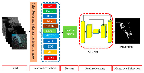
Figure 1.
Segmentation framework of mangrove extraction using deep learning.
2.1. Study Area
The study area is located in the northeast of Hainan Island, including Dongzhaigang National Nature Reserve (DNNR) and its surrounding area of approximately 5 km (Figure 2). DNNR is the first National Nature Reserve for mangroves in China. Dongzhaigang mangrove is the largest coastal beach forest in China, with a total length of 28 km. It is the most well-preserved, most concentrated, continuous, and mature mangrove forest. DNNR is the most resource-rich area of all mangrove types. It is a typical mangrove wetland composed of major mangrove species in southern China and is becoming a major area for mangrove classification research [35]. There are five families and eight genera of mangroves in DNNR. These mangroves contain eleven species, including Bruguiera gymnorhiza Lamk, Bruguiera sexangular Poir, Bruguiera sexangular rhynchopetala, Ceriops tagal, Kandelia candel, Rhizophora stylosa Griff, Sonneratia apetala Buch, Sonneratia cylindria Engler, Aegiceras corniculatum Blanco, Acanthus ilicifolius, and Derris trifoliata. Figure 2 shows that some mangroves are located in intertidal wetlands, such as estuaries, coasts, and islands. Therefore, the integration of water and vegetation characteristics has important guiding significance for the distinction between land vegetation and mangrove vegetation. The MNDWI was closely related to the characteristics of the water body, and it was introduced for extracting the mangroves in this study.
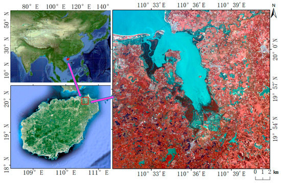
Figure 2.
Location and false color combination of 10 m Sentinel-2 data (Shortwave-infrared reflectance (SWIR), G, and B) of the study area.
2.2. Remote Sensing Data and Preprocessing
The data characteristics of Sentinel-2A MSI (S2) images are shown in Table 1, including basic information, such as wavelength range and spatial resolution of 13 bands. S2 satellite images (Level-1C) were downloaded from the Sentinel Scientific Data Hub (https://scihub.copernicus.eu/dhus/#/home accessed date: 1 March 2020) of the European Space Agency. These images are atmospheric apparent reflectance products after orthophoto correction and subpixel geometric precision correction; thus, the images are not geometrically corrected. The authors used sen2cor to correct the atmosphere of the Level-1C image and obtain the processed bottom-of-atmosphere Level-2A products. The sen2cor atmospheric correlated processor software (version 2.8.0) is a built-in algorithm within software SNAP (Sentinel’s Application Platform) version v6.0. Sentinel-2 data cannot be directly opened with ENVI 5.3.1. To ensure that all the data products had the same pixel size for deep learning for mangrove extraction, we read the Level-C 2A image through SNAP, resampled the band needed by the image to 10 m pixel size, and converted it to a format that could be used by ENVI to facilitate subsequent data processing in ENVI.

Table 1.
The characteristics of Sentinel-2 imagery.
According to previous experiments and previous research results [35,38], the red-edge bands from Sentinel-2 and the SAR data from Sentinel-1 are also useful for differentiating different vegetation types. However, many redundant and even noise data [39] are observed for only mangrove extraction using deep learning after our preliminary research. Therefore, five original bands, namely R, G, B, NIR, and SWIR-1, were selected for the experiments to improve the accuracy of mangrove extraction. In addition, five multispectral indices were obtained by band calculation for mangrove extraction, and their detailed calculation process is shown in Table 2. The PCA1 [11] was computed by the six original bands (including R, G, B, NIR, SWIR-1, and SWIR-2) as the sixth multispectral index. A series of experiments was conducted in Section 3.5, which starts with the five spectral bands. Then, additional data were incorporated to improve the performance of the mechanism in proving the effectiveness of each index.

Table 2.
Calculation method of multispectral indices.
2.3. Deep CNN Structure
The designed architecture is named ME-Net. Inspired by the performance of the fully convolutional networks (FCN) structure in pixel classification, ME-Net is designed with two parts (Figure 3). The first part (top of Figure 3) uses ResNet-101 to extract features, whose kernel is arithmetic mean; the second part (bottom of Figure 3) aims to extract multiscale information and context information in different stages and generate a binary classification map to obtain good mangrove extraction performance.
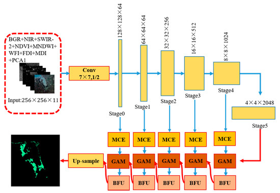
Figure 3.
Architecture of the ME-Net. Arrows represent different operations, among which blue arrows represent convolution and pooling and red represents up-sampling; MCE: multiscale context embedding (MCE); GAM: global attention module; BFU: boundary fitting unit.
In accordance with the size of the feature map, the ResNet-101 network is divided into six stages, namely {Stage 0, Stage 1, …, Stage 5}. We refer to the stage with a larger feature size as the low stage and the stage with a smaller feature size as the high stage. According to our observation, different stages have varying recognition abilities. In the lower stage, the network encodes detailed spatial information. Thus, the low-stage feature map has accurate location information. However, the semantic consistency is poor due to its small receptive field and insufficient spatial context information guidance. At a higher stage, the map has strong semantic consistency because of its large receptive field; however, the location information is relatively inaccurate.
In summary, the lower stage provides more accurate spatial prediction, and the higher stage offers more accurate semantic prediction. On the basis of this observation, we propose a GAM, which guides the lower stage by the context information of the higher stage. In addition, we propose an MCE module and a BFU. The former extracts the multiscale information of mangroves in remote sensing imagery, and the latter combines the boundary of features in the feature map to eliminate some “salt and pepper noise” and “grid artifacts” [40]. These models are introduced in the following sections.
2.3.1. GAM Module
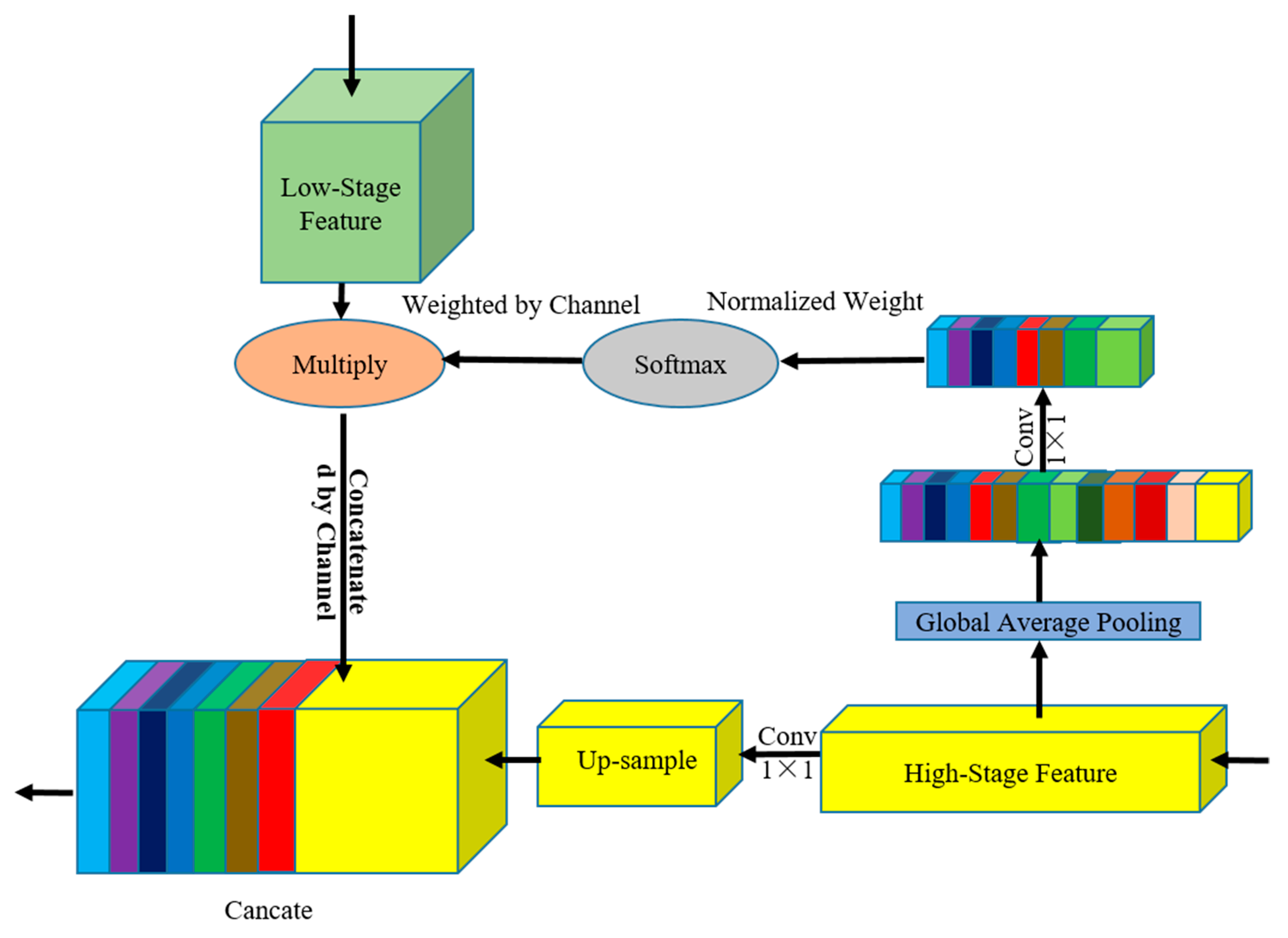
GAM (Figure 4) performs GAP to provide global context information to guide in the low-stage feature map. Global context information provides strong location consistency constraints for feature map in low-stage maps to correct the offset and dislocation of feature location. The structure integrates position consistency guidance information from high-stage feature maps and detailed information from low-stage feature maps. GAM has two branches, namely the global attention information weighting branch and the upsampling branch.
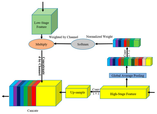
Figure 4.
GAM architecture. Light green squares represent the characteristics of the low-stage maps, and yellow squares represent the high-stage maps. We connected the features of the adjacent stages to calculate the weight vector and then reweighted the low-stage feature map.
Obtaining sufficient information to extract the relationship between channels is difficult because convolution only operates in a local space. To encode the entire spatial feature on a channel as a global feature, GAP is exploited to address the problem, as follows:
where is the value of each feature pixel in channel k, and k ; H is the height; W is the width; and C is the number of channels.
On the weighted branch of the global attention information, we performed GAP on the feature map in the higher stage to generate global context information and conducted a nonlinear 1 × 1 convolution and batch normalization [41]. The nonlinear 1 × 1 convolution is activated by a rectified linear unit (ReLU) or softmax function. The calculation process is shown as follows:
where is the prediction probability of each channel and is the output of each channel.
Finally, the result calculated by softmax is multiplied by each pixel in the low-stage feature map, and the high-stage feature map information is used to guide the low-stage feature map channel to provide context information guidance. The calculation process is shown in Formula (3), as follows:
where is a 3D matrix of H × W × C, W is a column vector of 1 × C, F is the feature map, is the weight of the channel c, and is any pixel value in the feature map of channel c.
In the upsampling branch, the high-stage feature map uses complex encoder blocks, which cost considerable computing resources. In the sampling process from the high-stage feature map to low-stage feature map, 1 × 1 convolution is performed to reduce the channel from the high-stage feature map and integrate the channel information to increase the nonlinear features of decoding layer and reduce the computing load. This module can effectively deal with the feature map of different scales and use a simple method to allow the high-stage feature map to provide consistent constraint information for the low-stage feature map.
2.3.2. MCE Module
Inspired by the inception architecture in GoogleNet [42,43,44] and atrous spatial pyramid pooling (ASPP) module in DeepLab [23], we propose an MCE module (Figure 5). This module extracts multiscale context information by four convolution kernels of different sizes and compresses the number of channels to reduce the computational load.
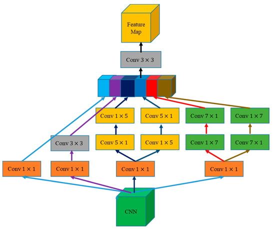
Figure 5.
MCE architecture. The green box is the input feature map, the yellow box is the output feature map, the rectangle is the convolution operation of different sizes of convolution kernel, and the colored box is the multiscale feature map in series according to the channel.
The designed MCE combines the feature maps of context information with the global information of the high-stage feature map in the GAM. We used 1 × 1, 3 × 3, 5 × 5, and 7 × 7 convolution in MCE to effectively extract context information from feature maps at different stages, where 1 × 1 convolution is used to reduce the dimension of the feature map. The 1 × k + k × 1 and k × 1 + 1 × k convolutions were combined in MCE instead of k × k to avoid a large convolution kernel or global convolution. After splicing the multiscale information in accordance with the channel, 3 × 3 convolution was used to roughly integrate the multiscale information and adjust the number of channels.
2.3.3. BFU Module
Inspired by the mask regions with CNN (R-CNN [45]), BFU (Figure 6) is designed to correct the boundary position of the features by two continuous 3 × 3 convolution kernels. On the one hand, the BFU eliminates the “grid artifacts” caused by the context embedding of the feature maps in different stages. On the other hand, BFU solves the aliasing effect caused by the convolution and pooling operations. In addition, a skipped connection is added to supervise the semantic of the feature map after boundary modification. This approach speeds up the flow of information in the network and optimizes the performance of boundary fitting.

Figure 6.
BFU architecture. The green box is the feature map, the yellow rectangle is the convolution operation, the brown rectangle is the batch normalization(BN) operation, the orange ellipse is ReLU, “+” represents that a feature map with the same size is added in accordance with the pixel position, the blue arrow represents the skipped connection, and the red box represents the feature mapping.
The proposed BFU can be understood as a 1 × 1 convolution and a residual module. In the BFU, 1 × 1 convolution is used to learn the information of different channels while reducing the number of channels of the original feature map to reduce the computation amount. The residual module is used to smoothen the feature map and eliminate “grid artifacts” and aliasing effects.
2.4. Loss Function Optimization
Mangrove extraction is a binary classification problem; thus, binary cross-entropy loss and Dice loss function value at each pixel are used, as follows:
where represents the set of pixel ground truth labels, and denotes the set of pixel prediction results.
The strategy of deep supervision was applied in the training of the ME-Net model. A supervision function was added to the hidden layer to reduce the effects of the gradient disappearance and improve the speed of model convergence. As shown in Figure 7, we upsampled the output of the third stage feature map of the ME-Net to resize it to its original image size. A binary cross-entropy loss function Loss2 was added as the supervision of the middle hidden layer to optimize the learning process. Loss1 was used to optimize the overall network. We also increased the weight to balance the two loss functions.
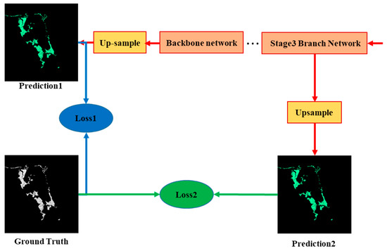
Figure 7.
Two loss functions in ME-Net.
3. Results and Discussion
3.1. Preprocessing of Experimental Data
In combination with field sampling and visual interpretation of Google Earth satellite images, we manually marked the original remote sensing imagery by ArcGIS 10.2 to obtain the ground truth labels. These training samples were labeled under the supervision of several experts, who are professionals in mapping mangrove extent and species, to ensure that these marked samples are correct. We resampled all the bands to the same size to perform band calculations by ENVI 5.3 software to calculate the multispectral indices. The spatial resolution of Sentinel-2 remote sensing imagery used in the experiments is 10 m. This work labeled the remote sensing images by consensus of several experts to ensure correct classification of mangroves. We selected the sentinel-2A remote sensing data acquired on 13 April 2018, in Hainan Dongzhaigang National Nature Reserve in China. The data comprised 2093 2214 pixels after preprocessing, such as cropping. The remote sensing imagery was clipped by a 256 256 sliding window with a 32-pixel step. We used random left and right flips and up and down flips and increased “salt and pepper noise” for some datasets to increase the size of the datasets and avoid filling null values. Furthermore, we randomly rotated the clipped samples by 90°, 180°, and 270° and randomly scaled the sample data in five scales. The dataset had 5120 original images with 256 256, where 20% (1024 images) were used as test sets for validating the proposed model, and 80% (4096 images) together with 1280 augmented images were utilized as the training sets for training the proposed model. During the training, 85% of the training sets were used to train the ME-Net model, and 15% of the training sets were utilized to validate the ME-Net model.
3.2. Implementation Details
3.2.1. Input Data
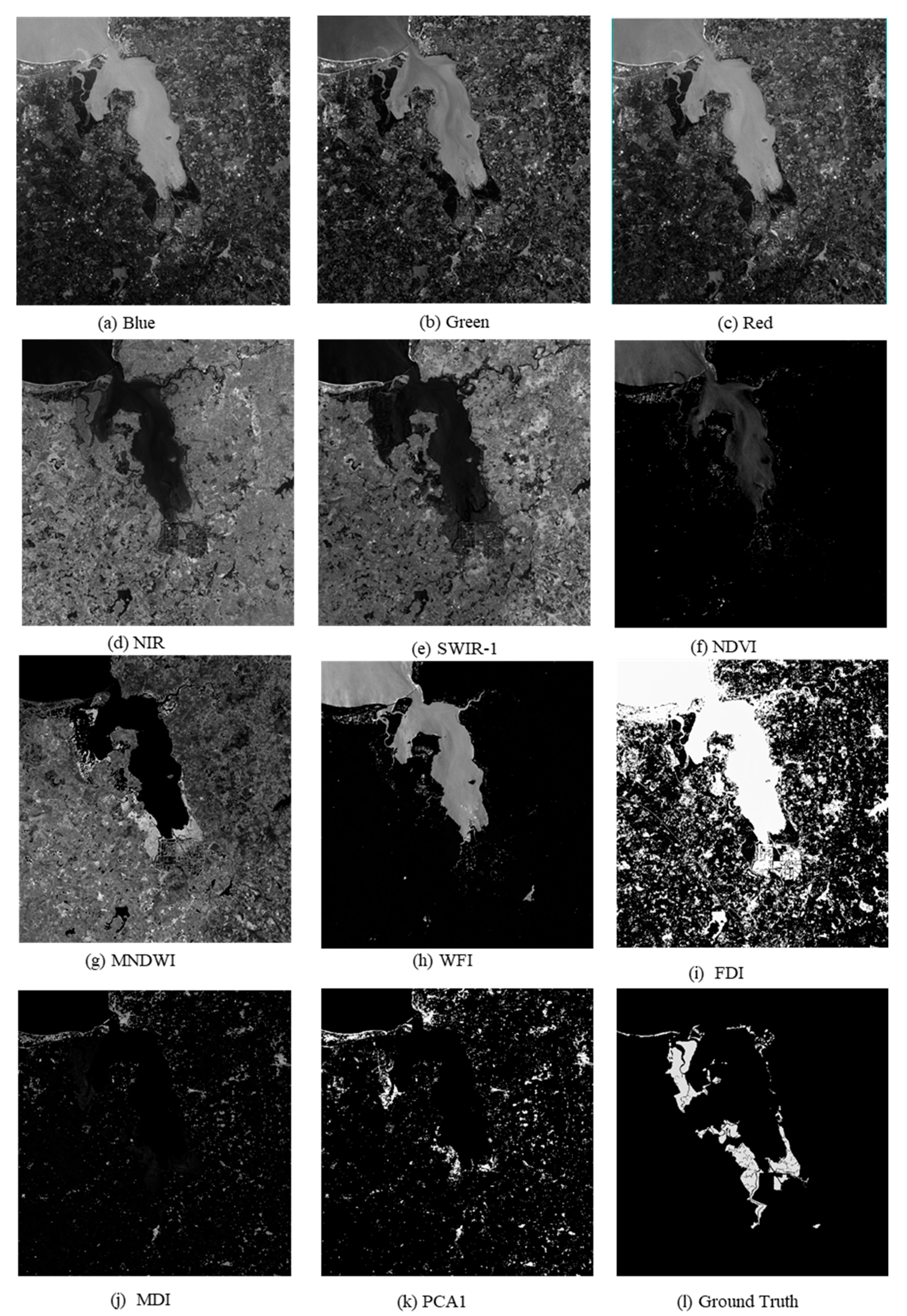
All the prepared sample data, including five original bands, namely, R, G, B, NIR, and SWIR-1; six multispectral indices, namely NDVI, MNDWI, FDI, WFI, MDI, and PCA1; and the corresponding ground truth labels were used as inputs to the ME-Net model. The input data used by the deep neural network are shown in Figure 8.
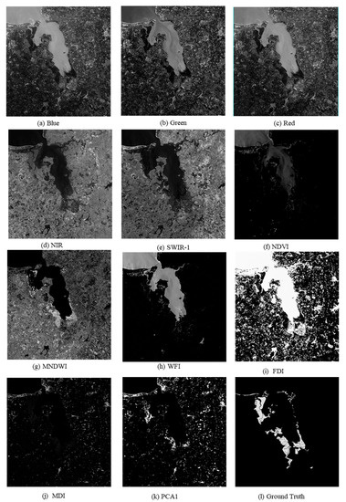
Figure 8.
Samples of the Sentinel-2 remote sensing imagery used in the experiments.
3.2.2. Set of Hyperparameters
During the training of the ME-Net model, transfer learning was used to improve the generalization ability of the model. The ME-Net was designed on the basis of Res-Net, which was trained before it was inserted into the whole model. Moreover, minibatch stochastic gradient descent (SGD) [29] was used to minimize the loss function and update the weight parameters in backpropagation. In the experiment, the batch size was 8, the momentum was 0.9, and the weight decay was 0.0001. The SGD optimization function is greatly affected by the initial learning rate. Thus, the learning rate of the ME-Net model was set to 0.01 to obtain better performance and speed up the processing. We used the “poly” learning rate strategy, in which the initial rate was multiplied by . The number of training epochs was 100, the number of iterations in each epoch was 200, and 32 samples were used in each iteration.
3.3. Experimental Results
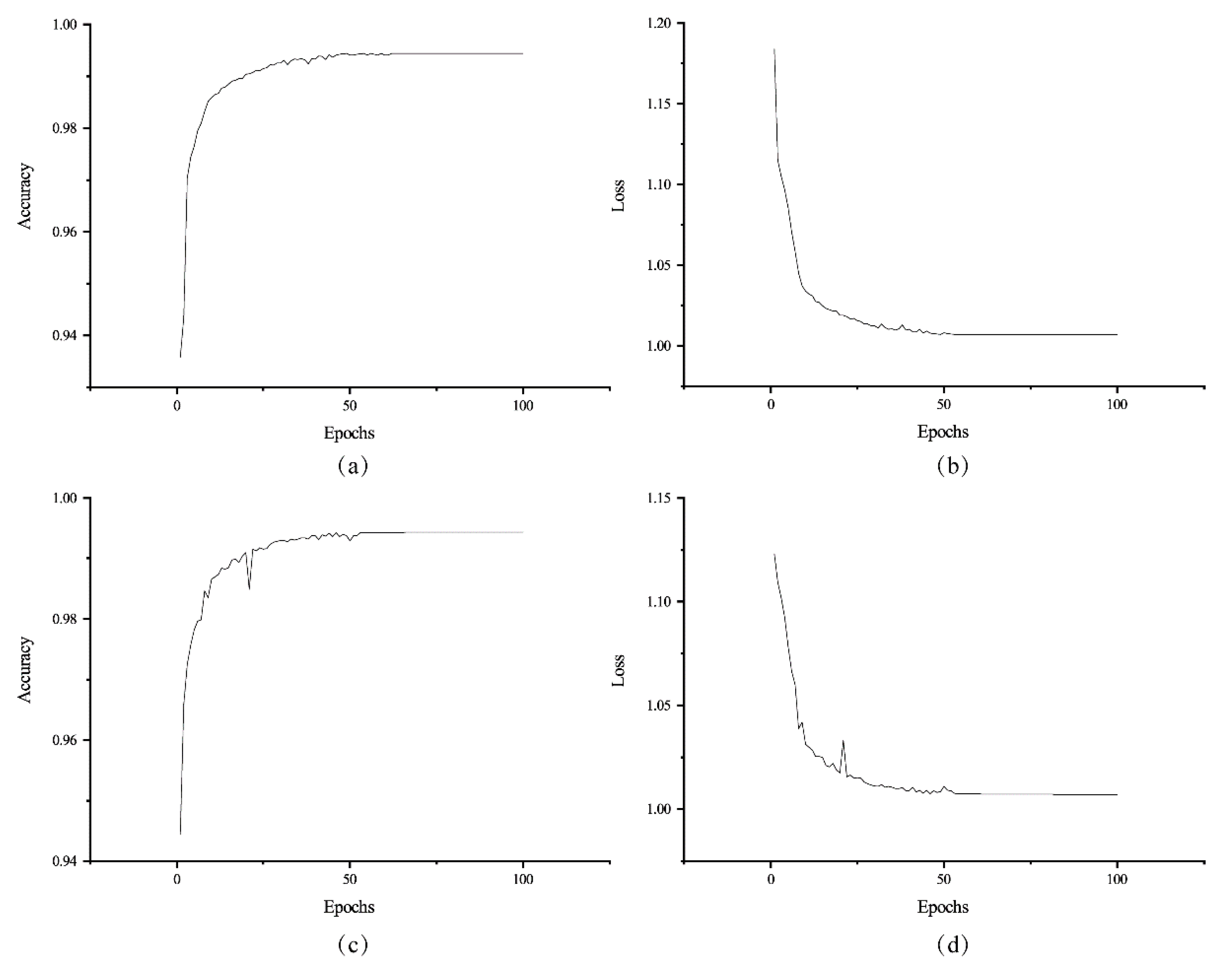
The proposed ME-Net model was implemented using the open-source Tensorflow and Keras framework provided by Google in Python. The code of the pixel classification model was executed on Windows 10 platform with four NVIDIA GTX 1080Ti GPUs (12 GB RAM per GPU). After 100 epochs, the ME-Net model achieved state-of-the-art results on the datasets (Figure 9).

Figure 9.
Accuracy and loss of ME-Net for training the datasets. The training accuracy (a) and loss (b) change with the epochs on the training datasets. The validating accuracy (c) and loss (d) change with the epochs on the validating datasets.
We used pixel Intersection over Union (IoU) as the accuracy measure to quantitatively evaluate the performance of the ME-Net model in extracting mangroves from remote sensing images. IoU is defined as:
where represents the set of pixel ground truth labels; represents the set of pixel prediction results; “∩” and “∪” represent the calculation operation of intersection and union, respectively; and | • | represents the number of pixels in the calculation set.
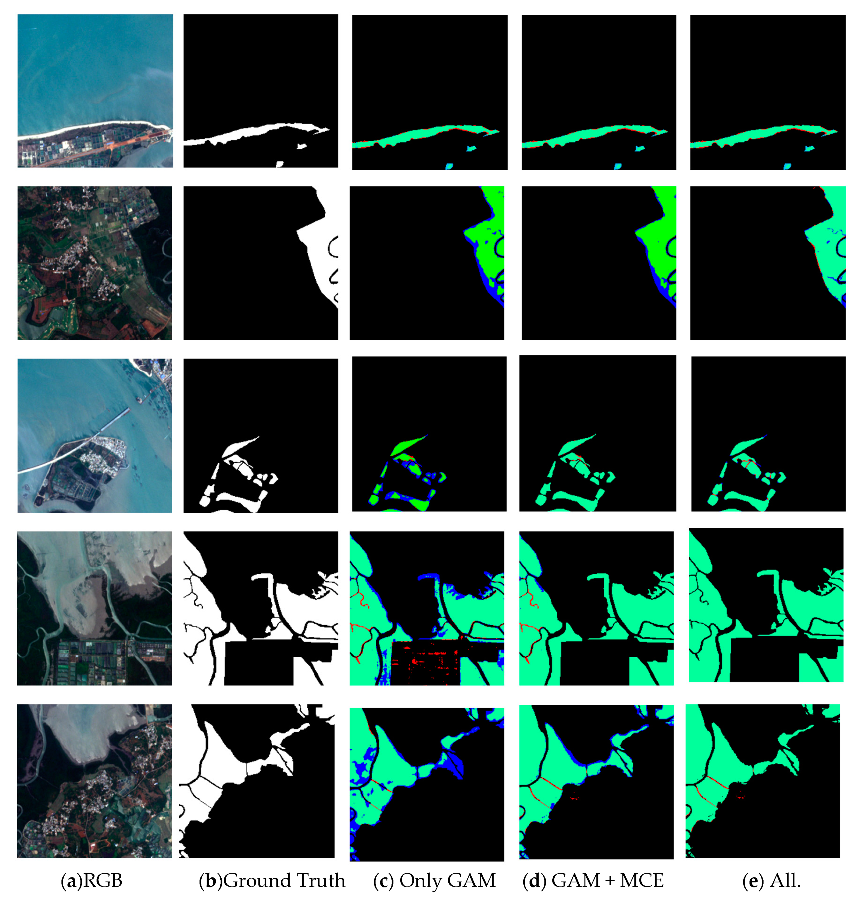
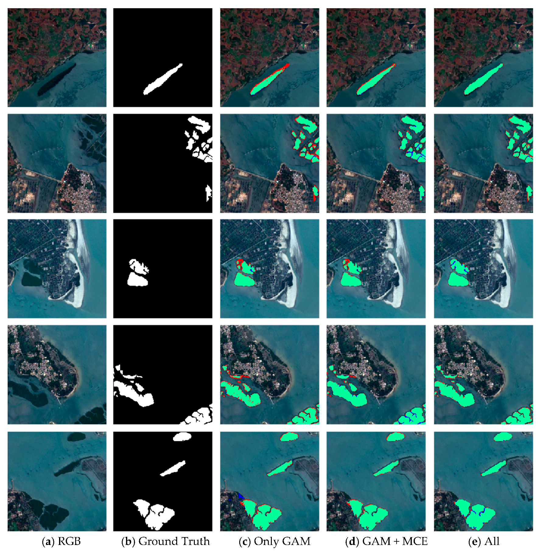
The overall accuracy of the trained ME-Net reached 97.49%, and the F1 score reached 96.56% (Table 3), which proved that the proposed model was excellent in extracting mangroves from remote sensing imagery. To prove that the method is universal, we used some data from roadside areas, estuaries, bays, shoals, and islands to verify the method. In the ablation study, we successively added GAM, MCE, and BFU to explore the impact of each module on the experimental results (Figure 10).

Table 3.
The metrics of our best model, including precision, recall, F1 score and IoU value for mangrove extraction from remote sensing imagery.
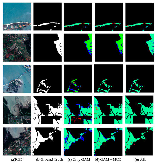
Figure 10.
Results of mangrove extraction in different environments by different modules in ME-Net. The original images (a), the corresponding ground truth (b) and predictions (c–e) are presented. Green, red, blue, and black represent true positive (TP), false positive (FP), false negative (FN), and true negative (TN) respectively.
In various experimental scenarios, we compared the results (Figure 10) to explore the impact of different modules in the ME-Net model on the performance of mangrove extraction. Although most mangroves in the remote sensing imagery can be accurately extracted by using the GAM, the blue area is greatly reduced after the MCE is added. The multiscale information is beneficial to improve the accuracy of mangrove extraction. However, the prediction results of the fourth row of mangroves show that many problems, such as “salt and pepper noise”, blurred boundaries, and misclassified or missed pixels, still exist. To solve these problems, BFU was introduced into the model. In addition, the red and blue areas were reduced at different scales. This finding fully showed that the BFU made further constraints on the pixel classification information of mangroves, and the predicted results were further optimized.
3.4. Evaluating the Model by a New Dataset
The overall accuracy and F1 score reached over 96.56% in the dataset of DNNR. We have made a new dataset to prove that the designed model has the generality to extract mangroves from remote sensing imagery. This dataset is based on the study area of He’anpian Mangrove Nature Reserve in Southeast Zhanjiang City, Guangdong Province. The geographical coordinates of the study area are 110°17′49″–110°27′40″ E and 20°34′11″–20°43′48″ N. The mangroves labeled by experts in the remote sensing images were treated as the ground truth. The precision of the trained ME-Net for the new dataset reached 96.00%, and the F1 score reached 95.55% (Table 4).

Table 4.
The performance for the trained model on a new dataset.
A series of experiments was implemented to qualitatively prove that our model has the generality for a new dataset (Figure 11). When trained models were applied to the new dataset, the red and blue areas were greatly reduced by using the GAM, MCE, and BFU. The experimental results of mangrove extraction by different modules in ME-Net showed that the proposed method can effectively extract mangroves, and it has good generalization ability.

Figure 11.
Results of mangrove extraction in a new mangroves region by different modules in ME-Net. The original images (a), the corresponding ground truth (b), and predictions (c–e) are presented. Green, red, blue, and black represent true positive (TP), false positive (FP), false negative (FN), and true negative (TN) respectively.
3.5. Effects of Sample Data on the Results
The Sentinel-2 remote sensing imagery can extract the mangrove area on the ground through the false-color image composed of SWIR, G, and B bands. However, the phenomena of “same object with different spectra” and “different objects with the same spectra” are observed because of the different living environments and distributions of mangroves. Accordingly, the mangroves in some areas are missing or misclassified. We need to fully use the multiband information of remote sensing information and mine the multispectral indices to improve the accuracy of mangrove classification, which is beneficial to the extraction of mangroves. In this research, five original bands were selected from the sample data, namely, B, G, R, NIR, and SWIR-1. In addition, six multispectral indices (NDVI, MNDWI, FDI, WFI, MDI, and PCA1) were computed to mine the spectral, textural, and shape information between mangrove and non-mangrove features. We used the pretrained ResNet-101 weight on the ImageNet datasets as the initial weight of our basic feature extraction network and upsampled the output in accordance with the structure of the FCN referred to as ResNet-based FCN. Under the ResNet-based FCN structure, we obtained the actual color images of the B, G, and R bands as the initial input data of the experiment and constantly added new input data to the experiment (Table 5). Adding some original band information and multispectral indices can effectively improve the results of mangrove prediction. The performance of network classification increased from 86.64% to 92.13%.

Table 5.
Effect of original band and multispectral index to the classification result of mangrove under the ResNet-based FCN structure.
Table 5 shows that the IoU increased by 0.69% with the addition of NIR and SWIR-1. After adding the six multispectral indices, IoU increased by 4.80%. Moreover, the effects of NDVI, MNDWI, and MDI had a remarkable effect on the results. The controlling variable method was used to analyze the effect of each multispectral index for exploring the performance impact of these multispectral indices on the mangrove extraction results (Table 6).

Table 6.
Effect of normalization difference vegetation index (NDVI), modified normalized difference water index (MNDWI), and mangrove discrimination index (MDI) on the result of mangrove extraction under the ResNet-based FCN.
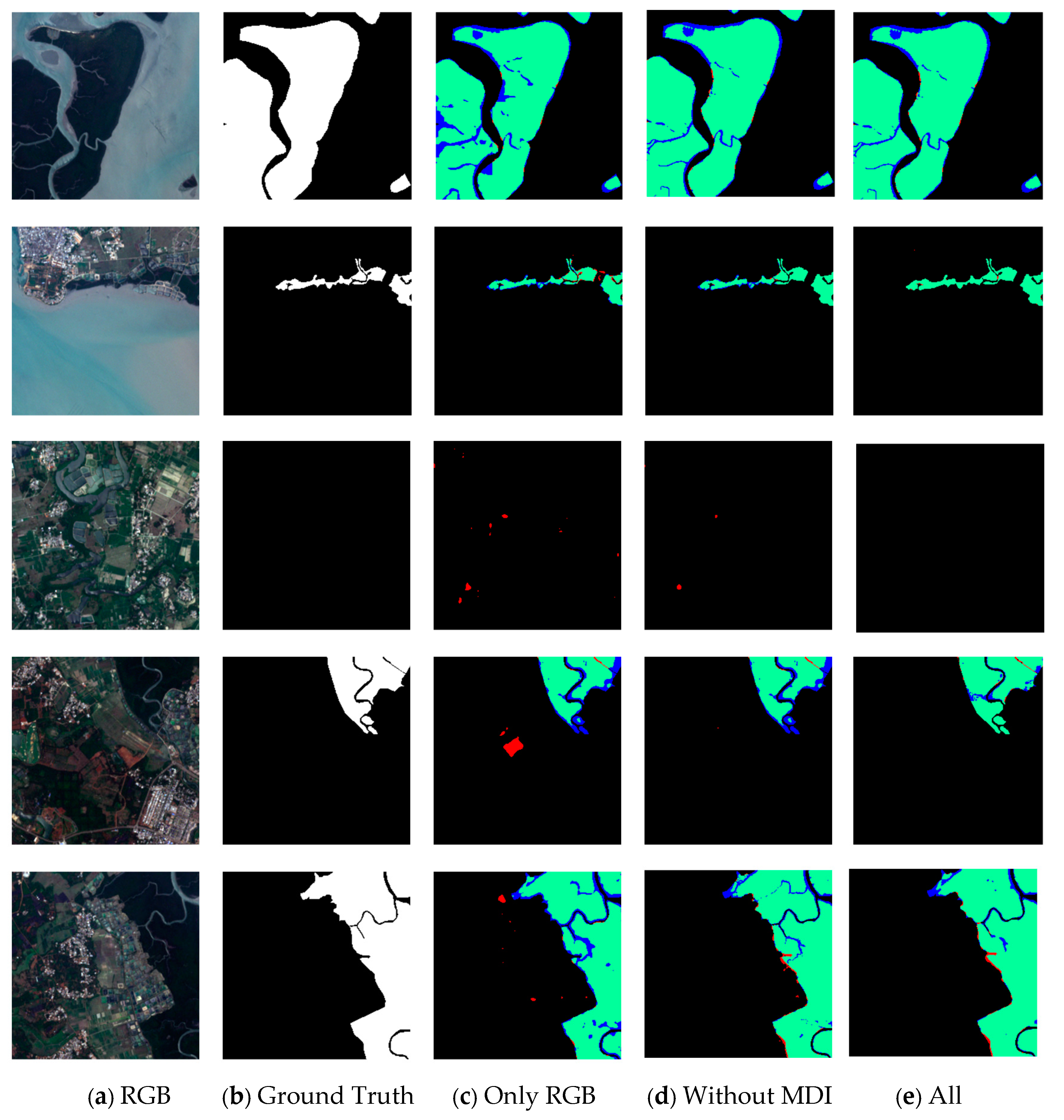
Table 6 shows that when NDVI, MNDWI, and MDI were excluded, their IoU indicators were reduced by 0.81%, 1.2%, and 1.37%, respectively. When only the RGB bands were used as inputs, IoU was reduced by 5.49%. The experimental data showed that the MNDWI and MDI can significantly improve the performance of mangrove extraction. The MNDWI was closely related to the characteristics of the water body, and mangroves were located in intertidal wetlands, such as estuaries, coasts, and islands, which coincides with the difference between Figure 12e,c. Therefore, the integration of water and vegetation characteristics has important guiding significance for the distinction between land vegetation and mangrove vegetation. In addition, the comparative analysis of the spectral characteristics showed that the spectral reflectance of mangroves in SWIR-2 is lower than that of terrestrial vegetation, which also confirmed the potential reason why MDI could significantly improve the classification results. Figure 12 shows that in remote sensing imagery, some land vegetation distributed near shallow land surface areas, such as lakes and wetlands, can be further distinguished from mangroves by MDI.
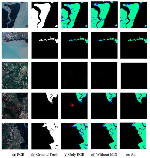
Figure 12.
Effect of some sample data on the result of mangrove exaction under the ME-Net model. The first column (a) shows the actual color of the remote sensing imagery; the second column (b) shows the corresponding ground truth; the third column (c) shows the prediction result of the model after adding only three bands of RGB; the fourth column (d) shows the prediction result after adding MDI; the fifth column (e) shows the prediction result after adding five original bands and six multispectral indices. Green, red, blue, and black represent the TP, FP, FN, and TN, respectively.
In different experimental scenarios, we compared the results (Figure 12) to explore the impact of adding different sample data to the ME-Net model on the performance of mangrove extraction (the IoUs for data are shown in Table 7). The experiment results showed that some FP pixels would appear in the prediction results of the model when only three bands, R, G, and B, were used. The actual color of the remote sensing imagery indicated that it is a classical phenomenon of “different objects with the same spectra”. Most features represented by these FP pixels were wetlands on the land surface or dense woodland growing in shallow water areas, with similar spectral characteristics in mangrove areas, thereby resulting in a large number of categorical misjudgments. The experimental results showed that red and blue regions decrease in varying degrees, characterized by a more significant reduction in the red areas. The results showed that rich multiband data and multispectral indices were conducive to a more detailed pixel-level classification of mangroves. The prediction results with and without the MDI index are shown in the fourth and fifth columns of Figure 12, respectively. The comparative results of these columns clearly show that the classification of marginal areas was greatly improved after the MDI index was added, such as the river and forest edge of the mangrove area. This finding indicated that the MDI index contains the structural and textural information required for mangrove classification.

Table 7.
The IoU for data in Figure 12 from rows 1 to 5.
3.6. Influence of Network Structure and Training Skills
In the pixel classification of remote sensing imagery, we need to simultaneously complete the classification and location of mangroves. However, the classification and location in the deep learning algorithm are contradictory. The high-stage feature map of CNN is excellent at solving the classification problem. However, reconstructing the prediction result of binarization of the original resolution is difficult because convolution and downsampling lose a large amount of location information. Therefore, we proposed GAM and used the classification information learned by the high-stage feature map as a weight to guide the location reconstruction of the low-stage feature map. Prior to the reconstruction of location information by GAM, MCE was used to extract features from the low-stage feature maps, and the multiscale information was fused. Subsequently, BFU was used to eliminate problems, such as aliasing and “grid artifacts” in the convolution process and pooling operation and “salt and pepper noise” in image classification. We used the controlling variable method to analyze the influences of each element to explore the effects of GAM, MCE, and BFU on the mangrove extraction results (Table 8).

Table 8.
Effects of GAM, MCE and BFU on the extraction results of mangroves.
In Table 8, DS represents deep supervision. DA represents data augmentation method, including adding noise and left and right flip and rotation deformation. C1 and C3 represent the size of the convolution kernel on the decoding branch of GAM. GAP and GMP represent GAP and global max pooling, respectively. C1355 indicates that the sizes of the convolution kernel of the four branches of MCE are 1 × 1, 1 × 1 + 3 × 3, 1 × 1 + 1 × 5 + 5 × 1, and 1 × 1 + 5 × 1 + 1 × 5. C1357 indicates that the sizes of the convolution kernel of the four branches of MCE are 1 × 1, 1 × 1 + 3 × 3, 1 × 1 + 5 × 5, and 1 × 1 + 7 × 1 + 1 × 7.
The experimental data in Table 8 showed that GAM can effectively extract global contextual attention information and significantly improve the performance of mangrove extraction from 92.13% to 95.55% compared with ResNet-based FCN. Different global pooling methods lead to varying results. GAP improved the performance of the model by 0.17% compared with GMP. Therefore, GAP was used in the final model. Moreover, the performance of ME-Net improved by adding the MCE module, and the IoU of mangrove classification increased from 95.71% to 96.16%. The results of C1355 and C1357 showed that different sizes of convolution kernels can extract diverse scale information, and the information of various scales improved the classification of mangroves. When we used BFU instead of MCE in the experiment, IoU increased from 95.71% to 95.89%. On the basis of MCE, IoU increased by 0.73% when BFU is added to the network. This finding showed that BFU is beneficial to mangrove classification, and that the combination of MCE can enable GAM to obtain more accurate and rich global mangrove information. We conducted a series of comparative experiments to more intuitively show the effect of BFU on the mangrove classification results. The results (Figure 10) clearly showed that the BFU module can simultaneously improve the boundary of pixel classification and eliminate some noise. Two training skills were also used to improve network performance, namely data augmentation, and deep supervision. Some comparative experiments were conducted to explore the influence of these training skills on the results of pixel classification. The results (the last three rows in Table 8) showed that both approaches improve the model performance.
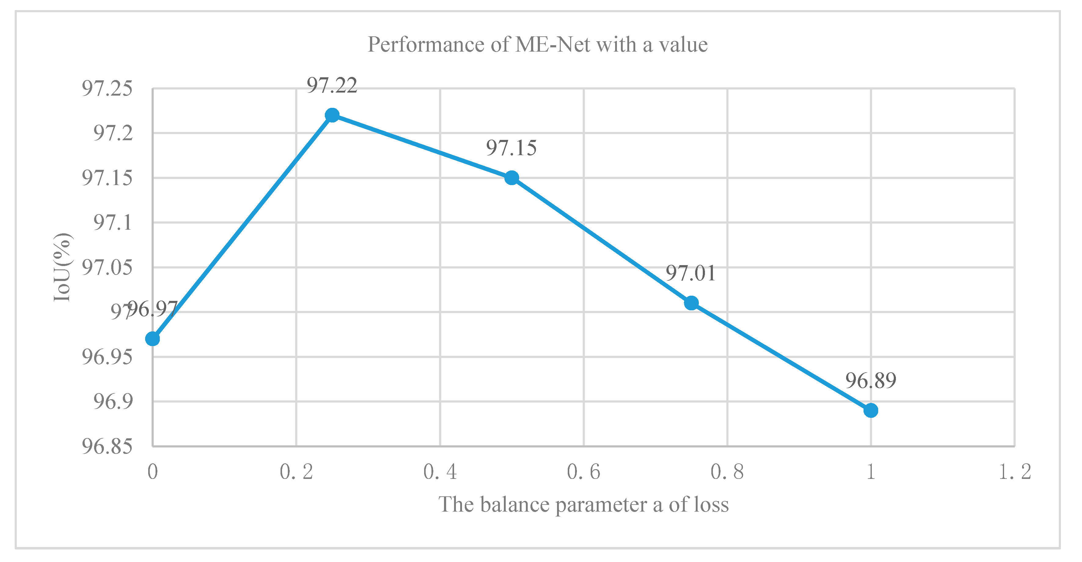
We added a final loss function at the end of the main branch of ME-Net and a second loss function at the end of the ResNet-101 network to solve the difficult problems of the deep neural network optimization. The first loss function optimized the pixel classification performance of the entire network. Meanwhile, the second function optimized the feature extraction process of ResNet-101. We added a balance weight a to the second loss function. We used five different values of 0, 0.25, 0.5, 0.75, and 1 to approximately determine the value of a and further analyze the effect of deep supervision on the network performance improvement. In Figure 13, under the same conditions, the effect of the optimization model was the best, and the accuracy was 97.22% when the balance weight was equal to 0.25. Finally, the experiment using various methods and techniques indicated that the performance of the ME-Net model was improved to 97.48%.
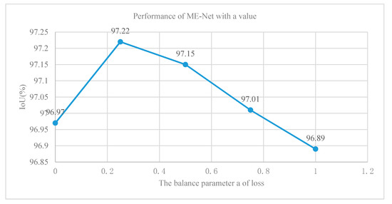
Figure 13.
Results of ME-Net with different values of balance weight a.
3.7. Model Analysis
This work was compared with some new methods, including FCN [31], SegNet [30], DilatedNet [46], U-Net [21], PSPNet [22], DeepLab series [23,24,47], and Mask R-CNN [48], to evaluate the effectiveness of the proposed ME-Net model in mangrove extraction from remote sensing imagery. All methods were trained, validated, and tested on the same datasets for an objective and impartial finding. The comparative test results are shown in Table 9.

Table 9.
Experimental results of ME-Net and other methods.
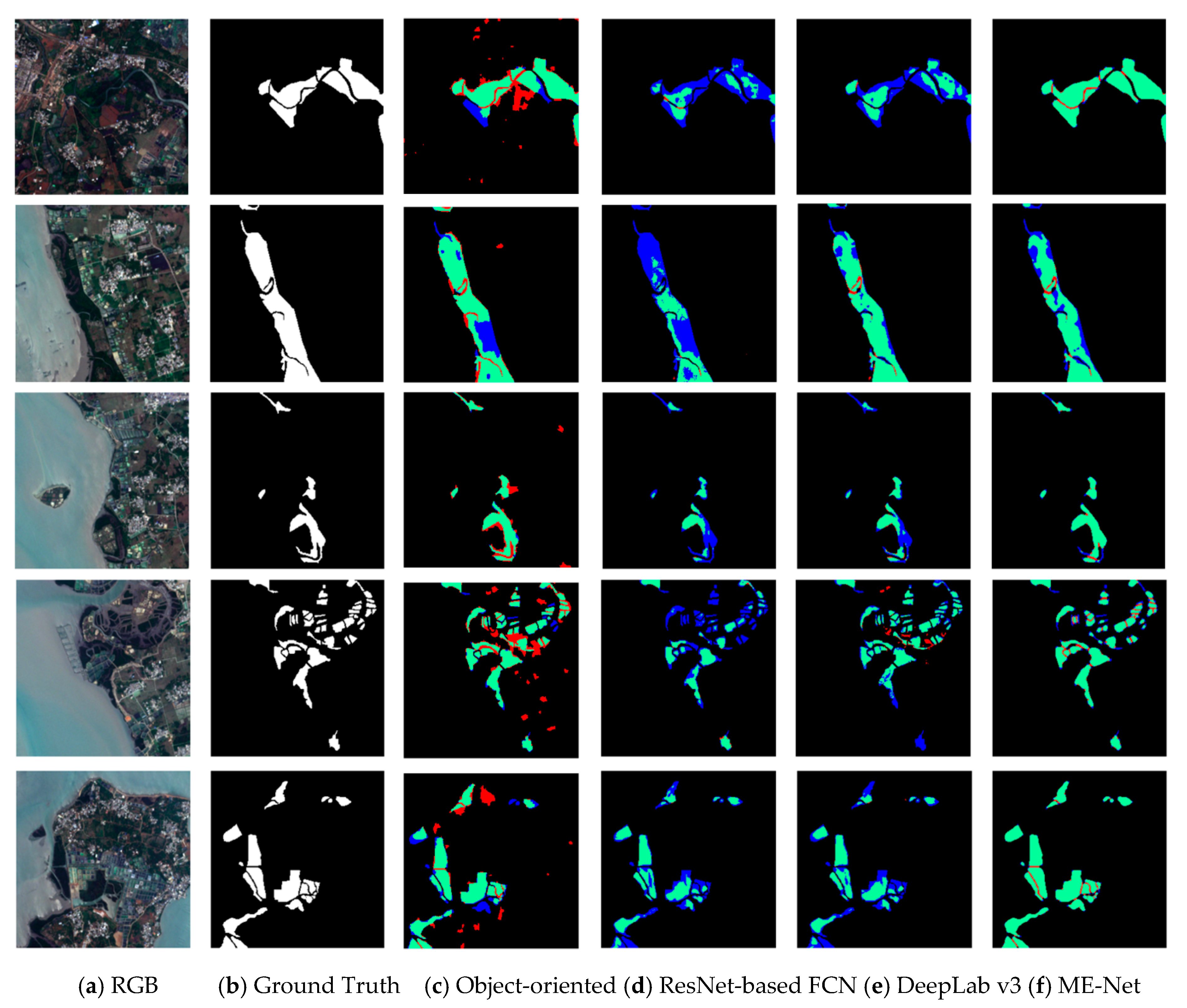
Table 9 indicates that our proposed ME-Net model effectively performed in the mangrove extraction tasks. We have achieved the highest IoU (96.97%) without using the methods of data augmentation and deep supervision. We selected samples to more intuitively show the impact of different methods on mangrove extraction performance, the classification results of which are difficult to predict. In addition, the prediction results of ResNet-based FCN, DeepLab v3, and ME-Net model were compared (Figure 14).
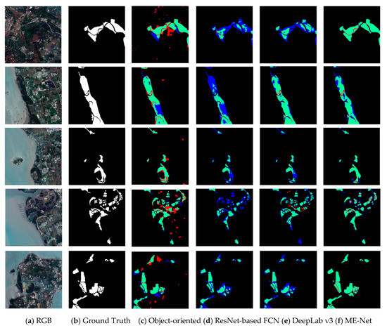
Figure 14.
Performance of different pixel classification models in mangrove extraction. The first column (a) shows the actual color of the remote sensing imagery; the second column (b) shows the corresponding ground reality; the third column (c) shows the prediction result of object-oriented by ENVI; the fourth column (d) shows the prediction result of ResNet-based FCN model; the fifth column (e) shows the prediction result of DeepLab v3 model; the sixth column (f) shows the prediction result of the ME-Net model. Green, red, blue, and black represent the TP, FP, FN, and TN, respectively.
Some scenes, which were difficult to classify, such as nonblock, sporadic scattered, and coastal strip edges, were used in the experiments to increase the contrast of the classification results. The object-oriented model failed to extract mangrove compared with the deep learning methods (Figure 14 and Table 10). The classification results of different methods were compared in detail. The result showed that the blue area in the prediction results of the ResNet-based FCN model was significantly more than that of the other methods. The existence of a large number of FP pixels showed that some pixels that should belong to mangroves were been detected by the model, and the model has an under-fitting problem. The under-fitting of the model indicated that a large amount of classification information was not learned by the model. The data in the third and fourth columns in Figure 14 indicate that the blue area in the prediction result of DeepLab v3 was much less than the other areas (the IoU for data are shown in Table 10). This finding indicated that the data fitting ability of the DeepLab v3 model was stronger than that of the ResNet-based FCN. The analysis of the network structure of DeepLab v3 model showed that the model using dilated convolution and ASPP can effectively capture multiscale information and improve the performance of mangrove extraction. Finally, we found that the blue region was greatly reduced compared with the proposed ME-Net model; however, the red region was partially increased. This finding shows that the ME-Net model has strong data fitting ability and can be effective for pixel classification. However, part of the boundary was over-fitted and overcompensated to the prediction results due to the role of the BFU, and some pixels that belong to nonmangroves were misjudged as mangroves. Although some over-fitting cases were found, the overall performance of ME-Net model in mangrove extraction was still much better than that of the other pixel classification models. In addition, the noise in the remote sensing imagery will decrease the accuracy of ME-Net, and the denoising method will be exploited to address this problem in the future [48,49].

Table 10.
The IoU for data in Figure 14 from rows 1 to 5.
4. Conclusions
Accurate extraction of mangroves from remote sensing imagery is important to dynamically map and monitor the distribution area of mangroves. However, mangroves have different geometric appearances and spectral and textural features. Accordingly, accurate extraction of mangroves faces great challenges. Datasets for mangrove extraction are developed, and a new pixel classification framework, ME-Net, is proposed. The ME-Net is trained and tested to explore the impact of different sample data and feature learning modules on the extraction of mangrove results. In this research, the controlling variable method is used to experiment on each band and multispectral index. The results show that the selection of multiband data and the multispectral indices are beneficial to the extraction of mangroves. In the network model, GAM is proposed to provide global context information to guide in the low-stage feature map, and an MCE module is proposed to extract multiscale information. BFU is applied to optimize the classification results. In the data preprocessing, multiband remote sensing imagery and manually created multispectral indices are used to improve the performance of mangrove pixel classification. The results of the experiments on multiple remote sensing imagery indicate that the ME-Net model can effectively integrate a large number of sample data, which can effectively solve the problem of data redundancy and mine abstract semantic information and location information in remote sensing imagery. The proposed approach can successfully extract mangroves in each scene. The results show that the framework is effective and feasible in improving the classification performance of mangroves in different coastal areas.
This work aims to show the success of the proposed GAM, MCE, and BFU approaches to the mangrove extraction issue. We demonstrated the capability of our new deep learning model for mangrove extraction. This study focuses on our new deep learning model (ME-Net). We successfully demonstrated that deep learning methods can be exploited to extract mangroves. We conducted many groups of experiments to demonstrate that our new deep convolutional neural network for extracting mangrove (ME-Net) has the capability to automatically extract mangrove, and it performs better than other typical deep learning methods.
An effective method is provided to improve the classification performance of remote sensing imagery. However, the model still has some unsolved problems. Future work will focus on the following aspects: an end-to-end pixel classification model should be implemented through residual module and convolution to achieve better results in boundary-fitting tasks instead of dense-CRF to a certain extent and develop a simple training process of the model. However, this model exhibits some shortcomings compared with dense-CRF; that is, it cannot effectively combine input data similar to dense-CRF to obtain pixels with similar colors and adjacent positions for a more consistent classification. Additionally, the spatial computational intensity grid [50] is exploited to improve the parallel performance of ME-Net in the next work.
Geophysical setting has an extremely important influence on the distribution of mangrove areas, especially some naturally growing mangrove areas. The mangrove wetland is located in the intertidal zone and is closely related to the characteristics of the water body. Hence, we will consider using remote sensing imagery of different time series to extract natural mangrove regions in future research. Moreover, the intelligent system indicated that the right bands and indices are important for mapping mangroves. Next, we will research how to use the knowledge graph methods to find the right bands and indices.
Author Contributions
M.G. and Y.X. proposed the network architecture design and the framework of extracting mangrove. M.G., C.L., and Z.Y. performed the experiments and analyzed the data. Y.X. and Z.Y. wrote the paper. Y.H. revised the paper and provided valuable advice for the experiments. All authors have read and agreed to the published version of the manuscript.
Funding
This study was financially supported by the National Natural Science Foundation of China (Nos. 41971356, 41701446, 42001340) and the Open Fund of Key Laboratory of Urban Land Resources Monitoring and Simulation, Ministry of Natural Resources (KF-2020-05-011).
Institutional Review Board Statement
Not applicable.
Informed Consent Statement
Not applicable.
Data Availability Statement
Not applicable.
Acknowledgments
The authors thank Dezhi Wang for helping guiding the research.
Conflicts of Interest
We declare that we have no conflict of interest.
References
- Giri, C.; Ochieng, E.; Tieszen, L.L.; Zhu, Z.; Singh, A.; Loveland, T.; Masek, J.; Duke, N. Status and distribution of mangrove forests of the world using earth observation satellite data. Glob. Ecol. Biogeogr. 2011, 20, 154–159. [Google Scholar] [CrossRef]
- Liao, B.W.; Zhang, Q.M. Area, distribution and species composition of mangroves in China. Wetl. Sci. 2014, 12, 435–440. [Google Scholar]
- Giri, C. Observation and Monitoring of Mangrove Forests Using Remote Sensing: Opportunities and Challenges. Remote Sens. 2016, 8, 783. [Google Scholar] [CrossRef]
- Held, A.; Ticehurst, C.; Lymburner, L.; Williams, N. High resolution mapping of tropical mangrove ecosystems using hyperspectral and radar remote sensing. Int. J. Remote Sens. 2003, 24, 2739–2759. [Google Scholar] [CrossRef]
- Kanniah, K.D.; Sheikhi, A.; Cracknell, A.P.; Goh, H.C.; Tan, K.P.; Ho, C.S.; Rasli, F.N. Satellite images for monitoring mangrove cover changes in a fast growing economic region in southern Peninsular Malaysia. Remote Sens. 2015, 7, 14360–14385. [Google Scholar] [CrossRef]
- Kirui, K.B.; Kairo, J.G.; Bosire, J.; Rudra, S.; Briers, R.A. Mapping of mangrove forest land cover change along the Kenya coastline using Landsat imagery. Ocean Coast. Manag. 2013, 83, 19–24. [Google Scholar] [CrossRef]
- Thakur, S.; Mondar, I.; Ghosh, P.B.; Das, P.; De, T.K. A review of the application of multispectral remote sensing in the study of mangrove ecosystems with special emphasis on image processing techniques. Spat. Inf. Res. 2020, 28, 39–51. [Google Scholar] [CrossRef]
- Giri, C.; Pengra, B.; Long, J.; Loveland, T.R. Next generation of global land cover characterization, mapping, and monitoring. Int. J. Appl. Earth Obs. Geoinf. 2013, 25, 30–37. [Google Scholar] [CrossRef]
- Tian, S.; Zhang, X.; Tian, J.; Sun, Q. Random Forest Classification of Wetland Landcovers from Multi-Sensor Data in the Arid Region of Xinjiang, China. Remote Sens. 2016, 8, 136–141. [Google Scholar] [CrossRef]
- Yu, Q.; Gong, P.; Clinton, N.; Biging, G.; Kelly, M.; Schirokauer, D. Object-based Detailed Vegetation Classification with Airborne High Spatial Resolution Remote Sensing Imagery. Photogramm. Eng. Remote Sens. 2006, 72, 799–811. [Google Scholar] [CrossRef]
- Xu, Y.; Wu, L.; Xie, Z.; Chen, Z. Building extraction in very high resolution remote sensing imagery using deep learning and guided filters. Remote Sens. 2018, 10, 144. [Google Scholar] [CrossRef]
- Wang, C.; Chen, J.; Wu, J.; Tang, Y.; Shi, P.; Black, T.A.; Zhu, K. A snow-free vegetation index for improved monitoring of vegetation spring green-up date in deciduous ecosystems. Remote Sens. Environ. 2017, 196, 1–12. [Google Scholar] [CrossRef]
- Fei, S.X.; Shan, C.H.; Hua, G.Z. Remote sensing of mangrove wetlands identification. Procedia Environ. Sci. 2011, 10, 2287–2293. [Google Scholar] [CrossRef]
- Ibrahim, N.A.; Mustapha, M.A.; Lihan, T.; Ghaffar, M.A. Determination of mangrove change in Matang Mangrove Forest using multi temporal satellite imageries. In Proceedings of the AIP Conference Proceedings; American Institute of Physics: College Park, MA, USA, 2013. [Google Scholar]
- Maggiori, E.; Tarabalka, Y.; Charpiat, G.; Alliez, P. Convolutional neural networks for large-scale remote-sensing image classification. IEEE Trans. Geosci. Remote Sens. 2016, 55, 645–657. [Google Scholar] [CrossRef]
- Bei, W.; Guo, M.; Huang, Y. A Spatial Adaptive Algorithm Framework for Building Pattern Recognition Using Graph Convolutional Networks. Sensors 2019, 19, 5518. [Google Scholar] [CrossRef]
- Liu, Z.; Li, X.; Luo, P.; Loy, C.-C.; Tang, X. Semantic image segmentation via deep parsing network. In Proceedings of the IEEE International Conference on Computer Vision, Santiago, Chile, 5–7 December 2015. [Google Scholar]
- Xu, Y.; Xie, Z.; Feng, Y.; Chen, Z. Road extraction from high-resolution remote sensing imagery using deep learning. Remote Sens. 2018, 10, 1461. [Google Scholar] [CrossRef]
- Guo, M.; Liu, H.; Xu, Y.; Huang, Y. Building Extraction Based on U-Net with an Attention Block and Multiple Losses. Remote Sens. 2020, 12, 1400. [Google Scholar] [CrossRef]
- Lin, T.-Y.; Doll, A.R.P.; Girshick, R.; He, K.; Hariharan, B.; Belongie, S. Feature pyramid networks for object detection. In Proceedings of the IEEE Conference on Computer Vision and Pattern Recognition, Honolulu, HI, USA, 21–26 July 2017. [Google Scholar]
- Ronneberger, O.; Fischer, P.; Brox, T. U-Net: Convolutional Networks for Biomedical Image Segmentation. In International Conference on Medical Image Computing and Computer-Assisted Intervention; Springer: Berlin/Heidelberg, Germany, 2015. [Google Scholar]
- Zhao, H.; Shi, J.; Qi, X.; Wang, X.; Jia, J. Pyramid Scene Parsing Network. In Proceedings of the IEEE Conference on Computer Vision and Pattern Recognition, Los Alamitos, CA, USA, 21–26 July 2017. [Google Scholar]
- Chen, L.-C.; Papandreou, G.; Kokkinos, I.; Murphy, K.; Yuille, A.L. Deeplab: Semantic image segmentation with deep convolutional nets, atrous convolution, and fully connected crfs. IEEE Trans. Pattern Anal. Mach. Intell. 2017, 40, 834–848. [Google Scholar] [CrossRef]
- Chen, L.C.; Papandreou, G.; Schroff, F.; Adam, H. Rethinking Atrous Convolution for Semantic Image Segmentation. arXiv 2017, arXiv:1706.05587. [Google Scholar]
- Mnih, V.; Heess, N.; Graves, A.; Kavukcuoglu, K. Recurrent models of visual attention. In Proceedings of the NIPS’14: Proceedings of the 27th International Conference on Neural Information Processing Systems, Cambridge, MA, USA, 8–13 December 2014. [Google Scholar]
- Russakovsky, O.; Deng, J.; Su, H.; Krause, J.; Satheesh, S.; Ma, S.; Huang, Z.; Karpathy, A.; Khosla, A.; Bernstein, M.; et al. Imagenet large scale visual recognition challenge. Int. J. Comput. Vis. 2015, 115, 211–252. [Google Scholar] [CrossRef]
- Hu, J.; Shen, L.; Sun, G. Squeeze-and-excitation networks. In Proceedings of the IEEE Conference on Computer Vision and Pattern Recognition, Salt Lake City, UT, USA, 18–23 June 2018. [Google Scholar]
- Li, H.; Xiong, P.; An, J.; Wang, L. Pyramid Attention Network for Semantic Segmentation. arXiv 2018, arXiv:1805.10180. [Google Scholar]
- Peng, C.; Zhang, X.; Yu, G.; Luo, G.; Sun, J. Large Kernel Matters — Improve Semantic Segmentation by Global Convolutional Network. In Proceedings of the 2017 IEEE Conference on Computer Vision and Pattern Recognition, Honolulu. HI. USA, 21–26 July 2017. [Google Scholar]
- Badrinarayanan, V.; Kendall, A.; Cipolla, R. Segnet: A deep convolutional encoder-decoder architecture for image segmentation. IEEE Trans. Pattern Anal. Mach. Intell. 2017, 39, 2481–2495. [Google Scholar] [CrossRef]
- Long, J.; Shelhamer, E.; Darrell, T. Fully Convolutional Networks for Semantic Segmentation. In Proceedings of the IEEE Conference on Computer Vision and Pattern Recognition, Boston, MA, USA, 7–12 June 2015. [Google Scholar]
- Zheng, S.; Jayasumana, S.; Romera-Paredes, B.; Vineet, V.; Su, Z.; Du, D.; Huang, C.; Torr, P.H. Conditional Random Fields as Recurrent Neural Networks. In Proceedings of the IEEE International Conference on Computer Vision, Santiago, Chile, 7–13 December 2015. [Google Scholar]
- He, K.; Zhang, X.; Ren, S.; Sun, J. Deep Residual Learning for Image Recognition. In Proceedings of the IEEE Conference on Computer Vision and Pattern Recognition, Las Vegas, VA, USA, 27–30 June 2016. [Google Scholar]
- Jia, M.; Wang, Z.; Zhang, Y.; Ren, C.; Song, K. Landsat-based estimation of mangrove forest loss and restoration in Guangxi province, China, influenced by human and natural factors. IEEE J. Sel. Top. Appl. Earth Obs. Remote Sens. 2014, 8, 311–323. [Google Scholar] [CrossRef]
- Zhen, J.; Liao, J.; Shen, G. Mapping Mangrove Forests of Dongzhaigang Nature Reserve in China Using Landsat 8 and Radarsat-2 Polarimetric SAR Data. Sensors 2018, 18, 11. [Google Scholar] [CrossRef]
- Splinter, K.; Harley, M.; Turner, I. Remote Sensing Is Changing Our View of the Coast: Insights from 40 Years of Monitoring at Narrabeen-Collaroy, Australia. Remote Sens. 2018, 10, 11. [Google Scholar] [CrossRef]
- Taureau, F.; Robin, M.; Proisy, C.; Fromard, F.; Imbert, D.; Debaine, F. Mapping the Mangrove Forest Canopy Using Spectral Unmixing of Very High Spatial Resolution Satellite Images. Remote Sens. 2019, 11, 3. [Google Scholar] [CrossRef]
- Wang, D.; Wan, B.; Qiu, P.; Su, Y.; Guo, Q.; Wang, R.; Sun, F.; Wu, X. Evaluating the Performance of Sentinel-2, Landsat 8 and Pléiades-1 in Mapping Mangrove Extent and Species. Remote Sens. 2018, 10, 9. [Google Scholar] [CrossRef]
- Cao, J.; Liu, K.; Liu, L.; Zhu, Y.; Li, J.; He, Z. Identifying mangrove species using field close-range snapshot hyperspectral imaging and machine-learning techniques. Remote Sens. 2018, 10, 2047. [Google Scholar] [CrossRef]
- Wang, P.; Chen, P.; Yuan, Y.; Liu, D.; Huang, Z.; Hou, X.; Cottrell, G. Understanding Convolution for Semantic Segmentation. In Proceedings of the 2018 IEEE Winter Conference on Applications Of Computer Vision (WACV), Lake Tahoe, UV, USA, 12–15 March 2018. [Google Scholar]
- Ioffe, S.; Szegedy, C. Batch normalization: Accelerating deep network training by reducing internal covariate shift. In Proceedings of the 32nd International Conference on Machine Learning, Lille, France, 7–9 July 2015. [Google Scholar]
- Ballester, P.; Araujo, R.M. On the Performance of GoogLeNet and AlexNet Applied to Sketches. In Proceedings of the Thirtieth AAAI Conference on Artificial Intelligence, Phoenix, AZ, USA, 12–17 February 2016. [Google Scholar]
- Szegedy, C.; Liu, W.; Jia, Y.; Sermanet, P.; Reed, S.; Anguelov, D.; Erhan, D.; Vanhoucke, V.; Rabinovich, A. Going Deeper with Convolutions. In Proceedings of the IEEE conference on computer vision and pattern recognition, Boston, MA, USA, 7–12 June 2015. [Google Scholar]
- Tang, P.; Wang, H.; Kwong, S. G-MS2F: GoogLeNet based multi-stage feature fusion of deep CNN for scene recognition. Neurocomputing 2017, 225, 188–197. [Google Scholar] [CrossRef]
- He, K.; Gkioxari, G.; Doll, A.R.P.; Girshick, R. Mask R-CNN. In Proceedings of the IEEE International Conference on Computer Vision, Venice, Italy, 22–29 October 2017. [Google Scholar]
- Yu, F.; Koltun, V. Multi-Scale Context Aggregation by Dilated Convolutions. In Proceedings of the International Conference on Learning Representations 2016, San Juan, Puerto Rico, 2–4 May 2016. [Google Scholar]
- Chen, L.-C.; Zhu, Y.; Papandreou, G.; Schroff, F.; Adam, H. Encoder-Decoder with Atrous Separable Convolution for Semantic Image Segmentation. In Proceedings of the European Conference on Computer Vision (ECCV); Springer International Publishing: Cham, Switzerland, 2018. [Google Scholar]
- Guo, M.; Song, Z.; Han, C.; Zhong, S.; Lv, R.; Liu, Z. Mesh Denoising via Adaptive Consistent Neighborhood. Sensors 2021, 21, 412. [Google Scholar] [CrossRef] [PubMed]
- Guo, M.; Han, C.; Wang, W.; Zhong, S.; Lv, R.; Liu, Z. A novel truncated nonconvex nonsmooth variational method for SAR image despeckling. Remote Sens. Lett. 2020, 12, 174–183. [Google Scholar]
- Guo, M.; Han, C.; Guan, Q.; Huang, Y. A universal parallel scheduling approach to polyline and polygon vector data buffer analysis on conventional GIS platforms. Trans. GIS 2020, 24, 1630–1654. [Google Scholar] [CrossRef]
Publisher’s Note: MDPI stays neutral with regard to jurisdictional claims in published maps and institutional affiliations. |
© 2021 by the authors. Licensee MDPI, Basel, Switzerland. This article is an open access article distributed under the terms and conditions of the Creative Commons Attribution (CC BY) license (http://creativecommons.org/licenses/by/4.0/).


