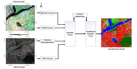
Feature-Level Fusion of Polarized SAR and Optical Images Based on Random Forest and Conditional Random Fields

Abstract

In terms of land cover classification, optical images have been proven to have good classification performance. Synthetic Aperture Radar (SAR) has the characteristics of working all-time and all-weather. It has more significant advantages over optical images for the recognition of some scenes, such as water bodies. One of the current challenges is how to fuse the benefits of both to obtain more powerful classification capabilities. This study proposes a classification model based on random forest with the conditional random fields (CRF) for feature-level fusion classification using features extracted from polarized SAR and optical images. In this paper, feature importance is introduced as a weight in the pairwise potential function of the CRF to improve the correction rate of misclassified points. The results show that the dataset combining the two provides significant improvements in feature identification when compared to the dataset using optical or polarized SAR image features alone. Among the four classification models used, the random forest-importance_ conditional random fields (RF-Im_CRF) model developed in this paper obtained the best overall accuracy (OA) and Kappa coefficient, validating the effectiveness of the method.

1. Introduction

The impact of urban development on the Earth’s environment is enormous, leaving an ever-changing imprint on its surface. This situation calls for a compulsory requirement to map the land cover and review land-use patterns of our dynamic eco-system time [1]. Polarized Synthetic Aperture Radar (SAR) and optical image have gained many applications in land cover classifications [2,3,4,5]. Since the two have entirely different physical properties, this makes them have distinct advantages in classification. For example, the optical images are susceptible to differences in the vegetation spectrum and are, therefore, often used to detect pest and disease problems [6]. SAR images offer high accuracy and purity in detecting water areas, but extracting sharp edges is still a challenge [7]. Therefore, how to fully utilize the advantages of both is one of the major topics currently faced.

Data fusion is a way to take full advantage of multiple sources of data. The data fusion stages (pixel-level, feature-level, and decision-level) determine the data fusion techniques [8]. Feature-level fusion consists of two critical processes: image feature extraction and feature merging. In this regard, Aswatha et al. [1] used multimodal information from multispectral images and polarized SAR data to classify land cover into seven classes in an unsupervised manner. Su [9] extracted the backward scattering features and grey-level co-occurrence matrix (GLCM) features obtained from the Pauli decomposition and H/A/alpha decomposition of polarized SAR images, the spectral features, and GLCM features of multispectral images, and used a support vector machine (SVM) for classification. This fusion method effectively improves the classification accuracy and the pepper noise is reduced.

Land cover classification is one of the critical applications of remote sensing images. The traditional land cover classification method is divided into two steps: feature extraction and classifier training [10].

The feature extraction for optical images is based on spectral and textural features. A textural feature is a comprehensive reflection of the image greyscale statistical information, spatial distribution information, and structural information. Commonly used textural feature classification algorithms include a local binary pattern (LBP) [11], GLCM [12], etc. Polarized SAR feature extraction is based on polarized target decomposition, which aims to decode the scattering mechanism of the feature under a reasonable physical constraint model [13], such as Freeman-Durden decomposition [14], Yamaguchi decomposition [15], etc.

Machine learning has achieved considerable progress in classification and regression tasks. Commonly used machine learning is SVM, decision tree, random forest, etc. In the current research, SVM has been used extensively. For example, Attarchi [16] used SVM to classify polarized SAR data and its GLCM features for the detection of impervious surfaces. While SVM classifies samples by finding hyperplanes, decision trees classify samples by selecting the optimal components and dividing the subset into the corresponding leaf nodes based on the features. Phartiyal et al. [17] used an evolutionary genetic algorithm to optimize the empirical model to maximize the classification performance. They constructed a decision tree based on the best class boundary and obtained satisfactory classification results. Random forest is an ensemble learning model based on decision trees, which obtains the final results by combining and analysing multiple decision trees [18]. Du et al. [19] extracted the polarization and texture features of the fully polarized SAR images for random forest and rotation forest classifiers. The experiment finally verified that random forest is better than Wishart and SVM classifiers, and it is less accurate than rotation forest but faster.

In image processing, conditional random fields (CRF) have unique advantages in expressing the spatial context and the posterior probability modelling [20]. Zhong et al. [21] proposed the spatial-spectral-emissivity land-cover classification based on the conditional random fields (SSECRF) algorithm, which integrates the spatial-spectral feature set and emissivity by constructing the SSECRF energy function to obtain better classification results. CRF allows for the processing of target classes in conjunction with neighbourhood information, effectively improving the image purity of the classification results, which is missing from machine learning.

This article proposes an RF-Im_CRF classification model to improve the accuracy of the random forest classifier in feature-level fusion classification. The model first extracts the spectral and GLCM features of optical images, the Freeman decomposition, and Polarization Signature Correlation Feature (PSCF) features of polarized SAR. Then, the model assembled them into a random forest training dataset. Afterward, the random forest classifier results are input into the Im_CRF model, which uses the feature importance from the random forest as the weight information in the pairwise potential function to improve feature classification accuracy.

2. Materials

2.1. Study Site

The location selected for this study is in Nanjing and its surrounding area, which is located in Jiangsu Province in Eastern China. Figure 1 shows the optical and polarized SAR false-colour images of the study area. The false-colour image is generated based on the Pauli decomposition. The images are 1500 × 1500 pixels in size, which include river, buildings, vegetation, and roads. The image resolution is 8 metres, so the total size of the study area is about 169 km². The architective area occupies the majority of the image, the vegetation area is relatively concentrated, and there is a small amount of vegetation within the building space. The cultivated area is concentrated in the northern part of the river. A clear colour difference can be observed in the optical image between the dense vegetation area and the cultivated area. The colour of the river part is not sufficiently uniform, which is similar to the farmland in some areas. In contrast, the river area of the SAR false-colour image is different from other regions. Therefore, it can be seen that polarized SAR has apparent advantages in identifying river categories.

The dataset used for research is the polarized SAR data collected by the RADARSAT-2 satellite, which has four polarization states: HH, VV, HV, and VH. This data was acquired on 19 April 2011 at a resolution of 8 m. The optical image resolution is 5 m, and the acquisition time is April 2017. Due to the relatively low resolution and the fact that the acquisition time falls within the same month, the variation in ground objects is within manageable limits. In the ENVI software, the optical image was down-sampled to a resolution of 8 m, and the polarized SAR image has undergone preprocessing such as multi-looking and noise reduction. The two images were calibrated in the same geographic coordinate system.

2.2. Sampling Point Selection

The sampling point coordinates in the experiment were taken with the optical image as a reference. Overall, five land cover categories were considered, namely Water, Building, High vegetation, Low vegetation, and Road. The high vegetation is dominated by tall forests and the low vegetation is dominated by agricultural land. Since the image resolution is 8 m, this prevents some narrow roads from being clearly represented, especially for SAR images. This paper, therefore, chose to sample roads with larger width, such as motorways and arterial roads. Because of the massive amount of source image data, it is not easy to classify the entire image finely. Therefore, the training samples chosen for this experiment are 100 per class, and the test samples are 150 for each category, as shown in

Table 1. Sample label type and quantity.

Label Category	Train Number	Test Number
Water	100	150
High vegetation	100	150
Building	100	150
Low vegetation	100	150
Road	100	150
Total	500	750

. The totals of training samples and test samples are 500 and 750, respectively, with no duplicate points.

3. Characteristic Data Acquisition

3.1. Polarization Feature Extraction

For the extraction of polarized SAR image features, this experiment selected two polarization feature extraction methods known as the Freeman-Durden decomposition and the PSCF.

3.1.1. Freeman-Durden Decomposition

The Freeman-Durden polarization decomposition method is based on the fundamental principle of radar scattering, which decomposes the SAR cross-covariance matrix into canopy scattering (or volume scattering), odd bounce scattering (or surface scattering), and double-bounce scattering (or dihedral scattering). The detailed description of the modelling process for the composite scattering model can be found in Reference [22]. This model can acquire the characteristic parameters related to the three scattering mechanisms and the corresponding weight coefficients.

The power corresponding to the three scattering mechanisms are Ps, Pd, and Pv, where Ps corresponds to the power of surface scattering, Pd represents the power of dihedral scattering, and Pv represents the power of volume scattering. Then, the Freeman feature vector of the target points can be established.

$$X_{Freeman}={[x_i^{Pd},x_i^{Ps},x_i^{Pv}]}^T$$

(1)

3.1.2. Polarization Signature Correlation Feature (PSCF)

Radar polarization signatures (PSs) can effectively characterize the scattering behaviour of the research object, so it has the potential to distinguish the types of ground objects. This feature is usually a three-dimensional representation of the backscattering behaviour of a target or land cover. In the expression of PSs, the x-axis and y-axis represent the ellipse angle and azimuth angle, respectively, and the z-axis represents the received backscattering power coefficient. The value range of the azimuth angle ($\psi$) is −90 to 90 degrees, and the value range of the ellipse angle ($\chi$) is −45 to 45 degrees. The following formula gives the PSs.

$$\sigma \left({\chi }_i{\psi }_i{\chi }_j{\psi }_j\right)=\frac{4\pi }{k^2}\left(\begin{array}{c}1\\ \cos 2{\chi }_i\cos 2{\psi }_i\\ \cos 2{\chi }_i\sin 2{\psi }_i\\ \sin 2{\chi }_i\end{array}\right)\left(K\right)\left(\begin{array}{c}1\\ \cos 2{\chi }_j\cos 2{\psi }_j\\ \cos 2{\chi }_j\sin 2{\psi }_j\\ \sin 2{\chi }_j\end{array}\right)$$

(2)

Among them, $\sigma$ represents the backscattering coefficient or received power, the subscripts i and j mean the transmitting and receiving units, respectively, and K is the Kennaugh matrix [23]. $k$ is the wave number of the illuminating wave.

The co-polarized signatures are obtained by transmitting and receiving combination ${\psi }_i={\psi }_j,{\chi }_i={\chi }_j$, and the cross-polarized signatures are obtained by ${\psi }_i=90+{\psi }_j,{\chi }_i=-{\chi }_j$. The ellipse angle defines the polarization behaviour (linear polarization, circular polarization, or elliptical polarization), and the azimuth angle defines the polarization states, that is, horizontal or vertical polarization [24]. In the current research, the characteristics of co-polarized and cross-polarized signatures have been fully considered and utilized.

Since surface objects generally exhibit a complex scattering response, the polarization signatures of standard targets must be used as a reference for classification. Therefore, PSs have been calculated for flat plate (FP), horizontal dipole (HD), vertical dipole (VD), and a dihedral angle (Di) in the standard targets. The formulae for the generation of the standard target PSs are given in Reference [25].

Therefore, the PSCF uses the radar polarization signatures of the four standard scatterers (FP, HD, HD, and VD) as a reference to calculate the relevance between the polarization characteristics of the target points and the above four standard targets. This can be a reference to distinguish between different categories. The correlation coefficient formula is as follows.

$$CC=\frac{S_{xy}}{S_x{S}_y}$$

(3)

where x and y are the polarized characteristics of the target points and the standard targets, respectively. $S_x$ is the standard deviation of x, $S_y$ is the standard deviation of y, and $S_{xy}$ is the covariance between x and y. CC is the correlation coefficient between x and y.

This paper refers to Reference [17] to obtain the PSCF solution and establish the feature correlation coefficients between a single target and four standard targets, which are Corr_co_Di, Corr_co_FP, Corr_co_HD, Corr_co_VD, Corr_cross_Di, Corr_ cross _FP, Corr_ cross_HD, and Corr_ cross _VD. Among them, the co is for the co-polarization while the cross is for cross-polarization. Thus, the PSCF feature vector of the target point is established as:

$$\begin{gathered} X_{PSCF}=[x_i^{corr\_co\_Di},x_i^{corr\_co\_FP},x_i^{corr\_co\_HD},x_i^{corr\_co\_VD}, \\ {x}_i^{corr\_cross\_Di},x_i^{corr\_cross\_FP},x_i^{corr\_cross\_HD},x_i^{corr\_cross\_VD}{]}^T \end{gathered}$$

(4)

3.2. Optical Image Feature Extraction

3.2.1. Spectral Information Extraction

Compared with multispectral images, the optical image does not have rich spectral information, but it is also sufficient to identify information with significant spectral differences. This optical image can be divided into three bands: red, green, and blue, so the spectral feature information is shown as follows.

$$X_{Spectral}={[x_i^r,x_i^g,x_i^b]}^T$$

(5)

3.2.2. Grey-Level Co-Occurrence Matrix (GLCM)

The textural feature is a visual feature that does not depend on brightness and colour, reflecting similar information of adjacent pixels in the image. It reflects the internal characteristics shared by the surface of the object. It contains essential information about the surface structure of the object and the relationship to its neighbours.

GLCM is a commonly used method for extracting texture information with good discrimination ability. Its principle is to convert the specified spatial relationship in the image into texture information based on the greyscale value. The texture features obtained by GLCM are helpful to distinguish objects with similar spectral characteristics.

In this paper, three features are chosen to describe the spatial relationships of images: contrast, dissimilarity, and energy. Contrast and dissimilarity can measure the local variation and reflect the sharpness of the image and the depth of the texture. The energy is the sum of the squares of element values of the GLCM, demonstrating the uniformity of the image greyscale distribution and the texture thickness. The GLCM feature information is expressed as follows.

$$X_{GLCM}={[x_i^{contrast},x_i^{dissimiliraty},x_i^{energy}]}^T$$

(6)

4. Random Forest-Importance_Conditional Random Forest (RF-Im_CRF) Model

Figure 2 is the flowchart of applying the RF-Im_CRF model to the feature-level fusion of polarized SAR and optical images. After extracting the features of the two images, the random forest is first used for classification. Then, the classification results and feature importance of the random forest are combined with the CRF. The classification results are taken as the unary potential function and the feature importance is taken as the weight of the pairwise potential function to improve the classification accuracy.

4.1. Random Forest

Random forests construct mutually independent decision trees in which each generates a training set by bootstrap resampling. M rounds were randomly selected from the original training set with N samples to obtain M training sets. Some samples may be chosen multiple times under self-service resampling, while some samples may not be drawn. Then M decision trees are developed according to these training sets. In the decision-making stage, the classification results are obtained by taking the mode, or the regression results, by taking the average value. The random forest can process large data sets with high efficiency and precision, filter explanatory variables by itself, and get the mutual influence and importance ranking of variables.

The Gini index, or Gini impurity, indicates the probability that a randomly selected sample in the sample set will be misclassified. At each node in the binary tree T of the random forest, the optimal segmentation is sought according to the Gini index $i(\tau )$, which divides the sub-node data set. Random forest follows the principle of Gini gain maximization when selecting features for nodes [26]. Let $p_k$ be the probability of node $\tau$ being divided into child nodes ${\tau }_k,k=1,2$. Then the Gini index is:

$$i\left(\tau \right)={\displaystyle \sum }_{k=1}^2{p}_k\left(1-p_k\right)=1-{\displaystyle \sum }_{k=1}^2{p}_k^2$$

(7)

The Gini gain $\Delta i$ generated by splitting the sample through a certain threshold and sending it to two child nodes ${\tau }_1$ and ${\tau }_2$, which is defined as:

$$\mathsf{\Delta }i\left(\tau \right)=i\left(\tau \right)-p_{1}i\left({\tau }_1\right)-p_{2}i\left({\tau }_2\right)$$

(8)

Since the decision tree selects features that can maximize the Gini gain of the node when generating nodes, the feature importance can be reflected by the sample division of the nodes. However, random forest introduces the double randomness of data samples and input features during a training process, which may cause important features with high discrimination being used to divide nodes less frequently than features with low discrimination. Therefore, the importance of features cannot be measured simply by the number of times used as segmentation attributes [27,28].

4.2. Conditional Random Fields

The CRF model simulates the local neighbourhood interaction between random variables in the unified probability framework. Given the observed image data, the model directly models the posterior probability of the label as a Gibbs distribution.

The general form of the CRF model is:

$$P\left(Y|X\right)=\frac{1}{Z\left(X\right)}exp\left\{-\left[{\displaystyle \sum }_{i\in V}{\Phi }_i\left(y_i,x_i,w\right)+\beta {\displaystyle \sum }_{\left(i,j\right)\in E}{\Phi }_{ij}\left(y_i,y_j,x_i,x_j,v\right)\right]\right\}$$

(9)

Among them, $V$ is for the set of data points and $E$ is for the set of point neighbours.

$x_i$, $y_i$ represents the observation variable of the $i$-th point in the data and its class label variable, respectively. $X$ is the sequence of observations,$X=\left[x_1,\dots ,x_i,\dots ,x_N\right]$. $Y$ is the sequence of tags corresponding to $X$, $Y=\left(y_1,\dots ,y_i,\dots ,y_C\right)$, where $C$ is the number of categories. $P\left(Y|X\right)$ is the probability of the label sequence $Y$ under the given observation sequence $X$. $Z\left(X\right)$ is the normalization constant, $Z\left(X\right)=\sum _{Y}exp\left\{-\sum _{c\in C}{\Phi }_c\left(y_c,x\right)\right\}$; ${\Phi }_i(\cdot )$ is the unary potential function, which represents the probability of the observed variable $x_i$ taking the label $y_i$. ${\Phi }_{ij}(\cdot )$ is the pairwise potential function, which means the correlation between the variable $x_i$ and its neighbouring variables $x_j$ and the correlation between the labels. $w$, $v$, respectively, represents the parameters of the correlation potential function and the interaction potential function. $\beta$ is to adjust the weight of the two potential function terms, which determines the degree of influence of the pairwise function on the unray potential function. In this article, to simplify the implementation of CRF, $\beta$ is set to a constant 1.

Then the corresponding Gibbs energy is defined as:

$$\begin{gathered} E\left(Y|X\right)=-\log P\left(Y|X\right)-\log (Z\left(X\right))={\displaystyle \sum }_{c\in C}\Phi \left(y_c,x\right) \\ ={\displaystyle \sum }_{i\in V}{\Phi }_i\left(y_i,x_i,w\right)+\beta {\displaystyle \sum }_{\left(i,j\right)\in E}{\Phi }_{ij}\left(y_i,y_j,x_i,x_j,v\right) \end{gathered}$$

(10)

According to the Bayesian Maximum Posterior (MAP) rule, image classification aims to find the label Y that maximizes the posterior probability $P\left(Y|X\right)$. Therefore, the CRF’s MAP mark xMAP can be obtained by the following formula.

$$Y_{MAP}=arg \underset{y}{max }P\left(Y|X\right)=arg \underset{y}{min }E\left(Y|X\right)$$

(11)

It can be seen that finding the maximum value of the posterior probability $P\left(Y|X\right)$ is equivalent to finding the minimum value of the energy function $E(Y|X)$. Therefore, the optimization algorithm finds the most probable label by finding the minimum energy solution.

4.3. RF-Im_CRF Model

4.3.1. Establishment of Potential Functions

In this paper, the unary potential function ${\Phi }_i$ is defined based on the classification results of the random forest classifier. For variables $x_i$ and its label $y_i$, when $y_i=k$, $\forall k\in K$ (K is the label set), then Equation (12) is:

$$P\left(y_i=k|x_i\right)=\frac{1}{M}{\displaystyle \sum }_{m=1}^M\delta \left[T_m\left(x_i,{\theta }_m\right)=k\right]$$

(12)

M is the total number of decision trees. ${\theta }_m$ is the independent and identically distributed parameter vector describing the m-th decision tree. Then, $P\left(y_i=k|x_i\right)$ represents the probability that the target is of class $k$.

The CRF unary potential function is defined as:

$${\Phi }_i\left(y_i,x_i\right)=-logP\left(y_i|x_i\right)$$

(13)

Pairwise potential function ${\Phi }_{ij}\left(y_i,y_j,x_i,x_j,v\right)$, also called the smoothness term, encourages adjacent pixels of the image to use the same label. This article uses an improved contrast-sensitive Potts model that introduces the feature importance ${\eta }_k$ to define the pairwise potential function.

$${\Phi }_{ij}\left(y_i,y_j,x_i,x_j\right)=\{\begin{array}{cc}0& if y_i=y_j\\ g_{ij}\left(S\right)& otherwise\end{array}$$

(14)

$$g_{ij}\left(S\right)=dist{\left(i,j\right)}^{-1}exp\left(-{\displaystyle \sum }_{k=1}^N{\eta }_k{\gamma }_k\parallel X_i^k-X_j^k\parallel {}^2\right)$$

(15)

Among them, $g_{ij}$ simulates the spatial interaction of adjacent pixels $x_i$ and $x_j$, which is used to measure the feature difference between neighbours. $dist\left(i,j\right)$ is the Euclidean distance between adjacent pixels, $X_i^k$ and $X_j^k$ represent the feature vector between points $i$ and $j$. $k$ represents the category of the feature vector, namely, $k=1,2,3,4$, which, respectively, represents the feature vector $X_{Freeman},X_{PSCF},X_{Spectral},X_{GLCM}$. ${\gamma }_k$ is set to be the mean square error of feature vectors between adjacent pixels in the image, denoted as ${\gamma }_k={\left(2⟨\left|\right|X_i^k-X_j^k\left|\right|{}^2⟩\right)}^{-1}$, which $\langle \cdot \rangle$ represents the mean value of the neighbourhood. The parameter ${\eta }_k$ is the feature importance in the classification process, obtained by random forest.

4.3.2. Feature Importance

In this paper, the statistic ${\mathrm{Im}}_i^{}$ is used as a feature importance measurement based on the Gini index, representing the average change in the Gini index of the i-th feature in the node division of all decision trees. The importance of feature $x_i$ on node n is the change in the Gini index that the sample on the node $\tau$ is divided into child nodes ${\tau }_1$ and ${\tau }_2$ in which:

$$I{m}_{i,m,n}=i\left(\tau \right)-i\left({\tau }_1\right)-i\left({\tau }_2\right)$$

(16)

where $n=1,\dots ,N$, which represents the node index in one decision tree, and $m=1,\dots ,M$, which represents the decision tree index in the random forest. Therefore, the feature $x_i$ has N nodes in the m-th decision tree as the attribute of node division. Then the feature importance $x_i$ on this decision tree can be expressed as:

$$I{m}_{i,m}={\displaystyle \sum }_{n=1}^{N}I{m}_{i,m,n}$$

(17)

The feature importance $x_i$ in the entire random forest is:

$$I{m}_i=\frac{1}{M}{\displaystyle \sum }_{m=1}^{M}I{m}_{i,m}$$

(18)

The sum of the feature importance of each feature is 1.

For parameter ${\eta }_k$, Freeman decomposition, PSCF features, spectral features, and GLCM features are regarded as four various feature components. Then, taking spectral features as an example, the feature importance of this characteristic component is:

$${\eta }_{Spectral}=I{m}_r+I{m}_g+I{m}_b$$

(19)

The four feature components extracted in this paper have different value ranges and number of elements. Since the normalization of features does not affect the random forest results, they are not normalized in feature extraction. However, in the CRF, this difference in the value range affects the pairwise potential function. Therefore, it needs to be divided into four parts to avoid the features with a small value range in which they do not work as well as they should. Since the importance of each feature is different, the higher the importance of the feature, the greater the influence on classification. Therefore, the parameters ${\eta }_k$ can further strengthen the feature difference between neighbours and improve classification accuracy.

5. Experiment and Analysis

5.1. Multi-Source Data Comparative Classification Experiment

First, to verify the advantages of image fusion in image classification, this paper used the random forest to perform classification experiments on optical image data and polarized SAR data. The optical image data contains a feature vector consisting of spectral and GLCM information, and the polarized SAR data includes a feature vector consisting of Freeman and PSCF information. The number of decision trees in the random forest was set to 100. This value ensures that the results of the random forest will be optimal and fluctuate within a range of values. The experimental results are shown as follows.

For classification tasks, the classification results can intuitively and clearly reflect the disparity between different features or different classification methods, especially when the distinction is significant. Figure 3 shows the classification results obtained by adopting different feature vectors. It can be seen that the characteristics of the optical image can better distinguish the difference between high and low vegetation due to the apparent differences in spectra. However, the reliance on spectral features also makes many errors in the identification of waters. Since the water surface tends to be specularly reflective, the backscatter from the water surface is almost zero, resulting in high accuracy of SAR image classification in waters. At the same time, the working frequency band of RADARSAT-2 is C-band, which has certain penetrability, making it difficult to distinguish the characteristic difference between high and low vegetation, thus, presenting a mixed phenomenon of dark green and light green. This penetrability is also reflected in the ability of the polarized SAR data to detect folds in the hills and present similar features to buildings, leading to misinterpretations. Optical image features have certain advantages in terms of buildings, and it is difficult for both sides to get ideal results on the road.

The visual effect of the classification that combines polarized SAR and optical image features is significantly improved. The water area as well as high and low vegetation are well inherited. Simultaneously, compared with the former two, the salt and pepper noise in the construction area has been significantly reduced. The large area of misjudgment is also hard to see, and the display effect of the road is improved. This indicates that the characteristics of polarized SAR and optical images both play a specific role in classification. Due to the similarity of the narrow river sections to the backscattering of the road, this caused the SAR data to misinterpret at the river in the southwest region of the image. This situation is also shown in Figure 3c. This indicates that the features of the optical images are still difficult to correct for the high misclassification of SAR images in this particular scene.

From the experimental results, it can be seen that the integrated polarized SAR and optical image fusion classification performance is significantly improved compared with the image classification performance of the single source. However, there are still many noise points, which affect the smoothness of the classification result. The RF-Im_CRF model proposed in this paper will improve the classification results aiming at this phenomenon.

5.2. Comparison of RF-Im_CRF Model Experiment Results

5.2.1. Analysis of Classified Image Results

To verify the effectiveness of the algorithm in this paper, the experimental data were classified using SVM based on Poly kernel function, RF, RF-CRF without feature importance as weights [21], and the RF-Im_CRF models, respectively. The experimental data is the feature vector composed of the four features in Chapter 3 of the article. The results are shown in Figure 4.

It can be seen that the SVM has the worst classification effect. SVM is an independent classifier, so it follows one rule when classifying. Random forests, on the other hand, rely on multiple mutually independent decision trees acting together, each with a different classification threshold. This means that the misclassification results of a single decision tree are corrected by the action of other decision trees. As a result, random forests give better results.

Compared with the random forest classifier, the RF-CRF model significantly improves image smoothness, since the CRF eliminates most salt and pepper noise. The differences between the RF-CRF and RF-Im_CRF models are difficult to see. Therefore, this paper extracted three scenes in the image for comparison to show the performance gap between the two models. The reference data are the optical image and the real classification results based on the optical image.

As shown in Figure 5, when compared with the RF-CRF model, the RF-Im_CRF model can further reduce the salt and pepper noise in the image, and the smoothness can be further improved. Since parking lots are set up around some large buildings, the classifier will be difficult to balance between roads and buildings. Some open places such as sports fields and squares as well as roads have more white blocks in area 1, which represent the road. Area 2 has lower category complexity and better homogeneity of vegetation, so there is less variation in the effects of classification. There are narrow roads in area 3, which were not sampled as samples during the sampling process, since it hardly distinguished with low contrast between neighbours in the SAR image. Therefore, it is misclassified as low vegetation in the classification result. The small white areas in the river are the ships sailing on the river in the SAR image. The RF-Im_CRF model is better than the RF-CRF model in identifying the riverbank portion on the left side, showing a relatively complete low vegetation zone.

The display of the classification results shows that, when compared with the RF-CRF model, the RF-Im_CRF further improves the classification accuracy, resulting in less noisy images and a further increase in purity. This is because the value range of various features is diverse. For example, the value range of the spectral feature is between 0–255, while the value range of PSCF is between -1 and 1. The feature difference is calculated in the unit of a feature component in CRF, which helps reduce the overall influence of features with a wide value range. Simultaneously, after adding feature importance as weights, the impact of features with high importance on feature differences between neighbours is enhanced. Therefore, the RF-Im_CRF model can classify ground objects more accurately.

5.2.2. Classification Data Analysis

This paper quantified the classification effectiveness of the classification model through Overall Accuracy (OA) and a Kappa coefficient, and analysed various classification cases using precision and recall.

When the training set is the same, the SVM produce the same results in multiple experiments. In contrast, the random forest has a certain degree of randomness. Even though the training set is the same, the results obtained during each training set are different. Therefore, we used the same dataset for ten consecutive tests on the random forest model to get the average of the results. In each experiment, the RF, RF-CRF, and RF-Im_CRF models use the same RF model results, which are only different in the subsequent processing. The RF model was built on Scikit-learn package using Python [29]. In each experiment, this paper extracted the feature importance and the probability of each class of all points. At the end, the evaluation index, such as OA and Kappa coefficients, were obtained for each model based on classification results.

The OA, Kappa values, and their 95% confidence interval are shown in

Table 2. The average of OA and Kappa.

	SVM	RF	RF-CRF	RF-Im_CRF
OA	79%	88.0%	91.6%	94.0%
95% confidence interval		[85.88%,90.4%]	[90.22%,93.02%]	[93.52%,94.54%]
Kappa	0.74	0.85	0.89	0.91
95% confidence interval		[0.834,0.866]	[0.879,0.905]	[0.902,0.918]

.

With the same test data and constant parameters, the results of the SVM are always consistent and, therefore, there are no confidence intervals. In terms of a quantitative data comparison, the RF-Im_CRF model proposed in this paper has the best classification accuracy with an average OA of 94.0%, and the 95% confidence interval is [93.52%,94.54%]. The Kappa coefficient is 0.91 with the 95% confidence interval of [0.902,0.918]. Compared with SVM, RF, and RF-CRF, OA increased by 15%, 6%, and 2.4%, respectively, and classification reliability increased by 17%, 6%, and 2%, respectively. The reason is that SVM and RF classify single pixels, which are inevitably misclassified even with the inclusion of textural information. CRF can use neighbourhood information to correct misclassified pixels, thereby, improving the classification accuracy. The comparison of the above results shows that the RF-Im_CRF model can further significantly reduce the noise generated in the random forest classification and improve the smoothness of images due to the correction capability of Im_CRF.

In order to analyse the classification accuracy relationship between each category, we give the experimental result data obtained in a single experiment, as shown in

Table 3. Comparison of results of different classifiers.

Model		Water	High	Building	Low	Road
	Precision (%)	87	85	72	79	74
	Recall (%)	77	88	84	84	63
	F1-score (%)	82	86	78	81	70
RF	Precision (%)	98	92	79	85	78
	Recall (%)	95	93	91	81	72
	F1-score (%)	96	92	85	83	75
RF-CRF	Precision (%)	99	96	80	90	82
	Recall (%)	95	95	93	88	75
	F1-score (%)	97	95	86	89	78
RF-Im_CRF	Precision (%)	100	97	84	93	88
	Recall (%)	95	96	97	89	84
	F1-score (%)	97	96	90	91	86

. In the absence of CRF, the 95% confidence interval of each class of random forest is basically between $[A+2\%,A-2\%]$. Where $A$ represents the classification accuracy of each category. The Bootstrap Resampling method of the random forest causes each decision tree to use a different training subset, which leads to differences in classification performance across the trees. With a large number of decision trees, the random forest itself is more accurate than the SVM method, but it inevitably generates randomness, which results in slightly different classification results for each category. The number of test sets for each category is 150, which means that there are three different classification results for this category in the two experiments, and there will be a 2% difference.The classification effect is further improved by the CRF, resulting in a 95% confidence interval between $[A+1\%,A-1\%]$.

It can be seen that the four models are more accurate in classifying water, high vegetation, and low vegetation than buildings and roads. The reason is that buildings have high complexity in both spectrum and structural characteristics, while roads are more challenging to identify due to low image resolution, a narrow area, and a susceptibity to factors, such as street trees. Among the two, roads are the most difficult to identify and the most error-prone category. This is because roads are mostly between buildings including the boundary between the road and the building that will blur the road with low image resolution. Moreover, the backscattering characteristics of buildings in SAR image can obscure the road to a certain extent, which has a negative impact on classification and makes roads more likely to be misclassified as buildings. At the same time, in the mixed area of multi-category features, low-resolution images significantly increase the complexity of categories, which makes the boundaries between categories difficult to distinguish. Therefore, how to effectively select feature quantities or improve image resolution to enhance the classification effect of buildings and roads, and make more precise distinctions to mixed regions will become the following research focus.

In terms of the model’s operational efficiency, since the model proposed in this work needs to use neighbourhood information, this means that neighbourhood pixels must be classified as well. On the contrary, the original random forest classifier does not need to classify neighbourhood pixels. Therefore, the computational amount in the calculation process for this model is significantly higher than the one required for simpler classifiers, such as SVM or random forest. The evaluation of computing efficiency and the possible improvements of the algorithm from the computational point-of-view are in progress and will be the subject of the follow-up work.

5.2.3. Analysis of Feature Importance

This article also extracted the feature importance of each feature vector in the above ten experiments and took the average to get the results shown below.

As shown in

Table 4. Feature importance of four characteristic components.

Feature	Freeman	Spectral	GLCM	PSCF
$\eta$ (%)	33.78	30.03	13.44	22.72

and

Table 5. Feature importance of each feature.

Class	Pd	Ps	Pv	R	G	B	G1	G2	G3	P1	P2	P3	P4	P5	P6	P7	P8
$Im$ (%)	7.35	5.91	20.53	8.94	9.15	11.96	3.11	2.84	7.49	3.93	2.93	2.14	2.01	3.95	2.30	2.74	2.74

G₁ = contrast, G_-2 = dissimilarity, G₃ = energy, P₁ = Corr_co_Di, P₂ = Corr_co_FP, P₃ = Corr_co_HD, P₄ = Corr_co_VD, P₅ = Corr_cross_Di, P₆ = Corr_cross_ FP, P₇ = Corr_cross_ HD, P₈ = Corr_cross_VD.

and Figure 6, the feature importance of Freeman decomposition and spectral features are higher than others in the random forest classification. For the individual feature vectors, the volume scattering component in Freeman decomposition has the highest feature importance, which is followed by the blue component of spectral features. Nevertheless, the difference between the components of the spectral characteristics is not significant. This is because the volume scattering component is generally higher in the Freeman decomposition than the surface scattering and dihedral scattering for all targets except water. In water targets, these three components are small, and the scattering properties of road targets are similar to water under ideal conditions. Therefore, the volume scattering component has a good basis for judging the water area or road. Therefore, the body scattering has the highest feature importance. The recognition rate is not as ideal in water areas because of the complex and narrow environment in which roads are located.

Except for energy, the GLCM and PSCF have similar proportions, while PSCF components are higher, so the $\eta$ value is relatively high. The feature importance reflects the contribution degree of each feature in the classification. The randomness of random forest also impacts the feature importance. Therefore, the 95% confidence interval of four characteristic components is between [A−1%, A+1%]. Using such a contribution degree as the weight in the CRF pairwise potential function clarifies the spatial relationship between the target and the neighbourhood and improves classification accuracy.

6. Conclusions

Relying on the unique advantages of CRF in spatial context feature modelling and classification, this paper established a pixel-based RF-Im_CRF model for classification based on various feature information, such as spectrum, texture, and polarization. The experiments and analyses were carried out using polarized SAR and optical images of Nanjing area as data. The results show that the fusion of multi-source image data improves the classification accuracy. The RF-Im_CRF model with multiple features proposed in this paper further improves the classification accuracy to more than 94%, which increases by 6% when compared with the random forest classifier. Therefore, the RF-Im_CRF model has good performance in the fusion classification of polarized SAR and optical images and can be used as a fusion classification method for heterogeneous images.

References

1. Aswatha, S.M.; Mukherjee, J.; Biswas, P.K.; Aikat, S. Unsupervised classification of land cover using multi-modal data from mul-ti-spectral and hybrid-polarimetric SAR imageries. Int. J. Remote Sens. 2020, 41, 5277–5304. [Google Scholar] [CrossRef]
2. Hall, D.K.; Riggs, G.A.; Salomonson, V.V. Development of methods for mapping global snow cover using moderate resolution imaging spectroradiometer data. Remote Sens. Environ. 1995, 54, 127–140. [Google Scholar] [CrossRef]
3. Wu, J.; Zhang, Q.; Li, A.; Liang, C.Z. Historical landscape dynamics of Inner Mongolia: Patterns, drivers, and impacts. Landsc. Ecol. 2015, 30, 1579–1598. [Google Scholar] [CrossRef]
4. Useya, J.; Chen, S. Exploring the Potential of Mapping Cropping Patterns on Smallholder Scale Croplands Using Sentinel-1 SAR Data. Chin. Geogr. Sci. 2019, 29, 626–639. [Google Scholar] [CrossRef] [Green Version]
5. Neetu; Ray, S.S. Evaluation of different approaches to the fusion of Sentinel -1 SAR data and Resourcesat 2 LISS III optical data for use in crop classification. Remote Sens. Lett. 2020, 11, 1157–1166. [Google Scholar] [CrossRef]
6. Malthus, T.J.; Madeira, A.C. High resolution spectroradiometry: Spectral reflectance of field bean leaves infected by Botrytis fabae. Remote Sens. Environ. 1993, 45, 107–116. [Google Scholar] [CrossRef]
7. Sun, J.; Mao, S. River detection algorithm in SAR images based on edge extraction and ridge tracing techniques. Int. J. Remote Sens. 2011, 32, 3485–3494. [Google Scholar] [CrossRef]
8. Pohl, C.; Genderen, J.L. Review Article Multisensor Image Fusion in Remote Sensing: Concepts, Methods and Applications. Int. J. Remote Sens. 1998, 19, 823–854. [Google Scholar] [CrossRef] [Green Version]
9. Su, R.; Tang, Y. Feature Fusion and Classification of Optical-PolSAR Images. Geomat. Spat. Inf. Technol. 2019, 42, 51–55. [Google Scholar]
10. Zhang, L.; Zou, B.; Zhang, J.; Zhang, Y. Classification of Polarimetric SAR Image Based on Support Vector Machine Using Multiple-Component Scattering Model and Texture Features. EURASIP J. Adv. Signal Process. 2010, 2010, 960831. [Google Scholar] [CrossRef] [Green Version]
11. Ojala, T.; Pietiainen, M.; Harwood, D. A Comparative Study of Texture Measures with Classification Based on Feature Distributions. Pattern Recognit. 1996, 29, 51–59. [Google Scholar] [CrossRef]
12. Haralick, R.M.; Shanmugam, K.; Dinstein, I. Textural Features for Image Classification. In IEEE Transactions on Systems, Man, and Cybernetics; IEEE: New York, NY, USA, 1973; Volume SMC-3, pp. 610–621. [Google Scholar] [CrossRef] [Green Version]
13. Dong, J. Statistical Analysis of Polarization SAR Image Features and Research on Classification Algorithm; Wuhan University: Wuhan, China, 2018. [Google Scholar]
14. Freeman, A.; Durden, S.L. A three-component scattering model for polarimetric SAR data. IEEE Trans. Geosci. Remote Sens. 1998, 36, 963–973. [Google Scholar] [CrossRef] [Green Version]
15. Sato, A.; Yamaguchi, Y.; Singh, G.; Park, S.E. Four-Component Scattering Power Decomposition with Extended Volume Scattering Model. IEEE Geosci. Remote Sens. Lett. 2012, 9, 166–170. [Google Scholar] [CrossRef]
16. Attarchi, S. Extracting impervious surfaces from full polarimetric SAR images in different urban areas. Int. J. Remote Sens. 2020, 41, 4644–4663. [Google Scholar] [CrossRef]
17. Phartiyal, G.S.; Kumar, K.; Singh, D. An improved land cover classification using polarization signatures for PALSAR 2 data. Adv. Space Res. 2020, 65, 2622–2635. [Google Scholar] [CrossRef]
18. Breiman, L. Manual on Setting Up, Using, and Understanding Random Forests V3.1 [EB/OL]; Statistics Department University of California Berkley: Berkley, CA, USA, 2002. [Google Scholar]
19. Du, P.; Samat, A.; Waske, B.; Liu, S.; Li, Z. Random Forest and Rotation Forest for fully polarized SAR image classification using po-larimetric and spatial features. ISPRS J. Photogramm. Remote Sens. 2015, 105, 38–53. [Google Scholar] [CrossRef]
20. Sutton, C.; Mccallum, A. An Introduction to Conditional Random fields. Found. Trends Mach. Learn. 2010, 4, 267–373. [Google Scholar] [CrossRef]
21. Zhong, Y.; Jia, T.; Ji, Z.; Wang, X.; Jin, S. Spatial-Spectral-Emissivity Land-Cover Classification Fusing Visible and Thermal Infrared Hyperspectral Imagery. Remote Sens. 2017, 9, 910. [Google Scholar] [CrossRef] [Green Version]
22. Wang, L.; Zhou, X.; Zhu, X.; Dong, Z.; Guo, W. Estimation of biomass in wheat using random forest regression algorithm and remote sensing data. Crop J. 2016, 4, 212–219. [Google Scholar] [CrossRef] [Green Version]
23. Harold, M. The Kennaugh matrix. In Remote Sensing with Polarimetric Radar, 1st ed.; John Wiley & Sons: Hoboken, NJ, USA, 2007; pp. 295–298. [Google Scholar]
24. Lee, J.S.; Grunes, M.R.; Boerner, W.M. Polarimetric property preservation in SAR speckle filtering. In Proceedings of SPIE 3120, Wideband Interferometric Sensing and Imaging Polarimetry; Mott, H., Ed.; SPIE: San Diego, CA, USA, 1997; pp. 1–7. [Google Scholar]
25. Lee, J.S.; Pottier, E. Electromagnetic vector scattering operators. In Polarimetric Radar Imaging: From Basics to Applications, 1st ed.; Thompson, B.J., Ed.; CRC Press: New York, NY, USA, 2009; pp. 92–98. [Google Scholar]
26. Menze, B.; Kelm, B.; Masuch, R.; Himmelreich, U.; Bachert, P.; Petrich, W.; Hamprecht, F. A comparison of random forest and its Gini importance with standard chemometric methods for the feature selection and classification of spectral data. BMC Bioinform. 2009, 10, 213. [Google Scholar] [CrossRef] [PubMed] [Green Version]
27. Altmann, A.; Toloşi, L.; Sander, O.; Lengauer, T. Permutation importance: A corrected feature importance measure. Bioinformatics (Oxf. Engl.) 2010, 26, 1340–1347. [Google Scholar] [CrossRef] [PubMed]
28. Strobl, C.; Boulesteix, A.L.; Kneib, T.; Augustin, T.; Zeileis, A. Conditional variable importance for random forests. BMC Bioinform. 2008, 9, 307. [Google Scholar] [CrossRef] [PubMed] [Green Version]
29. Pedregosa, F.; Varoquaux, G.; Gramfort, A.; Michel, V.; Thirion, B.; Grisel, O.; Blondel, M.; Prettenhofer, P.; Weiss, R.; Dubourg, V.; et al. Scikit-learn: Machine Learning in Python. J. Mach. Learn. Res. 2011, 12, 2825–2830. [Google Scholar]
Figure 1. Study area. (a) The optical image. (b) The polarized SAR false-colour image.
Remotesensing 13 01323 g001
Figure 2. RF-Im_CRF model flowchart.
Remotesensing 13 01323 g002
Figure 3. Multi-source data classification results. (a) Optical image classification result. (b) Polarized SAR classification result. (c) Optical + polarized SAR image classification result.
Remotesensing 13 01323 g003
Figure 4. Classification results with different classifier (a) SVM classifier result, (b) RF classifier result, (c) RF-CRF model result, and (d) RF-Im_CRF model result.
Remotesensing 13 01323 g004
Figure 5. Sub-area classification results. The regions numbered 1, 2, and 3 are the corresponding subregions in Figure 1a.
Remotesensing 13 01323 g005
Figure 6. Feature importance ring graph.
Remotesensing 13 01323 g006