
The Value of L-Band Soil Moisture and Vegetation Optical Depth Estimates in the Prediction of Vegetation Phenology


Abstract
:
1. Introduction
2. Materials
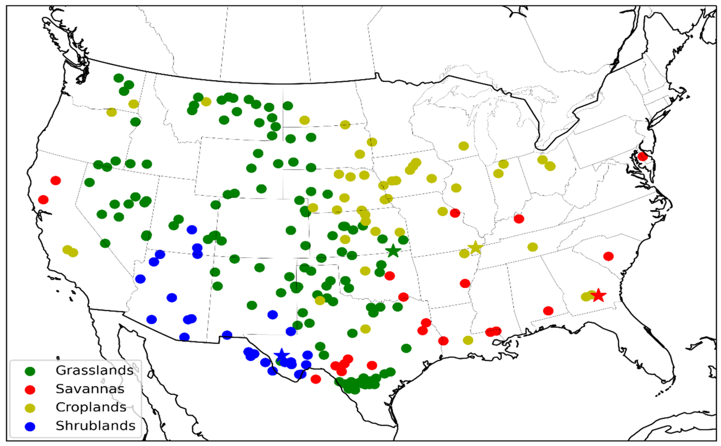
2.1. Study Sites
2.2. LAI Datasets
2.3. Landcover Information
2.4. Grid-Scale Geophysical Data
2.5. L-Band Microwave Data
3. Methodology
3.1. Shannon’s Entropy and Mutual Information
3.2. Random Forest Regression
4. Results
4.1. Input Dataset Characteristics
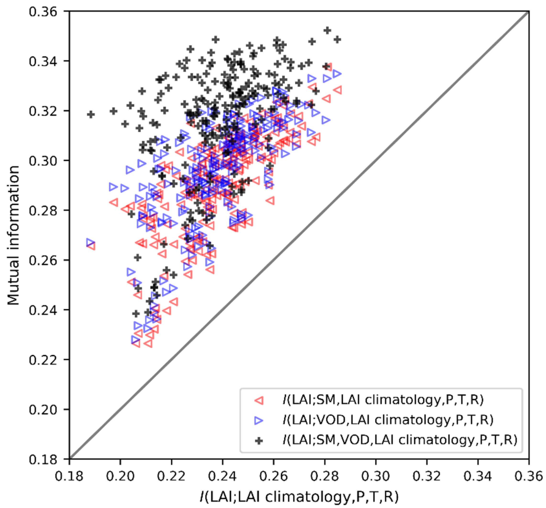
4.2. Mutual Information Analysis
4.3. LAI Anomaly Estimations
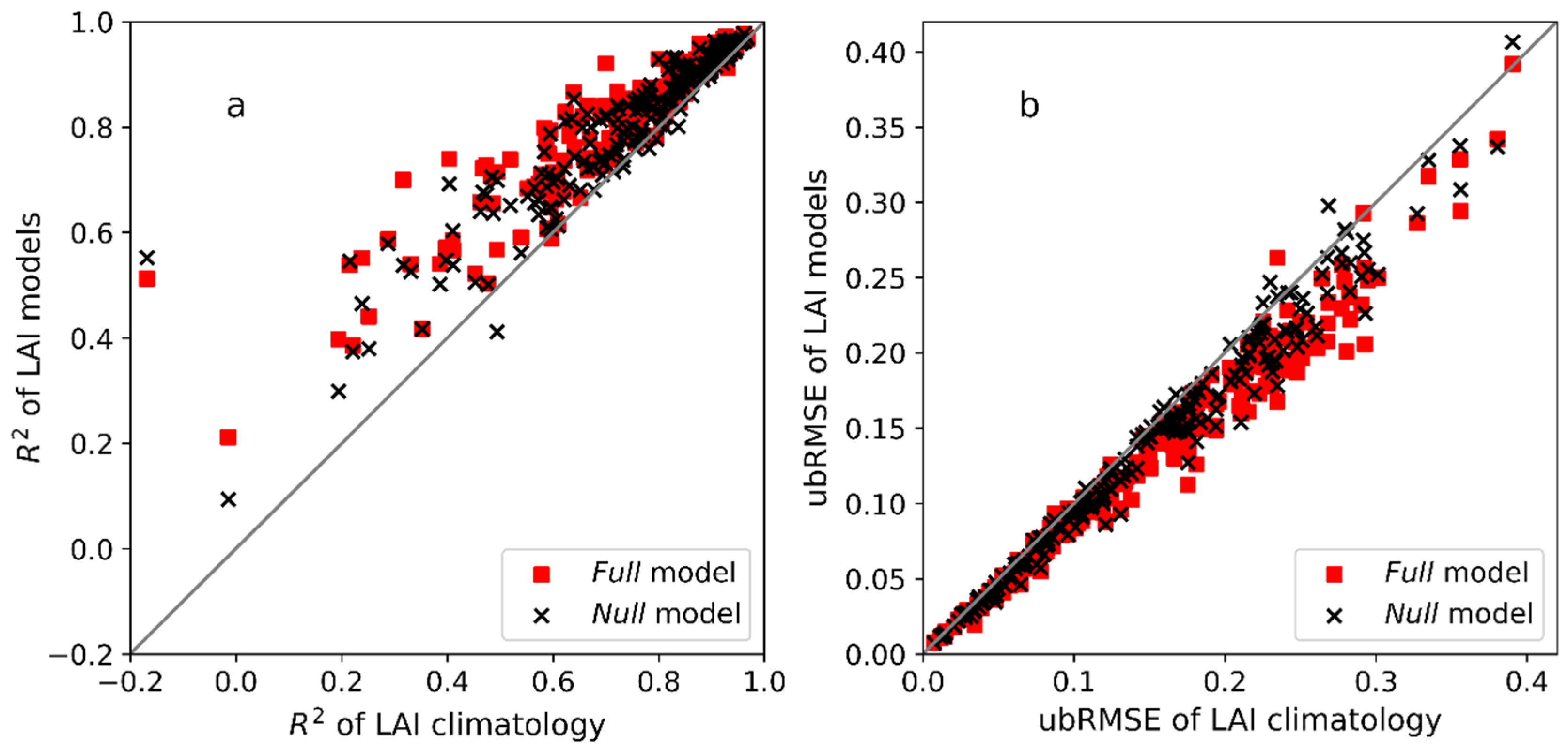
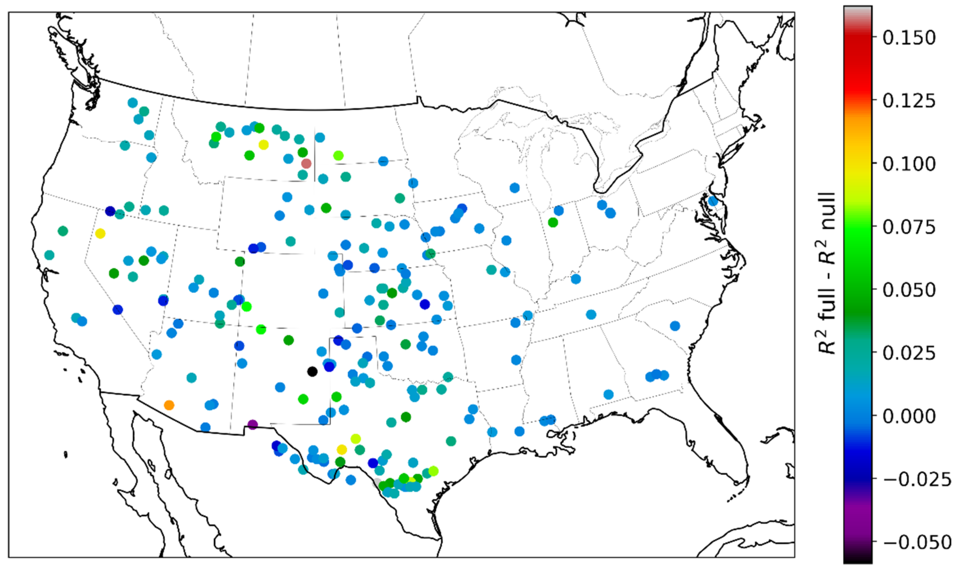
4.4. LAI Estimations
5. Discussion
5.1. Theoretical Additive Information of L-Band VOD and SM
5.2. Additive Information of L-Band SM and VOD for LAI Anomaly
5.3. Additive Information of SM and VOD for LAI
5.4. Uncertainties, Limitations and Potential Applications
6. Conclusions
Supplementary Materials
Author Contributions
Funding
Institutional Review Board Statement
Informed Consent Statement
Data Availability Statement
Acknowledgments
Conflicts of Interest
References
- Way, D.A.; Montgomery, R.A. Photoperiod constraints on tree phenology, performance and migration in a warming world. Plant Cell Environ. 2014, 38, 1725–1736. [Google Scholar] [CrossRef]
- Gornall, J.; Betts, R.; Burke, E.; Clark, R.; Camp, J.; Willett, K.; Wiltshire, A. Implications of climate change for agricultural productivity in the early twenty-first century. Philos. Trans. R. Soc. B Biol. Sci. 2010, 365, 2973–2989. [Google Scholar] [CrossRef]
- Piao, S.; Fang, J.; Zhou, L.; Ciais, P.; Zhu, B. Variations in satellite-derived phenology in China’s temperate vegetation. Glob. Chang. Biol. 2006, 12, 672–685. [Google Scholar] [CrossRef]
- Justice, C.; Townshend, J.R.G.; Holben, B.N.; Tucker, C.J. Analysis of the phenology of global vegetation using meteorological satellite data. Int. J. Remote Sens. 1985, 6, 1271–1318. [Google Scholar] [CrossRef]
- Piao, S.; Liu, Q.; Chen, A.; Janssens, I.A.; Fu, Y.; Dai, J.; Liu, L.; Lian, X.; Shen, M.; Zhu, X. Plant phenology and global climate change: Current progresses and challenges. Glob. Chang. Biol. 2019, 25, 1922–1940. [Google Scholar] [CrossRef]
- Liu, Q.; Piao, S.; Janssens, I.A.; Fu, Y.; Peng, S.; Lian, X.; Ciais, P.; Myneni, R.B.; Peñuelas, J.; Wang, T. Extension of the growing season increases vegetation exposure to frost. Nat. Commun. 2018, 9, 426. [Google Scholar] [CrossRef] [PubMed] [Green Version]
- Gerard, F.F.; George, C.T.; Hayman, G.; Chavana-Bryant, C.; Weedon, G.P. Leaf phenology amplitude derived from MODIS NDVI and EVI: Maps of leaf phenology synchrony for Meso- and South America. Geosci. Data J. 2020, 7, 13–26. [Google Scholar] [CrossRef] [Green Version]
- Delbart, N.; Kergoat, L.; Le Toan, T.; Lhermitte, J.; Picard, G. Determination of phenological dates in boreal regions using normalized difference water index. Remote Sens. Environ. 2005, 97, 26–38. [Google Scholar] [CrossRef] [Green Version]
- Gao, L.; Wang, X.; Johnson, B.A.; Tian, Q.; Wang, Y.; Verrelst, J.; Mu, X.; Gu, X. Remote sensing algorithms for estimation of fractional vegetation cover using pure vegetation index values: A review. ISPRS J. Photogramm. Remote Sens. 2020, 159, 364–377. [Google Scholar] [CrossRef]
- Ju, J.; Masek, J.G. The vegetation greenness trend in Canada and US Alaska from 1984–2012 Landsat data. Remote Sens. Environ. 2016, 176, 1–16. [Google Scholar] [CrossRef]
- Xue, J.; Su, B. Significant Remote Sensing Vegetation Indices: A Review of Developments and Applications. J. Sens. 2017, 2017, 1–17. [Google Scholar] [CrossRef] [Green Version]
- Chen, M.; Willgoose, G.R.; Saco, P.M. Investigating the impact of leaf area index temporal variability on soil moisture predictions using remote sensing vegetation data. J. Hydrol. 2015, 522, 274–284. [Google Scholar] [CrossRef]
- Martinez, B.; Cassiraga, E.; Camacho, F.; Garcia-Haro, J. Geostatistics for Mapping Leaf Area Index over a Cropland Landscape: Efficiency Sampling Assessment. Remote Sens. 2010, 2, 2584–2606. [Google Scholar] [CrossRef] [Green Version]
- Sun, L.; Gao, F.; Anderson, M.C.; Kustas, W.P.; Alsina, M.M.; Sanchez, L.; Sams, B.; McKee, L.; Dulaney, W.; White, W.A.; et al. Daily Mapping of 30 m LAI and NDVI for Grape Yield Prediction in California Vineyards. Remote Sens. 2017, 9, 317. [Google Scholar] [CrossRef] [Green Version]
- Li, Z.; Wang, J.; Tang, H.; Huang, C.; Yang, F.; Chen, B.; Wang, X.; Xin, X.; Ge, Y. Predicting Grassland Leaf Area Index in the Meadow Steppes of Northern China: A Comparative Study of Regression Approaches and Hybrid Geostatistical Methods. Remote Sens. 2016, 8, 632. [Google Scholar] [CrossRef] [Green Version]
- Darvishzadeh, R.; Skidmore, A.; Schlerf, M.; Atzberger, C.; Corsi, F.; Cho, M. LAI and chlorophyll estimation for a heterogeneous grassland using hyperspectral measurements. ISPRS J. Photogramm. Remote Sens. 2008, 63, 409–426. [Google Scholar] [CrossRef]
- Xie, Q.; Huang, W.; Liang, D.; Chen, P.; Wu, C.; Yang, G.; Zhang, J.; Huang, L.; Zhang, D. Leaf Area Index Estimation Using Vegetation Indices Derived from Airborne Hyperspectral Images in Winter Wheat. IEEE J. Sel. Top. Appl. Earth Obs. Remote Sens. 2014, 7, 3586–3594. [Google Scholar] [CrossRef]
- Houborg, R.; Boegh, E. Mapping leaf chlorophyll and leaf area index using inverse and forward canopy reflectance modeling and SPOT reflectance data. Remote Sens. Environ. 2008, 112, 186–202. [Google Scholar] [CrossRef]
- Omer, G.; Mutanga, O.; Abdel-Rahman, E.M.; Adam, E. Empirical Prediction of Leaf Area Index (LAI) of Endangered Tree Species in Intact and Fragmented Indigenous Forests Ecosystems Using WorldView-2 Data and Two Robust Machine Learning Algorithms. Remote Sens. 2016, 8, 324. [Google Scholar] [CrossRef] [Green Version]
- Houborg, R.; McCabe, M.F. A hybrid training approach for leaf area index estimation via Cubist and random forests machine-learning. ISPRS J. Photogramm. Remote Sens. 2018, 135, 173–188. [Google Scholar] [CrossRef]
- Qu, Y.; Zhuang, Q. Modeling leaf area index in North America using a process-based terrestrial ecosystem model. Ecosphere 2018, 9, e02046. [Google Scholar] [CrossRef] [Green Version]
- Wigneron, J.-P.; Li, X.; Frappart, F.; Fan, L.; Al-Yaari, A.; De Lannoy, G.; Liu, X.; Wang, M.; Le Masson, E.; Moisy, C. SMOS-IC data record of soil moisture and L-VOD: Historical development, applications and perspectives. Remote Sens. Environ. 2021, 254, 112238. [Google Scholar] [CrossRef]
- Grant, J.; Wigneron, J.-P.; De Jeu, R.; Lawrence, H.; Mialon, A.; Richaume, P.; Al Bitar, A.; Drusch, M.; van Marle, M.; Kerr, Y. Comparison of SMOS and AMSR-E vegetation optical depth to four MODIS-based vegetation indices. Remote Sens. Environ. 2016, 172, 87–100. [Google Scholar] [CrossRef]
- Tian, F.; Wigneron, J.-P.; Ciais, P.; Chave, J.; Ogée, J.; Peñuelas, J.; Ræbild, A.; Domec, J.-C.; Tong, X.; Brandt, M.; et al. Coupling of ecosystem-scale plant water storage and leaf phenology observed by satellite. Nat. Ecol. Evol. 2018, 2, 1428–1435. [Google Scholar] [CrossRef] [Green Version]
- Lawrence, H.; Wigneron, J.-P.; Richaume, P.; Novello, N.; Grant, J.; Mialon, A.; Al Bitar, A.; Merlin, O.; Guyon, D.; Leroux, D.; et al. Comparison between SMOS Vegetation Optical Depth products and MODIS vegetation indices over crop zones of the USA. Remote Sens. Environ. 2014, 140, 396–406. [Google Scholar] [CrossRef]
- Momen, M.; Wood, J.D.; Novick, K.A.; Pangle, R.; Pockman, W.T.; McDowell, N.G.; Konings, A.G. Interacting Effects of Leaf Water Potential and Biomass on Vegetation Optical Depth. J. Geophys. Res. Biogeosci. 2017, 122, 3031–3046. [Google Scholar] [CrossRef]
- Wang, C.; Fu, B.; Zhang, L.; Xu, Z. Soil moisture–plant interactions: An ecohydrological review. J. Soils Sediments 2018, 19, 1–9. [Google Scholar] [CrossRef]
- Bassiouni, M.; Good, S.P.; Still, C.J.; Higgins, C.W. Plant Water Uptake Thresholds Inferred from Satellite Soil Moisture. Geophys. Res. Lett. 2020, 47, 47. [Google Scholar] [CrossRef] [Green Version]
- Boke-Olén, N.; Ardö, J.; Eklundh, L.; Holst, T.; Lehsten, V. Remotely sensed soil moisture to estimate savannah NDVI. PLoS ONE 2018, 13, e0200328. [Google Scholar] [CrossRef]
- Tong, C.; Wang, H.; Magagi, R.; Goïta, K.; Zhu, L.; Yang, M.; Deng, J. Soil Moisture Retrievals by Combining Passive Microwave and Optical Data. Remote Sens. 2020, 12, 3173. [Google Scholar] [CrossRef]
- Entekhabi, D.; Njoku, E.G.; O’Neill, P.E.; Kellogg, K.H.; Crow, W.T.; Edelstein, W.N.; Entin, J.K.; Goodman, S.D.; Jackson, T.J.; Johnson, J.; et al. The Soil Moisture Active Passive (SMAP) Mission. Proc. IEEE 2010, 98, 704–716. [Google Scholar] [CrossRef]
- Colliander, A.; Cosh, M.H.; Misra, S.; Jackson, T.J.; Crow, W.T.; Chan, S.; Bindlish, R.; Chae, C.; Collins, C.H.; Yueh, S.H. Validation and scaling of soil moisture in a semi-arid environment: SMAP validation experiment 2015 (SMAPVEX15). Remote Sens. Environ. 2017, 196, 101–112. [Google Scholar] [CrossRef]
- Chan, S.K.; Bindlish, R.; O’Neill, P.E.; Njoku, E.; Jackson, T.; Colliander, A.; Chen, F.; Burgin, M.; Dunbar, S.; Piepmeier, J.; et al. Assessment of the SMAP Passive Soil Moisture Product. IEEE Trans. Geosci. Remote Sens. 2016, 54, 4994–5007. [Google Scholar] [CrossRef]
- Burgin, M.S.; Colliander, A.; Njoku, E.G.; Chan, S.K.; Cabot, F.; Kerr, Y.H.; Bindlish, R.; Jackson, T.J.; Entekhabi, D.; Yueh, S.H. A Comparative Study of the SMAP Passive Soil Moisture Product with Existing Satellite-Based Soil Moisture Products. IEEE Trans. Geosci. Remote Sens. 2017, 55, 2959–2971. [Google Scholar] [CrossRef] [PubMed]
- Colliander, A.; Jackson, T.J.; Bindlish, R.; Chan, S.; Das, N.; Kim, S.B.; Cosh, M.H.; Dunbar, R.S.; Dang, L.; Pashaian, L.; et al. Validation of SMAP surface soil moisture products with core validation sites. Remote Sens. Environ. 2017, 191, 215–231. [Google Scholar] [CrossRef]
- Tian, F.; Brandt, M.; Liu, Y.Y.; Verger, A.; Tagesson, T.; Diouf, A.A.; Rasmussen, K.; Mbow, C.; Wang, Y.; Fensholt, R. Remote sensing of vegetation dynamics in drylands: Evaluating vegetation optical depth (VOD) using AVHRR NDVI and in situ green biomass data over West African Sahel. Remote Sens. Environ. 2016, 177, 265–276. [Google Scholar] [CrossRef] [Green Version]
- Feldman, A.F.; Gianotti, D.J.S.; Konings, A.G.; McColl, K.A.; Akbar, R.; Salvucci, G.D.; Entekhabi, D. Moisture pulse-reserve in the soil-plant continuum observed across biomes. Nat. Plants 2018, 4, 1026–1033. [Google Scholar] [CrossRef]
- Global Subsets Tool: MODIS/VIIRS Land Products. Available online: https://modis.ornl.gov/globalsubset/ (accessed on 24 February 2020).
- Vannan, S.K.S.; Cook, R.B.; Holladay, S.K.; Olsen, L.M.; Dadi, U.; Wilson, B.E. A Web-Based Subsetting Service for Regional Scale MODIS Land Products. IEEE J. Sel. Top. Appl. Earth Obs. Remote Sens. 2009, 2, 319–328. [Google Scholar] [CrossRef]
- Fang, H.; Wei, S.; Liang, S. Validation of MODIS and CYCLOPES LAI products using global field measurement data. Remote Sens. Environ. 2012, 119, 43–54. [Google Scholar] [CrossRef]
- Yan, K.; Park, T.; Yan, G.; Liu, Z.; Yang, B.; Chen, C.; Nemani, R.R.; Knyazikhin, Y.; Myneni, R.B. Evaluation of MODIS LAI/FPAR Product Collection 6. Part 2: Validation and Intercomparison. Remote Sens. 2016, 8, 460. [Google Scholar] [CrossRef] [Green Version]
- Kandasamy, S.; Baret, F.; Verger, A.; Neveux, P.; Weiss, M. A comparison of methods for smoothing and gap filling time series of remote sensing observations—Application to MODIS LAI products. Biogeosciences 2013, 10, 4055–4071. [Google Scholar] [CrossRef] [Green Version]
- Sulla-Menashe, D.; Gray, J.M.; Abercrombie, S.P.; Friedl, M.A. Hierarchical mapping of annual global land cover 2001 to present: The MODIS Collection 6 Land Cover product. Remote Sens. Environ. 2019, 222, 183–194. [Google Scholar] [CrossRef]
- Kwa, C. Local Ecologies and Global Science. Soc. Stud. Sci. 2005, 35, 923–950. [Google Scholar] [CrossRef]
- Reichle, R.; De Lannoy, G.; Koster, R.D.; Crow, W.T.; Kimball, J.S.; Liu, Q. SMAP L4 Global 3-Hourly 9 km EASE-Grid Surface and Root Zone Soil Moisture Geophysical Data, Version 4; NASA National Snow and Ice Data Center Distributed Active Archive Center: Boulder, CO, USA, 2018. [CrossRef]
- National Snow & Ice Data Center NASA Distributed Active Archive Center (DACC) at NSIDC. Available online: https://nsidc.org/data/smap/smap-data.html (accessed on 2 October 2019).
- Scranton, K.; Amarasekare, P. Predicting phenological shifts in a changing climate. Proc. Natl. Acad. Sci. USA 2017, 114, 13212–13217. [Google Scholar] [CrossRef] [Green Version]
- Bradley, A.V.; Gerard, F.F.; Barbier, N.; Weedon, G.P.; Anderson, L.O.; Huntingford, C.; Aragão, L.E.O.C.; Zelazowski, P.; Arai, E. Relationships between phenology, radiation and precipitation in the Amazon region. Glob. Chang. Biol. 2011, 17, 2245–2260. [Google Scholar] [CrossRef]
- O’Neill, P.E.; Chan, S.; Njoku, E.G.; Jackson, T.; Bindlish, R. SMAP Enhanced L2 Radiometer Global Daily 9 km EASE-Grid Soil Moisture, Version 3; NASA National Snow and Ice Data Center Distributed Active Archive Center: Boulder, CO, USA, 2019. [CrossRef]
- Chaubell, M.J.; Yueh, S.H.; Dunbar, R.S.; Colliander, A.; Chen, F.; Chan, S.K.; Entekhabi, D.; Bindlish, R.; O’Neill, P.E.; Asanuma, J.; et al. Improved SMAP Dual-Channel Algorithm for the Retrieval of Soil Moisture. IEEE Trans. Geosci. Remote Sens. 2020, 58, 3894–3905. [Google Scholar] [CrossRef]
- Wigneron, J.-P.; Jackson, T.; O’Neill, P.; De Lannoy, G.; de Rosnay, P.; Walker, J.; Ferrazzoli, P.; Mironov, V.; Bircher, S.; Grant, J.; et al. Modelling the passive microwave signature from land surfaces: A review of recent results and application to the L-band SMOS & SMAP soil moisture retrieval algorithms. Remote Sens. Environ. 2017, 192, 238–262. [Google Scholar] [CrossRef]
- Kraskov, A.; Stögbauer, H.; Grassberger, P. Estimating mutual information. Remote Sens. Environ. 2004, 69, 066138. [Google Scholar] [CrossRef] [Green Version]
- Scott, D.W. Scott’s rule. Wiley Interdiscip. Rev. Comput. Stat. 2010, 2, 497–502. [Google Scholar] [CrossRef]
- Zhang, Z.; Grabchak, M. Bias Adjustment for a Nonparametric Entropy Estimator. Entropy 2013, 15, 1999–2011. [Google Scholar] [CrossRef]
- Breiman, L. Random forests. Mach. Learn. 2001, 45, 5–32. [Google Scholar] [CrossRef] [Green Version]
- Probst, P.; Wright, M.N.; Boulesteix, A. Hyperparameters and tuning strategies for random forest. Wiley Interdiscip. Rev. Data Min. Knowl. Discov. 2019, 9, 9. [Google Scholar] [CrossRef] [Green Version]
- Hohenegger, C.; Brockhaus, P.; Bretherton, C.S.; Schär, C. The Soil Moisture–Precipitation Feedback in Simulations with Explicit and Parameterized Convection. J. Clim. 2009, 22, 5003–5020. [Google Scholar] [CrossRef]
- Asharaf, S.; Dobler, A.; Ahrens, B. Soil Moisture–Precipitation Feedback Processes in the Indian Summer Monsoon Season. J. Hydrometeorol. 2012, 13, 1461–1474. [Google Scholar] [CrossRef]
- Hsu, H.; Lo, M.-H.; Guillod, B.P.; Miralles, D.G.; Kumar, S. Relation between precipitation location and antecedent/subsequent soil moisture spatial patterns. J. Geophys. Res. Atmos. 2017, 122, 6319–6328. [Google Scholar] [CrossRef]
- Vittucci, C.; Laurin, G.V.; Tramontana, G.; Ferrazzoli, P.; Guerriero, L.; Papale, D. Vegetation optical depth at L-band and above ground biomass in the tropical range: Evaluating their relationships at continental and regional scales. Int. J. Appl. Earth Obs. Geoinf. 2019, 77, 151–161. [Google Scholar] [CrossRef]
- Liu, R.; Wen, J.; Wang, X.; Wang, Z.; Li, Z.; Xie, Y.; Zhu, L.; Li, D. Derivation of Vegetation Optical Depth and Water Content in the Source Region of the Yellow River using the FY-3B Microwave Data. Remote Sens. 2019, 11, 1536. [Google Scholar] [CrossRef] [Green Version]
- Zhang, R.; Kim, S.; Sharma, A. A comprehensive validation of the SMAP Enhanced Level-3 Soil Moisture product using ground measurements over varied climates and landscapes. Remote Sens. Environ. 2019, 223, 82–94. [Google Scholar] [CrossRef]
- Chan, S.; Bindlish, R.; O’Neill, P.; Jackson, T.; Njoku, E.; Dunbar, S.; Chaubell, J.; Piepmeier, J.; Yueh, S.; Entekhabi, D.; et al. Development and assessment of the SMAP enhanced passive soil moisture product. Remote Sens. Environ. 2018, 204, 931–941. [Google Scholar] [CrossRef] [PubMed] [Green Version]
- El Hajj, M.; Baghdadi, N.; Bazzi, H.; Zribi, M. Penetration Analysis of SAR Signals in the C and L Bands for Wheat, Maize, and Grasslands. Remote Sens. 2018, 11, 31. [Google Scholar] [CrossRef] [Green Version]
- Escorihuela, M.; Chanzy, A.; Wigneron, J.; Kerr, Y. Effective soil moisture sampling depth of L-band radiometry: A case study. Remote Sens. Environ. 2010, 114, 995–1001. [Google Scholar] [CrossRef] [Green Version]
- Stavi, I. Wildfires in Grasslands and Shrublands: A Review of Impacts on Vegetation, Soil, Hydrology, and Geomorphology. Water 2019, 11, 1042. [Google Scholar] [CrossRef] [Green Version]
- Bonan, L.; Good, S.P. Information–based uncertainty decomposition in dual channel microwave remote sensing of soil moisture. Hydrol. Earth Syst. Sci. Discuss. 2020, 534, 1–16. [Google Scholar] [CrossRef]
- Cowling, S.A.; Field, C.B. Environmental control of leaf area production: Implications for vegetation and land-surface modeling. Glob. Biogeochem. Cycles 2003, 17, 7-1. [Google Scholar] [CrossRef]
- Roosjen, P.P.; Brede, B.; Suomalainen, J.M.; Bartholomeus, H.M.; Kooistra, L.; Clevers, J.G. Improved estimation of leaf area index and leaf chlorophyll content of a potato crop using multi-angle spectral data—Potential of unmanned aerial vehicle imagery. Int. J. Appl. Earth Obs. Geoinf. 2018, 66, 14–26. [Google Scholar] [CrossRef]
- Korhonen, L.; Hadi; Packalen, P.; Rautiainen, M. Comparison of Sentinel-2 and Landsat 8 in the estimation of boreal forest canopy cover and leaf area index. Remote Sens. Environ. 2017, 195, 259–274. [Google Scholar] [CrossRef]
- Li, S.; Yuan, F.; Ata-Ui-Karim, S.T.; Zheng, H.; Cheng, T.; Liu, X.; Tian, Y.; Zhu, Y.; Cao, W.; Cao, Q. Combining Color Indices and Textures of UAV-Based Digital Imagery for Rice LAI Estimation. Remote Sens. 2019, 11, 1763. [Google Scholar] [CrossRef] [Green Version]
- Li, R.; Li, C.-J.; Dong, Y.-Y.; Liu, F.; Wang, J.-H.; Yang, X.-D.; Pan, Y.-C. Assimilation of Remote Sensing and Crop Model for LAI Estimation Based on Ensemble Kaiman Filter. Agric. Sci. China 2011, 10, 1595–1602. [Google Scholar] [CrossRef]
- Dube, T.; Pandit, S.; Shoko, C.; Ramoelo, A.; Mazvimavi, D.; Dalu, T. Numerical Assessments of Leaf Area Index in Tropical Savanna Rangelands, South Africa Using Landsat 8 OLI Derived Metrics and In-Situ Measurements. Remote Sens. 2019, 11, 829. [Google Scholar] [CrossRef] [Green Version]
- Gonsamo, A.; Chen, J.M. Improved LAI Algorithm Implementation to MODIS Data by Incorporating Background, Topography, and Foliage Clumping Information. IEEE Trans. Geosci. Remote Sens. 2013, 52, 1076–1088. [Google Scholar] [CrossRef]


| full Model R2s | null Model R2s | full Model R2s–null Model R2s | Percentage Improvements | Number of Sites | |
|---|---|---|---|---|---|
| Mean | Mean | Mean | (% of null) | n | |
| Grasslands | 0.24 ** | 0.16 ** | 0.08 ** | 50% | 120 |
| Shrublands | 0.17 ** | 0.14 ** | 0.03 ** | 19% | 27 |
| Croplands | 0.23 ** | 0.15 ** | 0.08 ** | 56% | 47 |
| Savannas | 0.20 ** | 0.12 ** | 0.08 ** | 57% | 22 |
| All | 0.22 ** | 0.15 ** | 0.07 ** | 50% | 216 |
| full Model ubRMSE | null Model ubRMSE | null Model ubRMSE– full Model ubRMSE | Percentage Improvements | Number of Sites | |
|---|---|---|---|---|---|
| Mean | Mean | Mean | (% of null) | n | |
| Grasslands | 0.118 ** | 0.126 ** | 0.008 ** | 5.7% | 120 |
| Shrublands | 0.053 ** | 0.054 ** | 0.001 * | 1.7% | 27 |
| Croplands | 0.193 ** | 0.203 ** | 0.01 ** | 5.1% | 47 |
| Savannas | 0.157 ** | 0.165 ** | 0.008 ** | 4.4% | 22 |
| All | 0.130 ** | 0.137 ** | 0.007 ** | 5.2% | 216 |
| full Model R2s | null Model R2s | Climatology R2s | full Model R2s–null Model R2s | Percentage Improvements | Number of Sites | |
|---|---|---|---|---|---|---|
| Mean | Mean | Mean | Mean | (% of null) | n | |
| Grasslands | 0.82 ** | 0.80 ** | 0.73 ** | 0.02 ** | 2.7% | 120 |
| Shrublands | 0.64 ** | 0.63 ** | 0.50 ** | 0.01 * | 2.3% | 27 |
| Croplands | 0.92 ** | 0.91 ** | 0.89 ** | 0.01 ** | 1.1% | 47 |
| Savannas | 0.91 ** | 0.90 ** | 0.86 ** | 0.01 ** | 1.0% | 22 |
| All | 0.83 ** | 0.81 ** | 0.75 ** | 0.02 ** | 2.1% | 216 |
Publisher’s Note: MDPI stays neutral with regard to jurisdictional claims in published maps and institutional affiliations. |
© 2021 by the authors. Licensee MDPI, Basel, Switzerland. This article is an open access article distributed under the terms and conditions of the Creative Commons Attribution (CC BY) license (https://creativecommons.org/licenses/by/4.0/).
Share and Cite
Li, B.; Good, S.P.; URycki, D.R. The Value of L-Band Soil Moisture and Vegetation Optical Depth Estimates in the Prediction of Vegetation Phenology. Remote Sens. 2021, 13, 1343. https://doi.org/10.3390/rs13071343
Li B, Good SP, URycki DR. The Value of L-Band Soil Moisture and Vegetation Optical Depth Estimates in the Prediction of Vegetation Phenology. Remote Sensing. 2021; 13(7):1343. https://doi.org/10.3390/rs13071343
Chicago/Turabian StyleLi, Bonan, Stephen P. Good, and Dawn R. URycki. 2021. "The Value of L-Band Soil Moisture and Vegetation Optical Depth Estimates in the Prediction of Vegetation Phenology" Remote Sensing 13, no. 7: 1343. https://doi.org/10.3390/rs13071343