Unified Low-Rank Subspace Clustering with Dynamic Hypergraph for Hyperspectral Image

Abstract

Low-rank representation with hypergraph regularization has achieved great success in hyperspectral imagery, which can explore global structure, and further incorporate local information. Existing hypergraph learning methods only construct the hypergraph by a fixed similarity matrix or are adaptively optimal in original feature space; they do not update the hypergraph in subspace-dimensionality. In addition, the clustering performance obtained by the existing k-means-based clustering methods is unstable as the k-means method is sensitive to the initialization of the cluster centers. In order to address these issues, we propose a novel unified low-rank subspace clustering method with dynamic hypergraph for hyperspectral images (HSIs). In our method, the hypergraph is adaptively learned from the low-rank subspace feature, which can capture a more complex manifold structure effectively. In addition, we introduce a rotation matrix to simultaneously learn continuous and discrete clustering labels without any relaxing information loss. The unified model jointly learns the hypergraph and the discrete clustering labels, in which the subspace feature is adaptively learned by considering the optimal dynamic hypergraph with the self-taught property. The experimental results on real HSIs show that the proposed methods can achieve better performance compared to eight state-of-the-art clustering methods.

1. Introduction

Hyperspectral image (HSI) classification is an important problem in the remote sensing community. Extensive prior literature addresses the classification in the framework of supervised classification [1,2,3], in which the training of the classifier relies on the labeled data (with ground-truth information). However, the labeled datasets are strained and impossible to obtain in some applications by human capacity [4]. With the aim of exploiting the unlabeled remote sensing data, unsupervised classification methods containing the segmentation of the dataset into several groups with no prior label information are necessary.

According to the existing literature, clustering methods are divided into several categories [5]. The two most popular categories suitable for the characteristics of the HSIs are centroid-based methods and spectral-based methods. Among the centroid-based clustering methods, k-means [6] and fuzzy c-means (FCM) [7] get more attention due to their computational efficiency and simplicity, which group pixels by finding the minimum distance between pixels and each clustering centroid through iterative update. Recently, the spectral-based clustering methods have been highly popular and have been widely used for hyperspectral data clustering. In general, these methods construct a similarity matrix based on the original data first, then apply the centroid-based methods to the eigenspaces of the Laplacian matrix to segment pixels. Specifically, the locally spectral clustering (LSC) [8] and the globally spectral clustering (GSC) [9] use the local and global neighbors about each pixel to construct the similarity matrix which represents the relationship between pairs of pixels respectively, and applies k-means on the eigenspace of the Laplacian matrices, but they cannot distinguish between subspaces the pixels should belong to. Otherwise, the large spectral variability results in the uniform feature point distribution, which increased the difficulty of HSI clustering [5]. The recently developed sparse subspace clustering (SSC) [10,11] and low-rank subspace clustering (LRSC) [12,13] methods use the sparse and low-rank representation coefficients to define the adjacent matrix, and apply spectral clustering to obtain the segmentation result. However, compared with SSC, LRSC is better at exploring the global structure information by finding the lowest-rank representation of all the data jointly. Nevertheless, the original LRSC model cannot explore the local latent structure information of the data while exploiting the corresponding subspaces.

Inspired by the theory of manifold learning in image processing [14], Lu et al. [15] proposed the graph-embedded low-rank representation (GLRR) by incorporating graph regularization into low-rank representation objective function. However, the general graph regularization model only uses the paired relationship between two pixels, which cannot excavate the complex high-order relationships of the pixels. In fact, the relationship between the hyperspectral pixels we are interested in is not just a pairwise relationship between two pixels, but a plural or even more complex relationship. Instead of considering pairwise relations, the hypergraph models the data manifold structures by exploring the high-order relations among data points, which is first proposed by Berge [16]. Zhou et al. [17] combined the powerful methodology of spectral clustering to extend originally undirected graph to hypergraph. Then, hypergraph is widely used in feature extraction [18], band selection [19], dimension reduction [20], and noise reduction [21] in hyperspectral images. According to the extensive prior literature, the methods associated with hypergraph based on representation learning are divided into two categories. One is using the representation coefficient as the hyperedge weight to construct hypergraph, such as [2,22] regards sparse and low-rank coefficients as a new feature to measure the similarity of the pixels and adaptively select neighbors for constructing the hypergraph, respectively. The other is using hypergraph as regularization to optimal representation coefficient by capturing intrinsic geometrical structure. Gao et al. [23] first introduced hypergraph into sparse coding, in which hypergraph explores the similarity information among the pixels within the same hyperedge, and simultaneously updates the sparse representation coefficient of them to be similar to each other. Motivated by the idea of hypergraph regularization, it was introduced into non-negative matrix factorization [24], sparse NMF [25], low-rank representation [26,27].

It is noteworthy that there are two main problems in existing hypergraph-based representation learning methods. First, the pre-constructed hypergraph is usually learned from the original data with a certain distance measurement but not optimized dynamically. Then, Zhang et al. [28] proposed a unified framework for data structure estimation and feature selection, which update the hypergraph weight in the hypergraph learning process. In Reference [29], a dynamic hypergraph structure learning method was proposed, in which the incidence matrix of hypergraph can be learned by considering the data correlation on both the label space and the feature space. In addition, the data from the original feature space may contain various of noises, which could degenerate the performance since these methods highly depend on the constructed hypergraph. Zhu et al. [30,31] proposed an unsupervised sparse feature selection method by embedding a hypergraph Laplacian regularizer, in which the hypergraph was learned dynamically from the optimized sparse subspace feature. Otherwise, the hypergraph was adaptively learned from the latent representation space, which can robustly characterize the intrinsic data structure [32,33]. Second, the clustering performance obtained by the existing k-means-based methods is unstable as the initialization of the cluster centers has too much impact on the performance of the k-means method. Therefore, it is necessary to construct a unified framework and directly generate discrete clustering labels [34,35,36]. However, the existing unified clustering framework is based on the general graph structure, which may lead to significant information loss and reduce the performance of the clustering algorithm.

To address the issues, we propose a novel unified dynamic hypergraph low-rank subspace clustering method for hyperspectral images, known as UDHLR. First, we develop a dynamic hypergraph low-rank subspace clustering method, known as DHLR, where the hypergraph regularization is used to preserve the local complex structure of the low-dimensional data. Meanwhile, the hypergraph is adaptively learned from the low-rank subspace feature. However, the DHLR algorithm works in two separate steps: learning the low-rank coefficient matrix as similarity graph; generating the discrete clustering label by the k-means method. Therefore, we integrate these two subtasks into a unified framework, in which low-rank representation coefficient, hypergraph structure and discrete clustering label are optimized by using the results of the others to get an overall optimal result. The main contributions of our methods are summarized as follows:

(1)

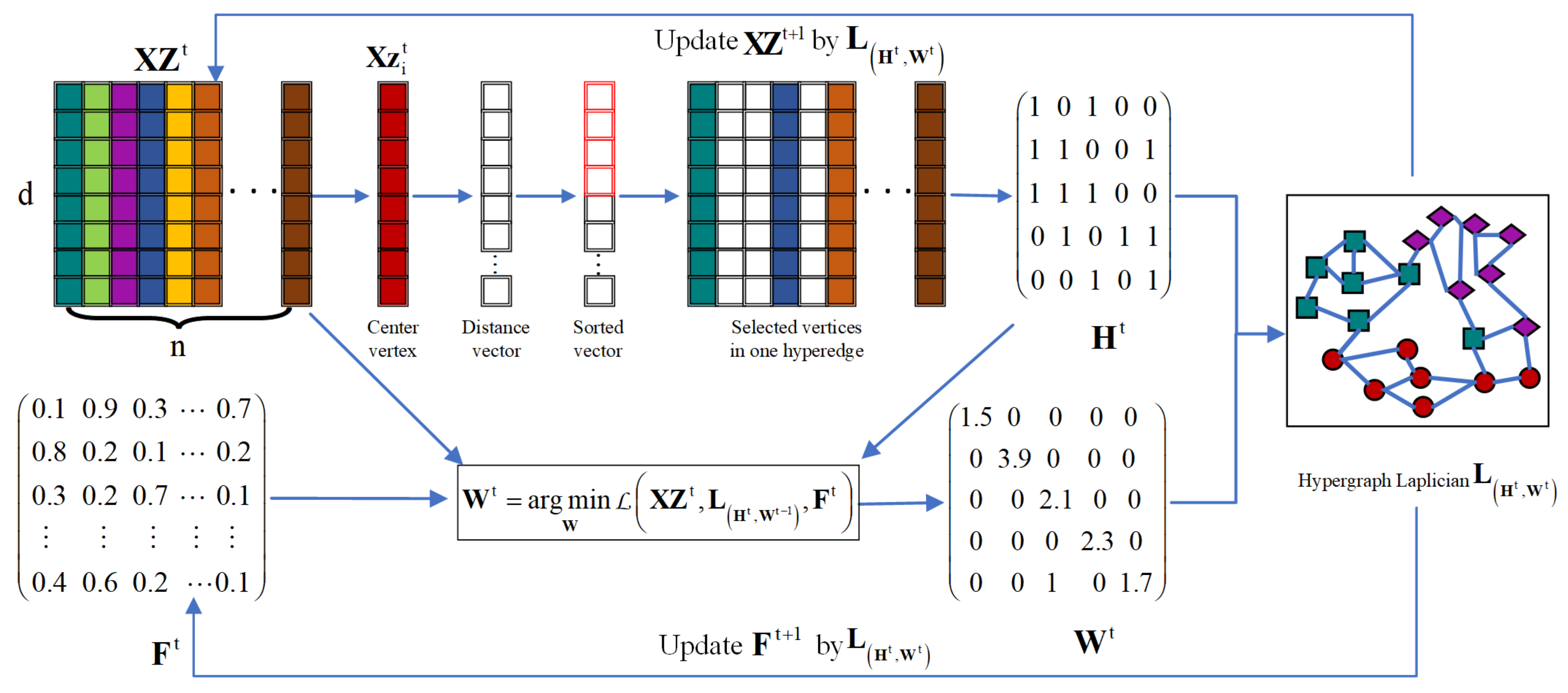
Instead of pre-constructing a fixed hypergraph incidence and weight matrices, the hypergraph is adaptively learned from the low-rank subspace feature. The dynamically constructed hypergraph is well structured and theoretically suitable for clustering.

(2)

The proposed method simultaneously optimizes continuous labels, and discrete cluster labels by a rotation matrix without any relaxing information loss.

(3)

It jointly learns the similarity hypergraph from the learned low-rank subspace data and the discrete clustering labels by solving a unified optimization problem, in which the low-rank subspace feature and hypergraph are adaptively learned by considering the clustering performance and the continuous clustering labels just serve as intermediate products.

The remainder of this paper is organized as follows: Section 2 revisits the low-rank representation and hypergraph. Section 3 describes the proposed DHLR and UDHLR models. Section 4 presents the experimental setting and experimental results. Section 5 presents the discussions about computation complexity. Finally, concludes are presented in Section 6. The framework of the proposed methods is shown in Figure 1.

2. Related Work

The important notations in the paper are summarized in

Table 1. Important notation used in this paper.

Notation	Definition
d	Number of bands
n	Number of pixels
c	Number of the classes
X	Hyperspectral image
Z	Low-rank representation matrix
N	Noise matrix
G	A hypergraph
V	The vertexes of hypergraph
E	The hyperedges of hypergraph
W	The weight of hyperedges
H	The incidence matrix of hypergraph
L	Hypergraph Laplacian matrix
Q	Rotation matrix
F	The continuous label indicator matrix
Y	The label matrix
t	Number of iterations

.

2.1. Low-Rank Representation

Let $\mathbf{X}=\left[{\mathbf{x}}_1,{\mathbf{x}}_2,\dots ,{\mathbf{x}}_n\right] \in R^{d\times n}$ denotes a hyperspectral image with n samples, ${\mathbf{x}}_i\in R^d$ represents the i-th pixel with d spectral bands. Low-rank representation (LRR) attempts to solve the following objective function to seek the lowest-rank representation for clustering

$$\underset{\mathbf{Z}}{\min }\mathrm{rank}\left(\mathbf{Z}\right)\mathrm{s}.\mathrm{t}.\mathbf{X}=\mathbf{XZ}+\mathbf{N},$$

(1)

where $\mathbf{Z}\in R^{n\times n}$ denotes the lowest-rank representation matrix under a self-expressive dictionary [13], $\mathrm{rank}\left(\mathbf{Z}\right)$ is the rank of matrix Z, N is a sparse matrix of outliers. However, the rank minimization problem is NP-hard and difficult to optimize, thus the nuclear norm is adopted to address this issue, yielding the following optimization [13]:

$$\underset{\mathbf{Z}}{\min }{∥\mathbf{Z}∥}_{*}\mathrm{s}.\mathrm{t}.\mathbf{X}=\mathbf{XZ}+\mathbf{N},$$

(2)

where ${∥\mathbf{Z}∥}_{*}$ is the nuclear norm constraint of matrix Z and is calculated as ${∥\mathbf{Z}∥}_{*}=\sum _i^n{\delta }_i$, ${\delta }_i$ is the i-th singular value of matrix Z. The representation matrix Z can be solved by optimizing the above problem via the inexact augmented Lagrange multiplier (ALM) method [37]. Finally, the adjacency matrix $\left|\mathbf{Z}\right| + {\left|\mathbf{Z}\right|}^{\mathrm{T}}$ as the edge weights can be constructed with the obtained low-rank coefficient matrix, and the clustering result is obtained by applying the k-means to the eigenspaces of the Laplacian matrix induced by the adjacency matrix.

2.2. Hypergraph

The relationship between pixels we are interested in is not just a pairwise relationship between two pixels, but a plural or even more complex relationship. When simply compress the multivariate relationship into a pairwise relationship between two pixels, it would inevitably lose a lot of useful information, thus it would affect the accuracy of feature learning to a certain extent [19].

Let $\mathbf{G}=\left(\mathbf{V},\mathbf{E},\mathbf{W}\right)$ denote a hypergraph, where $\mathbf{V}={\left[{\mathbf{v}}_i\right]}_{i=1}^n$ and $\mathbf{E}={\left[{\mathbf{e}}_i\right]}_{i=1}^n$ are the set of vertexes and hyperedges, respectively. The dataset $\mathbf{X}$ can be used to make up the set of the vertexes $\mathbf{V}$. $\mathbf{W}=\mathrm{diag}\left(\mathbf{w}\left({\mathbf{e}}_1\right),\mathbf{w}\left({\mathbf{e}}_2\right),\cdots ,\mathbf{w}\left({\mathbf{e}}_n\right)\right)$ denotes the weight matrix of the hyperedges. For simplicity, it only considers the case where the hyperedge contains the same number of vertices. For a given edge ${\mathbf{e}}_i \in \mathbf{E}$, the hyperedge weight can be constructed as $\mathbf{w}\left({\mathbf{e}}_i\right)={\sum }_{{\mathbf{v}}_j\in \mathcal{N}\left({\mathbf{v}}_i\right)}exp\left(-{∥{\mathbf{v}}_i-{\mathbf{v}}_j∥}^2/2{\sigma }^2\right)$, in which $\mathcal{N}\left({\mathbf{v}}_i\right)$ is the set of the nearest neighbors to ${\mathbf{v}}_i$, $\sigma$ is the kernel parameter. An incidence matrix $\mathbf{H}$ denotes the relationship between vertices and hyperedges, with entries defined as:

$$h\left({\mathbf{v}}_i,{\mathbf{e}}_j\right)=\left\{\begin{array}{c}1,\mathrm{if}{\mathbf{v}}_i\in {\mathbf{e}}_j\hfill \\ 0,\mathrm{otherwise}\hfill \end{array}\right..$$

(3)

The vertex degree of each vertex ${\mathbf{v}}_i$ is defined as $d\left({\mathbf{v}}_i\right) = {\sum }_{j=1}^n\mathbf{w}\left({\mathbf{e}}_j\right)h\left({\mathbf{v}}_i,{\mathbf{e}}_j\right)$, and the degree of hyperedge ${\mathbf{e}}_i$ is defined as $d\left({\mathbf{e}}_i\right) = {\sum }_{j=1}^{n}h\left({\mathbf{v}}_j,{\mathbf{e}}_i\right)$. Then, ${\mathbf{D}}_{\mathrm{v}} = \mathrm{diag}\left(d\left({\mathbf{v}}_1\right),d\left({\mathbf{v}}_2\right),\cdots ,d\left({\mathbf{v}}_n\right)\right)$ and ${\mathbf{D}}_{\mathrm{e}}=\mathrm{diag}\left(d\left({\mathbf{e}}_1\right),d\left({\mathbf{e}}_2\right),\cdots ,d\left({\mathbf{e}}_n\right)\right)$ are the vertex–degree matrix and the hyperedge–degree matrix, respectively. Finally, the normalized hypergraph Laplacian matrix is

$$\mathbf{L}=\mathbf{I}-{\left({\mathbf{D}}_{\mathrm{v}}\right)}^{-\frac{1}{2}}\mathbf{HW}{\left({\mathbf{D}}_{\mathrm{e}}\right)}^{-1}{\mathbf{H}}^T{\left({\mathbf{D}}_{\mathrm{v}}\right)}^{-\frac{1}{2}}.$$

(4)

Thus, the hypergraph can well represent local structure information and complex relationship between pixels. It worth noting that the quality of $\mathbf{L}$ depends on $\mathbf{H}$ and $\mathbf{W}$, we use ${\mathbf{L}}_{\left(\mathbf{H},\mathbf{W}\right)}$ to represent hypergraph Laplacian hereunder.

3. Materials and Methods

The conventional hypergraph construction is only based on the original features, which is independent of the learned features in low-rank subspace. There is no guarantee that the learned hypergraph is optimal to model the pixelwise relationship among subspace feature. Therefore, this learned a suboptimal hypergraph structure can lead to a suboptimal solution in the process of learning incidence matrix. To address the above problems, we propose to learn a dynamic hypergraph to explore the intrinsic complex local structure of pixels in their low-dimensional feature space. In addition, hypergraph-based manifold regularization can make the low-rank representation coefficient well capture the global structure information of the hyperspectral data. In the end, the proposed model learns a rotation matrix to simultaneously learn continuous labels and discrete cluster labels in one step.

3.1. Dynamic Hypergraph-Based Low-Rank Subspace Clustering

Based on Section 2.2, a hypergraph structure can be used to maintain the local relationship of the original data [17,28]. First, we propose to preserve the local complex structure of the low-dimensional data by the hypergraph regularization. To do this, we design the following objective function:

$$\begin{array}{c}\underset{\mathbf{X}=\mathbf{XZ}+\mathbf{N},\mathbf{Z}\ge 0}{min}{∥\mathbf{Z}∥}_{*}+{\lambda }_1\sum _{\mathbf{e}\in \mathbf{E},{\mathbf{Xz}}_i,{\mathbf{Xz}}_j\in \mathbf{V}}\frac{\mathbf{w}\left(\mathbf{e}\right)h\left(\mathbf{X}{\mathbf{z}}_i,\mathbf{e}\right)h\left(\mathbf{X}{\mathbf{z}}_j,\mathbf{e}\right)}{d\left(\mathbf{e}\right)}{\left(\frac{\mathbf{X}{\mathbf{z}}_i}{\sqrt{d\left({\mathbf{Xz}}_i\right)}}-\frac{\mathbf{X}{\mathbf{z}}_j}{\sqrt{d\left({\mathbf{Xz}}_j\right)}}\right)}^2\hfill \\ +{\lambda }_2{∥\mathbf{N}∥}_{2,1}.\hfill \end{array}$$

(5)

Obviously, Equation (5) is equivalent to:

$$\underset{\mathbf{X}=\mathbf{XZ}+\mathbf{N},\mathbf{Z}\ge 0}{min}{∥\mathbf{Z}∥}_{*}+{\lambda }_1\mathrm{Tr}\left(\mathbf{XZ}{\mathbf{L}}_{\left(\mathbf{H},\mathbf{W}\right)}{\mathbf{Z}}^{\mathrm{T}}{\mathbf{X}}^{\mathrm{T}}\right)+{\lambda }_2{∥\mathbf{N}∥}_{2,1},$$

(6)

where ${\mathbf{L}}_{\left(\mathbf{H},\mathbf{W}\right)}$ is hypergraph Laplacian, ${\lambda }_1$ and ${\lambda }_2$ are two tuning parameters. However, $\mathbf{H}$ is pre-constructed based on the original data, which usually cannot be learned dynamically. In this paper, we propose to update hypergraph $\mathbf{H}$ based on the low-dimensional subspace information, furthermore, couple with the learning of $\mathbf{Z}$ in a unified framework. To achieve this, we design the final objective function as follows:

$$\begin{array}{c}\underset{\mathbf{Z},\mathbf{N},\mathbf{H},\mathbf{W}}{min}{∥\mathbf{Z}∥}_{*}+{\lambda }_1\mathrm{Tr}\left(\mathbf{XZ}{\mathbf{L}}_{\left(\mathbf{H},\mathbf{W}\right)}{\mathbf{Z}}^{\mathrm{T}}{\mathbf{X}}^{\mathrm{T}}\right)+{\lambda }_2{∥\mathbf{N}∥}_{2,1}+{\lambda }_3{∥\mathbf{W}∥}_{\mathrm{F}}^2\hfill \\ \mathrm{s}.\mathrm{t}.\mathbf{X}=\mathbf{XZ}+\mathbf{N},\mathbf{Z}\ge 0,{\mathbf{w}}^{\mathrm{T}}1=1,{\mathbf{w}}_i>0\hfill \end{array},$$

(7)

where $\mathbf{W}=\mathrm{diag}\left(\mathbf{w}\right)$, the two-norm regularization on the weight matrix is used to avoid overfitting. On the one hand, $\mathbf{Z}$ can preserve the global structures via the low-rank constraint to conduct subspace learning. On the other hand, it can also preserve the local structures via the second term of Equation (7) to select the informative features. The proposed dynamic hypergraph low-rank subspace clustering is known as DHLR.

3.2. Optimization Algorithm for Solving Problem (7)

In order to solve problem (7), the variable $\mathbf{J}$ is introduced to make (7) separable for optimization as follows:

$$\begin{array}{c}\underset{\mathbf{J},\mathbf{Z},\mathbf{N},\mathbf{H},\mathbf{W}}{min}{∥\mathbf{J}∥}_{*}+{\lambda }_1\mathrm{Tr}\left(\mathbf{XZ}{\mathbf{L}}_{\left(\mathbf{H},\mathbf{W}\right)}{\mathbf{Z}}^{\mathrm{T}}{\mathbf{X}}^{\mathrm{T}}\right)+{\lambda }_2{∥\mathbf{N}∥}_{2,1}+{\lambda }_3{∥\mathbf{W}∥}_{\mathrm{F}}^2\hfill \\ \mathrm{s}.\mathrm{t}.\mathbf{X}=\mathbf{XZ}+\mathbf{N},\mathbf{Z}=\mathbf{J},\mathbf{Z}\ge 0,{\mathbf{w}}^{\mathrm{T}}1=1,{\mathbf{w}}_i>0\hfill \end{array}.$$

(8)

The optimization problem (8) can be solved with ADMM algorithm by minimizing the following augmented Lagrangian formulation:

$$\begin{array}{c}\mathcal{L}\left(\mathbf{J},\mathbf{Z},\mathbf{N},\mathbf{H},\mathbf{W}\right) = {∥\mathbf{J}∥}_{*}+{\lambda }_1\mathrm{Tr}\left(\mathbf{XZ}{\mathbf{L}}_{\left(\mathbf{H},\mathbf{W}\right)}{\mathbf{Z}}^{\mathrm{T}}{\mathbf{X}}^{\mathrm{T}}\right)+{\lambda }_2{∥\mathbf{N}∥}_{2,1}+{\lambda }_3{∥\mathbf{W}∥}_{\mathrm{F}}^2-\eta \left({\mathbf{w}}^{\mathrm{T}}1-1\right)\hfill \\ +\frac{\mu }{2}\left({∥\mathbf{X}-\mathbf{XZ}-\mathbf{N}+\frac{{\mathbf{C}}_1}{\mu }∥}_{\mathrm{F}}^2+{∥\mathbf{Z}-\mathbf{J}+\frac{{\mathbf{C}}_2}{\mu }∥}_{\mathrm{F}}^2\right)\hfill \end{array},$$

(9)

where ${\mathbf{C}}_1$, ${\mathbf{C}}_2$ and $\eta$ are Lagrange multipliers, $\mu$ is a positive penalty parameter. The variables $\mathbf{J},\mathbf{Z},\mathbf{N},\mathbf{H},\mathbf{W}$. and Lagrange multipliers can be obtained by alternately solving each variable of (9) with other variables fixed. The detailed solution steps are as follows:

Update$\mathbf{J}$: Fixing variables $\mathbf{Z},\mathbf{N},\mathbf{H},\mathbf{W}$, we can obtain the solution of $\mathbf{J}$ by solving the following problem:

$${\mathbf{J}}^{\mathrm{t}+1}=\underset{\mathbf{J}}{argmin} {∥\mathbf{J}∥}_{*}+\frac{{\mu }^{\mathrm{t}}}{2}{∥{\mathbf{Z}}^{\mathrm{t}}-\mathbf{J}+\frac{{\mathbf{C}}_2^{\mathrm{t}}}{{\mu }^{\mathrm{t}}}∥}_{\mathrm{F}}^2.$$

(10)

By introducing the singular value thresholding (SVT) operator [38], the solution of $\mathbf{J}$ is given as:

$${\mathbf{J}}^{\mathrm{t}+1}={\mathsf{\Theta }}_{1/{\mu }^{\mathrm{t}}}\left({\mathbf{Z}}^{\mathrm{t}}+\frac{{\mathbf{C}}_2^{\mathrm{t}}}{{\mu }^{\mathrm{t}}}\right),$$

(11)

where $\mathsf{\Theta }$ denotes the SVT operator.

Update$\mathbf{Z}$: Fixing variables $\mathbf{J},\mathbf{N},\mathbf{H},\mathbf{W}$, we can obtain the objective function about $\mathbf{Z}$ as follows:

$${\mathbf{Z}}^{\mathrm{t}+1}=\underset{\mathbf{Z}\ge 0}{argmin}{\lambda }_1\mathrm{Tr}\left(\mathbf{XZ}{\mathbf{L}}_{\left({\mathbf{H}}^{\mathrm{t}},{\mathbf{W}}^{\mathrm{t}}\right)}{\mathbf{Z}}^{\mathrm{T}}{\mathbf{X}}^{\mathrm{T}}\right)+\frac{{\mu }^{\mathrm{t}}}{2}\left({∥\mathbf{X}-\mathbf{XZ}-{\mathbf{N}}^{\mathrm{t}}+\frac{{\mathbf{C}}_1^{\mathrm{t}}}{{\mu }^{\mathrm{t}}}∥}_{\mathrm{F}}^2+{∥\mathbf{Z}-{\mathbf{J}}^{\mathrm{t}+1}+\frac{{\mathbf{C}}_2^{\mathrm{t}}}{{\mu }^{\mathrm{t}}}∥}_{\mathrm{F}}^2\right).$$

(12)

Problem (12) has a closed-form solution as a quadratic minimization problem, which is:

$${\mathbf{Z}}^{\mathrm{t}+1}={\left(\frac{{\lambda }_1}{{\mu }^{\mathrm{t}}}{\mathbf{X}}^{\mathrm{T}}{\mathbf{L}}_{\left({\mathbf{H}}^{\mathrm{t}},{\mathbf{W}}^{\mathrm{t}}\right)}\mathbf{X}+{\mathbf{X}}^{\mathrm{T}}\mathbf{X}+\mathbf{I}\right)}^{-1}\left({\mathbf{X}}^{\mathrm{T}}\mathbf{X}-{\mathbf{X}}^{\mathrm{T}}{\mathbf{N}}^{\mathrm{t}}+{\mathbf{J}}^{\mathrm{t}+1}+\frac{{\mathbf{X}}^{\mathrm{T}}{\mathbf{C}}_1^{\mathrm{t}}-{\mathbf{C}}_2^{\mathrm{t}}}{{\mu }^{\mathrm{t}}}\right).$$

(13)

Update$\mathbf{N}$: Fixing variables $\mathbf{J},\mathbf{Z},\mathbf{H},\mathbf{W}$, we can obtain the solution of $\mathbf{N}$ by solving the following problem:

$${\mathbf{N}}^{\mathrm{t}+1}=\underset{\mathbf{N}}{argmin}{\lambda }_2{∥\mathbf{N}∥}_{2,1}+\frac{{\mu }^{\mathrm{t}}}{2}{∥\mathbf{X}-\mathbf{X}{\mathbf{Z}}^{\mathrm{t}+1}-\mathbf{N}+\frac{{\mathbf{C}}_1^{\mathrm{t}}}{{\mu }^{\mathrm{t}}}∥}_{\mathrm{F}}^2.$$

(14)

The objective function on the variable $\mathbf{N}$ can be rewritten as:

$${\mathbf{N}}^{\mathrm{t}+1}=\underset{\mathbf{N}}{argmin}\frac{{\lambda }_2}{{\mu }^{\mathrm{t}}}{∥\mathbf{N}∥}_{2,1}+\frac{1}{2}{∥{\mathbf{P}}^{\mathrm{t}+1}-\mathbf{N}∥}_{\mathrm{F}}^2.$$

(15)

In which ${\mathbf{P}}^{\mathrm{t}+1}=\mathbf{X}-\mathbf{X}{\mathbf{Z}}^{\mathrm{t}+1}+\frac{{\mathbf{C}}_1^{\mathrm{t}}}{{\mu }^{\mathrm{t}}}$, the i-th column of ${\mathbf{N}}^{\mathrm{t}+1}$ is

$${\mathbf{N}}_i^{\mathrm{t}+1}=\left\{\begin{array}{c}\frac{{∥{\mathbf{P}}_i^{\mathrm{t}+1}∥}_2-{\lambda }_2/{\mu }^{\mathrm{t}}}{{∥{\mathbf{P}}_i^{\mathrm{t}+1}∥}_2}{\mathbf{P}}_i^{\mathrm{t}+1},\mathrm{if}{∥{\mathbf{P}}_i^{\mathrm{t}+1}∥}_2>{\lambda }_2/{\mu }^{\mathrm{t}}\hfill \\ 0,\mathrm{otherwise}\hfill \end{array}\right.,$$

(16)

where ${\mathbf{P}}_i$ and ${\mathbf{N}}_i$ are the i-th column of matrices $\mathbf{P}$ and $\mathbf{N}$, respectively.

Update$\mathbf{H}$ and ${\mathbf{D}}_e$: According to the definition of the hypergraph in Section 2.2, the hyperedges are constructed from the original data and may affect the accuracy of the hypergraph with the noise. To tackle this problem, we use the low-dimensional subspace feature with no noisy to learn the hyperedges. Then the formulation for constructing the set of the hyperedges is given like [30] as follow:

$${\mathbf{e}}_i^{\mathrm{t}+1}=\left\{{\mathbf{v}}_j^{\mathrm{t}+1}|{\mathbf{Xz}}_j^{\mathrm{t}+1}\in \mathcal{N}\left({\mathbf{Xz}}_i^{\mathrm{t}+1}\right)\right\},i,j=1,\cdots ,n,$$

(17)

in which $\mathcal{N}\left(·\right)$ is the near neighbor pixels. In this work, ${\mathbf{Xz}}_j^{\mathrm{t}+1}$ is the top K similarity neighbors of ${\mathbf{Xz}}_i^{\mathrm{t}+1}$ except for itself. After producing the incidence matrix ${\mathbf{H}}^{\mathrm{t}+1}$, it is easy to work out ${\mathbf{D}}_e^{t+1}$ by

$$\left\{\begin{array}{c}d\left({\mathbf{e}}_i^{\mathrm{t}+1}\right)={\sum }_{j=1}^{n}h\left({\mathbf{v}}_j^{\mathrm{t}+1},{\mathbf{e}}_i^{\mathrm{t}+1}\right)\hfill \\ {\mathbf{D}}_{\mathrm{e}}^{\mathrm{t}+1}=\mathrm{diag}\left(d^{\mathrm{t}+1}\right)\hfill \end{array}\right..$$

(18)

Update$\mathbf{W}$: Fixing variables $\mathbf{J},\mathbf{Z},\mathbf{N},\mathbf{H}$, we can obtain the objective function about $\mathbf{W}$ as follows:

$${\mathbf{W}}^{\mathrm{t}+1} = \underset{\mathbf{W}>\mathbf{0}}{argmin}{\lambda }_1\mathrm{Tr}\left(\mathbf{X}{\mathbf{Z}}^{\mathrm{t}+1}\left({\mathbf{L}}_{\left({\mathbf{H}}^{\mathrm{t}+1},\mathbf{W}\right)}\right){\left({\mathbf{Z}}^{\mathrm{t}+1}\right)}^{\mathrm{T}}{\mathbf{X}}^{\mathrm{T}}\right)+{\lambda }_3{∥\mathbf{W}∥}_{\mathrm{F}}^2-\eta \left({\mathbf{w}}^{\mathrm{T}}1-1\right).$$

(19)

in which ${\mathbf{L}}_{\left({\mathbf{H}}^{\mathrm{t}+1},\mathbf{W}\right)}=\mathbf{I}-{\left({\mathbf{D}}_{\mathrm{v}}^{\mathrm{t}}\right)}^{-\frac{1}{2}}{\mathbf{H}}^{\mathrm{t}+1}\mathbf{W}{\left({\mathbf{D}}_{\mathrm{e}}^{\mathrm{t}+1}\right)}^{-1}{\left({\mathbf{H}}^{\mathrm{t}+1}\right)}^{\mathrm{T}}{\left({\mathbf{D}}_{\mathrm{v}}^{\mathrm{t}}\right)}^{-\frac{1}{2}}$. By letting ${\mathbf{B}}^{\mathrm{t}+1}={\left({\mathbf{D}}_{\mathrm{e}}^{\mathrm{t}+1}\right)}^{-1}{\left({\mathbf{H}}^{\mathrm{t}+1}\right)}^{\mathrm{T}}{\left({\mathbf{D}}_{\mathrm{v}}^{\mathrm{t}}\right)}^{-\frac{1}{2}}{\left({\mathbf{Z}}^{\mathrm{t}+1}\right)}^{\mathrm{T}}{\mathbf{X}}^{\mathrm{T}}\mathbf{X}{\mathbf{Z}}^{\mathrm{t}+1}{\left({\mathbf{D}}_{\mathrm{v}}^{\mathrm{t}}\right)}^{-\frac{1}{2}}$, and ${\mathbf{b}}^{\mathrm{t}+1}=\mathrm{diag}\left({\mathbf{B}}^{\mathrm{t}+1}\right)$. Equation (19) can be rewritten as the following form:

$${\mathbf{w}}^{\mathrm{t}+1}=\underset{{\mathbf{w}}_i>0}{argmin}-{\lambda }_1{\mathbf{b}}^{\mathrm{t}+1}\mathbf{w}+{\lambda }_3{∥{\mathbf{w}}^{\mathrm{t}}∥}_2^2-\eta \left({\mathbf{w}}^{\mathrm{T}}1-1\right).$$

(20)

Then Equation (20) can be rewritten as the following form:

$${\mathbf{w}}^{\mathrm{t}+1}=\underset{{\mathbf{w}}_i>0}{argmin}{∥\mathbf{w}-\left(\frac{{\lambda }_1}{2{\lambda }_3}{\mathbf{b}}^{\mathrm{t}+1}+\eta \right)∥}_2^2.$$

(21)

According to the Karush–Kuhn–Tucker conditions, the closed-form solution for ${\mathbf{w}}_i$ is:

$${\mathbf{w}}_i^{\mathrm{t}+1}={\left(\frac{{\lambda }_1}{2{\lambda }_3}{\mathbf{b}}_i^{\mathrm{t}+1}+\eta \right)}_{+},i=1,\cdots ,n.$$

(22)

Then we further obtain ${\mathbf{W}}^{\mathrm{t}+1}=\mathrm{diag}\left({\mathbf{w}}^{\mathrm{t}+1}\right)$ and

$$\left\{\begin{array}{c}d\left({\mathbf{v}}_i^{\mathrm{t}+1}\right)={\sum }_{j=1}^n\mathbf{w}\left({\mathbf{e}}_j^{\mathrm{t}+1}\right)h\left({\mathbf{v}}_i^{\mathrm{t}+1},{\mathbf{e}}_j^{\mathrm{t}+1}\right)\hfill \\ {\mathbf{D}}_{\mathrm{v}}^{\mathrm{t}+1}=\mathrm{diag}\left(d^{\mathrm{t}+1}\right)\hfill \end{array}\right..$$

(23)

Update the Lagrange multipliers ${\mathbf{C}}_1$, ${\mathbf{C}}_2$ and penalty parameter $\mu$ by

$$\left\{\begin{array}{c}{\mathbf{C}}_1^{t+1}={\mathbf{C}}_1^t+{\mu }^t\left(\mathbf{X}-\mathbf{X}{\mathbf{Z}}^{t+1}-{\mathbf{E}}^{t+1}\right)\hfill \\ {\mathbf{C}}_2^{t+1}={\mathbf{C}}_2^t+{\mu }^t\left({\mathbf{Z}}^{t+1}-{\mathbf{J}}^{t+1}\right)\hfill \\ {\mu }^{t+1}=min\left({\mu }_{max},\rho ·{\mu }^t\right)\hfill \end{array}\right..$$

(24)

The entire procedure for solving DHLR method is summarized in Algorithm 1.

Algorithm 1 the DHLR algorithm for HSI clustering

Input: A 2-D matrix of the HSI $\mathbf{X}\in R^{d\times n}$, the number of desired clusters c and the regularization parameter ${\lambda }_1$, ${\lambda }_2$, ${\lambda }_3$. Initialization: Initialize the hypergraph ${\mathbf{L}}_{\left({\mathbf{H}}^0,{\mathbf{W}}^0\right)}$ by using the original data. while (${∥{\mathbf{Z}}^t-{\mathbf{J}}^t∥}_{\infty }>\epsilon$ or ${∥\mathbf{X}-\mathbf{X}{\mathbf{Z}}^t-{\mathbf{N}}^t∥}_{\infty }>\epsilon$ and $t\le MaxIter$) do    1. Update ${\mathbf{J}}^{\mathrm{t}+1}$ by solving Equation (11).    2. Update ${\mathbf{Z}}^{\mathrm{t}+1}$ by solving Equation (13).    3. Update ${\mathbf{N}}^{\mathrm{t}+1}$ by solving Equation (16).    4. Update ${\mathbf{H}}^{\mathrm{t}+1}$ and ${\mathbf{D}}_{\mathrm{e}}^{\mathrm{t}+1}$ by solving Equations (17) and (18).    5. Update ${\mathbf{W}}^{\mathrm{t}+1}$ and ${\mathbf{D}}_{\mathrm{v}}^{\mathrm{t}+1}$ by solving Equations (22) and (23).    6. Update ${\mathbf{L}}_{\left({\mathbf{H}}^{\mathrm{t}+1},{\mathbf{W}}^{\mathrm{t}+1}\right)}$ according to Equation (4).    7. Update the Lagrange multipliers and penalty parameter by (24). end while    8. Construct the adjacent matrix with $\mathbf{M}=\left|\mathbf{Z}\right|+{\left|\mathbf{Z}\right|}^{\mathrm{T}}$.    9. Applying spectral clustering to the Laplacian matrix induced by the adjacent matrix $\mathbf{M}$. Output: the cluster assignment for $\mathbf{X}$.

3.3. Unified Dynamic Hypergraph-Based Low-Rank Subspace Clustering

Most existing hypergraph-based clustering methods contain two independent processes: the hypergraph construction and clustering. Using the hypergraph to construct similarity matrix, then use the spectral clustering or k-means to produce final clustering labels [39]. Although this approach was very popular in clustering applications, it may also produce very unstable performance since the initialization of the cluster centers has too much impact on the performance of the k-means method [8]. In order to address their problem, we propose a unified framework to exploit the correlation between the similarity hypergraph and discrete cluster labels for the clustering task. It updates the dynamic hypergraph with an optimal low-rank subspace feature and then directly generates the discrete cluster labels by introducing a rotation matrix. Finally, the proposed model cannot only make use of the optimal dynamic hypergraph and the global low-dimensional feature information but also get the discrete clustering labels. In order to achieve the above purpose, the objective function can be denoted as

$$\begin{array}{c}\underset{\mathbf{Z},\mathbf{N},\mathbf{H},\mathbf{W},\mathbf{F},\mathbf{Q},\mathbf{Y}}{min}{∥\mathbf{Z}∥}_{*}+{\lambda }_1\mathrm{Tr}\left(\mathbf{XZ}{\mathbf{L}}_{\left(\mathbf{H},\mathbf{W}\right)}{\mathbf{Z}}^{\mathrm{T}}{\mathbf{X}}^{\mathrm{T}}\right)+{\lambda }_2{∥\mathbf{N}∥}_{2,1}+{\lambda }_3{∥\mathbf{W}∥}_{\mathrm{F}}^2\hfill \\ +{\lambda }_4\mathrm{Tr}\left({\mathbf{F}}^{\mathrm{T}}{\mathbf{L}}_{\left(\mathbf{H},\mathbf{W}\right)}\mathbf{F}\right)+{\lambda }_5{∥\mathbf{Y}-\mathbf{FQ}∥}_{\mathrm{F}}^2\hfill \\ \mathrm{s}.\mathrm{t}.\mathbf{X}=\mathbf{XZ}+\mathbf{N},\mathbf{Z}\ge 0,{\mathbf{F}}^{\mathrm{T}}\mathbf{F}={\mathrm{I}}_c,\mathbf{F}\in R^{n\times c},{\mathbf{Q}}^{\mathrm{T}}\mathbf{Q}={\mathrm{I}}_c,{\mathbf{w}}^{\mathrm{T}}1=1,{\mathbf{w}}_i>0,\mathbf{Y}\in \mathrm{I}\mathrm{dx}\hfill \end{array},$$

(25)

where ${\lambda }_4$ and ${\lambda }_5$ are penalty parameters. In general, $\mathbf{F}={\left[{\mathbf{f}}_1,{\mathbf{f}}_2,\cdots ,{\mathbf{f}}_n\right]}^{\mathrm{T}}\in R^{n\times c}$ (s.t. $\mathbf{F}\in \mathrm{Idx}$ ) is the cluster indicator matrix in spectral clustering method. In order to solve the NP-hard problem caused by the discrete constraint on $\mathbf{F}$, $\mathbf{F}\in R^{n\times c}$ is relaxed into continuous domain, and the orthogonal constraint is adopted to make it computational tractable. In order to achieve an ideal clustering structures, [40] proposed to impose a rank constrain on the hypergraph Laplacian matrix $\mathbf{L}$ induced by representation matrix $\mathbf{Z}$, $\mathrm{rank}\left(\mathbf{L}\right) = n-c$. Under this constraint, we can directly partition the data into clusters. The rank constraint problem is equivalent to minimize ${\sum }_{i=1}^c{\sigma }_i\left(\mathbf{L}\right)$ [41]. According to Ky Fan’s theorem [42], ${\sum }_{i=1}^c{\sigma }_i\left(\mathbf{L}\right)=\underset{{\mathbf{F}}^{\mathrm{T}}\mathbf{F}=\mathrm{I}}{min}\mathrm{Tr}\left({\mathbf{F}}^{\mathrm{T}}\mathbf{LF}\right)$. In order to generate the discrete clustering label, we introduce a rotation matrix $\mathbf{Q}\in R^{c\times c}$. According to the spectral solution invariance property [43], the last term can find a proper orthonormal $\mathbf{Q}$ to make the result of $\mathbf{FQ}$ approximate to the real discrete clustering labels. $\mathbf{Y}\in R^{n\times c}$ is the discrete label matrix. In fact, Equation (25) is not a simple unification of some terms, which can exploit the relationship between the dynamic hypergraph matrix and the clustering labels. Ideally, we have ${\mathrm{z}}_{ij}\ne 0$ if and only if pixel i and j are in the same cluster, equivalently ${\mathbf{y}}_i={\mathbf{y}}_j$. It is also true vice versa. Therefore, the feedback from the inferred labels and the similarity hypergraph matrix can affect each other. From this point of view, our clustering framework has the self-taught property.

3.4. Optimization Algorithm for Solving Problem (25)

In order to solve problem (25), the variable $\mathbf{J}$ is introduced to make (25) separable for optimization as follows:

$$\begin{array}{c}\underset{\mathbf{J},\mathbf{Z},\mathbf{N},\mathbf{H},\mathbf{W}}{min}{∥\mathbf{J}∥}_{*}+{\lambda }_1\mathrm{Tr}\left(\mathbf{XZ}{\mathbf{L}}_{\left(\mathbf{H},\mathbf{W}\right)}{\mathbf{Z}}^{\mathrm{T}}{\mathbf{X}}^{\mathrm{T}}\right)+{\lambda }_2{∥\mathbf{N}∥}_{2,1}+{\lambda }_3{∥\mathbf{W}∥}_{\mathrm{F}}^2\hfill \\ +{\lambda }_4\mathrm{Tr}\left({\mathbf{F}}^{\mathrm{T}}{\mathbf{L}}_{\left(\mathbf{H},\mathbf{W}\right)}\mathbf{F}\right)+{\lambda }_5{∥\mathbf{Y}-\mathbf{FQ}∥}_F^2\hfill \\ \mathrm{s}.\mathrm{t}.\mathbf{X}=\mathbf{XZ}+\mathbf{N},\mathbf{Z}=\mathbf{J},\mathbf{Z}\ge 0,{\mathbf{F}}^{\mathrm{T}}\mathbf{F}={\mathrm{I}}_{\mathbf{c}},{\mathbf{Q}}^{\mathrm{T}}\mathbf{Q}={\mathrm{I}}_c,{\mathbf{w}}^{\mathrm{T}}1=1,{\mathbf{w}}_i>0,\mathbf{Y}\in \mathrm{I}\mathrm{dx}\hfill \end{array}.$$

(26)

Then, (26) can be rewritten into the following augmented Lagrangian formulation:

$$\begin{array}{c}\mathcal{L}\left(\mathbf{J},\mathbf{Z},\mathbf{N},\mathbf{H},\mathbf{W},\mathbf{F},\mathbf{Q},\mathbf{Y}\right)={∥\mathbf{J}∥}_{*}+{\lambda }_1\mathrm{Tr}\left(\mathbf{XZ}{\mathbf{L}}_{\left(\mathbf{H},\mathbf{W}\right)}{\mathbf{Z}}^{\mathrm{T}}{\mathbf{X}}^{\mathrm{T}}\right)+{\lambda }_2{∥\mathbf{N}∥}_{2,1}+{\lambda }_3{∥\mathbf{W}∥}_{\mathrm{F}}^2\hfill \\ +{\lambda }_4\mathrm{Tr}\left({\mathbf{F}}^{\mathrm{T}}{\mathbf{L}}_{\left(\mathbf{H},\mathbf{W}\right)}\mathbf{F}\right)+{\lambda }_5{∥\mathbf{Y}-\mathbf{FQ}∥}_{\mathrm{F}}^2-\eta \left({\mathbf{w}}^{\mathrm{T}}1-1\right)\hfill \\ +\frac{\mu }{2}\left({∥\mathbf{X}-\mathbf{XZ}-\mathbf{N}+\frac{{\mathbf{C}}_1}{\mu }∥}_{\mathrm{F}}^2+{∥\mathbf{Z}-\mathbf{J}+\frac{{\mathbf{C}}_2}{\mu }∥}_{\mathrm{F}}^2\right)\hfill \end{array}.$$

(27)

The steps to update $\mathbf{J},\mathbf{Z},\mathbf{N}$ and $\mathbf{H}$ are similar to those of DHLR except for updating $\mathbf{W}$, $\mathbf{F}$, $\mathbf{Q}$ and $\mathbf{Y}$.

Update$\mathbf{W}$: Fixing variables $\mathbf{J},\mathbf{Z},\mathbf{N},\mathbf{H},\mathbf{F},\mathbf{Q},\mathbf{Y}$, we can obtain the solution of $\mathbf{W}$ by solving the following problem:

$$\begin{array}{c}{\mathbf{W}}^{\mathrm{t}+1}=\underset{\mathbf{W}>\mathbf{0}}{argmin}{\lambda }_1\mathrm{Tr}\left(\mathbf{X}{\mathbf{Z}}^{\mathrm{t}+1}{\mathbf{L}}_{\left({\mathbf{H}}^{\mathrm{t}+1},\mathbf{W}\right)}{\left({\mathbf{Z}}^{\mathrm{t}+1}\right)}^{\mathrm{T}}{\mathbf{X}}^{\mathrm{T}}\right)+{\lambda }_3{∥\mathbf{W}∥}_{\mathrm{F}}^2\hfill \\ +{\lambda }_4\mathrm{Tr}\left({\left({\mathbf{F}}^{\mathrm{t}}\right)}^{\mathrm{T}}{\mathbf{L}}_{\left({\mathbf{H}}^{\mathrm{t}+1},\mathbf{W}\right)}{\mathbf{F}}^{\mathrm{t}}\right)-\eta \left({\mathbf{w}}^{\mathrm{T}}1-1\right)\hfill \end{array}.$$

(28)

By letting ${\mathbf{B}}^{\mathrm{t}+1}={\left({\mathbf{D}}_{\mathrm{e}}^{\mathrm{t}+1}\right)}^{-1}{\left({\mathbf{H}}^{\mathrm{t}+1}\right)}^{\mathrm{T}}{\left({\mathbf{D}}_{\mathrm{v}}^{\mathrm{t}}\right)}^{-\frac{1}{2}}{\left({\mathbf{Z}}^{\mathrm{t}+1}\right)}^{\mathrm{T}}{\mathbf{X}}^{\mathrm{T}}\mathbf{X}{\mathbf{Z}}^{\mathrm{t}+1}{\left({\mathbf{D}}_{\mathrm{v}}^{\mathrm{t}}\right)}^{-\frac{1}{2}}$, ${\mathbf{S}}^{\mathrm{t}+1}={\left({\mathbf{D}}_{\mathrm{e}}^{\mathrm{t}+1}\right)}^{-1}{\left({\mathbf{H}}^{\mathrm{t}+1}\right)}^{\mathrm{T}}{\left({\mathbf{D}}_{\mathrm{v}}^{\mathrm{t}}\right)}^{-\frac{1}{2}}{\mathbf{F}}^{\mathrm{t}}{\left({\mathbf{F}}^{\mathrm{t}}\right)}^{\mathrm{T}}{\left({\mathbf{D}}_{\mathrm{v}}^{\mathrm{t}}\right)}^{-\frac{1}{2}}$, ${\mathbf{b}}^{\mathrm{t}+1}=\mathrm{diag}\left({\mathbf{B}}^{\mathrm{t}+1}\right)$ and ${\mathbf{s}}^{\mathrm{t}+1}=\mathrm{diag}\left({\mathbf{S}}^{\mathrm{t}+1}\right)$, since $\mathbf{W}$ is diagonal matrix, Equation (28) can be rewritten as the following form:

$${\mathbf{w}}^{\mathrm{t}+1}=\underset{{\mathbf{w}}_i>0}{argmin}-{\lambda }_1{\mathbf{b}}^{\mathrm{t}+1}\mathbf{w}-{\lambda }_4{\mathbf{s}}^{\mathrm{t}+1}\mathbf{w}+{\lambda }_3{∥\mathbf{w}∥}_2^2-\eta \left({\mathbf{w}}^{\mathrm{T}}1-1\right).$$

(29)

Similar to the solution of problem (20), the closed-form solution for ${\mathbf{w}}_i$ is:

$${\mathbf{w}}_i^{\mathrm{t}+1}={\left(\frac{1}{2{\lambda }_3}\left({\lambda }_1{\mathbf{b}}_i^{\mathrm{t}+1}+{\lambda }_4{\mathbf{s}}_i^{\mathrm{t}+1}\right)+\eta \right)}_{+},i=1,\cdots ,n.$$

(30)

We further obtain ${\mathbf{W}}^{\mathrm{t}+1}=\mathrm{diag}\left({\mathbf{w}}^{\mathrm{t}+1}\right)$, and ${\mathbf{D}}_{\mathrm{v}}^{\mathrm{t}+1}$ via the same formulation as Equation (23). The diagram about the iterative optimization of $\mathbf{H}$ and $\mathbf{W}$ in the dynamic hypergraph is shown in Figure 2.

Update$\mathbf{F}$: with other variables fixed, it is equivalent to solving

$${\mathbf{F}}^{\mathrm{t}+1}=\underset{{\mathbf{F}}^{\mathrm{T}}\mathbf{F}={\mathrm{I}}_c}{argmin}{\lambda }_4\mathrm{Tr}\left({\mathbf{F}}^{\mathrm{T}}{\mathbf{L}}_{\left({\mathbf{H}}^{\mathrm{t}+1},{\mathbf{W}}^{\mathrm{t}+1}\right)}\mathbf{F}\right)+{\lambda }_5{∥{\mathbf{Y}}^{\mathrm{t}}-\mathbf{F}{\mathbf{Q}}^{\mathrm{t}}∥}_{\mathrm{F}}^2.$$

(31)

The solution of variable $\mathbf{F}$ can be efficiently obtained via the algorithm proposed by [44].

Update$\mathbf{Q}$: By fixing other variables, we have

$${\mathbf{Q}}^{\mathrm{t}+1}=\underset{{\mathbf{Q}}^{\mathrm{T}}\mathbf{Q}={\mathrm{I}}_c}{argmin}{\lambda }_5{∥{\mathbf{Y}}^{\mathrm{t}}-{\mathbf{F}}^{\mathrm{t}+1}\mathbf{Q}∥}_{\mathrm{F}}^2.$$

(32)

It has a closed-form solution as an orthogonal Procrustes problem [45]. The solution is $\mathbf{Q}=\mathbf{U}{\mathbf{V}}^{\mathrm{T}}$, where $\mathbf{U}$ and $\mathbf{V}$ are left and right parts of the SVD decomposition of ${\mathbf{Y}}^{\mathrm{T}}\mathbf{F}$.

Update$\mathbf{Y}$: with other variates fixed, the problem becomes

$${\mathbf{Y}}^{\mathrm{t}+1}=\underset{\mathbf{Y}\in \mathrm{Idx}}{argmin}{\lambda }_5{∥\mathbf{Y}-{\mathbf{F}}^{\mathrm{t}+1}{\mathbf{Q}}^{\mathrm{t}+1}∥}_{\mathrm{F}}^2.$$

(33)

Notes that $\mathrm{Tr}\left({\mathbf{Y}}^{\mathrm{T}}\mathbf{Y}\right) = n$, the above subproblem can be rewritten as below:

$${\mathbf{Y}}^{\mathrm{t}+1}=\underset{\mathbf{Y}\in \mathrm{Idx}}{argmax}\mathrm{Tr}{∥{\mathbf{Y}}^{\mathrm{T}}{\mathbf{F}}^{\mathrm{t}+1}{\mathbf{Q}}^{\mathrm{t}+1}∥}_{\mathrm{F}}^2.$$

(34)

The optimal solution of variate $\mathbf{Y}$ is:

$${\mathbf{Y}}_{ij}^{\mathrm{t}+1}=\left\{\begin{array}{c}1,j=\underset{k}{argmax}{\left({\mathbf{F}}^{\mathrm{t}+1}{\mathbf{Q}}^{\mathrm{t}+1}\right)}_{ik}\hfill \\ 0,\mathrm{otherwise}\hfill \end{array}\right..$$

(35)

Update the Lagrange multipliers and penalty parameter like DHLR in Equation (24). The details of the UDHLR algorithm optimization are summarized in Algorithm 2.

Algorithm 2 the UDHLR algorithm for HSI clustering

Input: A 2-D matrix of the HSI $\mathbf{X}\in R^{d\times n}$, the number of desired clusters c and the regularization parameter ${\lambda }_1$, ${\lambda }_2$, ${\lambda }_3$, ${\lambda }_4$, ${\lambda }_5$. Initialization: Initialize the hypergraph ${\mathbf{L}}_{\left({\mathbf{H}}^0,{\mathbf{W}}^0\right)}$ by using the original data, randomly initialize ${\mathbf{F}}^0$ and ${\mathbf{Q}}^0$. while (${∥{\mathbf{Z}}^t-{\mathbf{J}}^t∥}_{\infty }>\epsilon$ or ${∥\mathbf{X}-\mathbf{X}{\mathbf{Z}}^t-{\mathbf{N}}^t∥}_{\infty }>\epsilon$ and $t\le MaxIter$) do    1. Update ${\mathbf{J}}^{\mathrm{t}+1}$, ${\mathbf{Z}}^{\mathrm{t}+1}$, ${\mathbf{N}}^{\mathrm{t}+1}$, ${\mathbf{H}}^{\mathrm{t}+1}$ and ${\mathbf{D}}_{\mathrm{e}}^{\mathrm{t}+1}$ as Algorithm 1.    2. Update ${\mathbf{W}}^{\mathrm{t}+1}$ and ${\mathbf{D}}_{\mathrm{v}}^{\mathrm{t}+1}$ by solving Equations (30) and (23).    3. Update ${\mathbf{L}}_{\left({\mathbf{H}}^{\mathrm{t}+1},{\mathbf{W}}^{\mathrm{t}+1}\right)}$ according to Equation (4).    4. Update ${\mathbf{F}}^{\mathrm{t}+1}$ by solving Equation (31).    5. Update ${\mathbf{Q}}^{\mathrm{t}+1}$ by solving Equation (32).    6. Update ${\mathbf{Y}}^{\mathrm{t}+1}$ by solving Equation (35).    7. Update the Lagrange multipliers and penalty parameter by (24). end while Output: the cluster label $\mathbf{Y}$ for data $\mathbf{X}$.

4. Results

4.1. Experimental Datasets

To validate the effectiveness of the proposed methods, we conduct experiments on three real-world hyperspectral datasets, namely Indian Pines, Salinas-A, and Jasper Ridge.

Table 2. Important notation used in this paper.

Datasets	Size(N)	Dim(D)	Classes(C)
Salinas-A	7138	204	6
Jasper Ridge	10,000	198	4
Indian Pines	21,025	200	9

summarizes the detailed information of these three datasets.

4.1.1. Indian pines

The Indian Pines dataset was collected by an Airborne Visible/Infrared Imaging Spectrometer (AVIRIS) sensor over Northwestern Indiana in 1992. The image has a spatial resolution of 20 m and 220 spectral bands ranging from 0.4 to 2.5 μm. During the test, 20 spectral bands (104–108, 150–163, and 220) are removed due to water absorption and noisy [46]. The size of this image is $145\times 145$. There are originally 16 classes in total. Following, e.g., [47], nine main classes were used in our experiment: corn-no-till, corn-minimum-till, grass pasture, grass-trees, hay-windrowed, soybean-no-till, soybean-minimum-till, soy-bean-clean, and woods.

4.1.2. Selinas-A

The original data set is the Salinas Valley data. This scene was acquired by the AVIRIS sensor over the Salinas Valley, California in 1998. The size of this image is $512\times 217$ and contains 224 spectral bands with a spatial resolution of 3.7 m per pixel. There are originally 16 classes in Salina Valley. Following, e.g., [48], a subset of the Salinas Valley scene, denoted as Salinas-A hereinafter, is adopted, which contains of $86\times 83$ pixels with 6 classes and 204 bands remain after removing noisy bands. The subset is in the [591–678] × [158–240] of Salinas Valley.

4.1.3. Jasper Ridge

There are $512\times 614$ pixels and 224 spectral bands in Jasper Ridge dataset. After removing the spectral bands 1–3, 108–112, 154–166 and 220–224 affected by water vapor and the atmospheric, we obtained 198 spectral bands. Since the ground-truth is too complex to get in this hyperspectral image, we consider a sub image containing $100\times 100$ pixels with four classes. The first pixel starts from the (105,269)-th pixel in the original image.

4.2. Experimental Setup

4.2.1. Evaluation Metrics

In the experimental results, the normalized mutual information (NMI) is employed to gauge the clustering performance quantitatively, which measures the overlap between the experimental obtained labels and the ground-truth labels. Given two variables $\mathrm{A}$ and $\mathrm{B}$, NMI is defined as [49]:

$$\mathrm{NMI}\left(\mathrm{A},\mathrm{B}\right) = \frac{\mathrm{I}\left(\mathrm{A},\mathrm{B}\right)}{\sqrt{\mathrm{H}\left(\mathrm{A}\right)\mathrm{H}\left(\mathrm{B}\right)}},$$

(36)

where $\mathrm{I}\left(\mathrm{A},\mathrm{B}\right)$ is the mutual information between $\mathrm{A}$ and $\mathrm{B}$, $\mathrm{H}\left(\mathrm{A}\right)$ and $\mathrm{H}\left(\mathrm{B}\right)$ respectively denote the entropies of $\mathrm{A}$ and $\mathrm{B}$. Obviously, if $\mathrm{A}$ is identical with $\mathrm{B}$, $\mathrm{NMI}\left(\mathrm{A},\mathrm{B}\right)$ will be equal to 1; if $\mathrm{A}$ is independent from $\mathrm{B}$, $\mathrm{NMI}\left(\mathrm{A},\mathrm{B}\right)$ will become 0.

In addition, we also evaluate the clustering performance by measuring user’s accuracy, producer’s accuracy, overall accuracy (OA), average accuracy (AA), $\mathrm{k}$ coefficient. For a dataset with n pixels, ${\mathbf{y}}_i$ is the clustering label of pixel ${\mathbf{x}}_i$ obtained by clustering method, ${\mathbf{g}}_i$ is the ground-truth of ${\mathbf{x}}_i$. The OA is obtained by

$$\mathrm{OA}=\frac{{\sum }_{i=1}^n\delta \left(\mathrm{map}\left({\mathbf{y}}_i\right),{\mathbf{g}}_i\right)}{n}$$

(37)

where $\delta \left(\mathrm{x},\mathrm{y}\right) = 1$, if $\mathrm{x}=\mathrm{y}$; $\delta \left(\mathrm{x},\mathrm{y}\right) = 0$, otherwise. $\mathrm{map}\left(·\right)$ is the optimal mapping function that permutes clustering labels to match the ground-truth labels. The best mapping can be found by using the Kuhn–Munkres algorithm [50]. The average accuracy (AA) is the ratio between the number of predictions on each class and the total number of each class. For clustering tasks, the clustering results (i.e., clustering labels) obtained in the experiment must be aligned to the class labels of the ground-truth. To achieve the above purpose, a simple exhaustive search on all permutations of the cluster labels is used to maximize the resulting OA as was done in [51]. We note that this alignment is perhaps the most beneficial for maximizing OA measurement, there may be alternative alignments that powerful for maximizing AA or $\mathrm{k}$ [52].

4.2.2. Compared Methods

In order to evaluate the clustering performance of the proposed DHLR and UDHLR algorithms, eight clustering methods are selected for fair comparison. The first category comprises two centroid-based methods, which are k-means [6] and fuzzy c-means (FCM) [7]. The iterations of the k-means method are 200 in our experiment. The fuzziness exponent in FCM we set is 2. For the second category, we compare against classical spectral-based clustering approaches using both a globally connected graph (GSC [8]) as well as a locally connected graph (LSC [9]). The graph weights are constructed by a Gaussian kernel. The third category comprises four subspace-based spectral clustering methods, including SSC [10,11], LRSC [12,13], GLRSC [15], and the hypergraph-regularized LRSC (HGLRSC)as described in [52].

The regularization parameters for SSC and LRSC are searched from the set $\left\{{10}^{-4},{10}^{-3},{10}^{-2},{10}^{-1},1,{10}^1,{10}^2,{10}^3,{10}^4,\right\}$ to choose the value producing the best clustering result. For the parameter pair ${\lambda }_1$ and ${\lambda }_2$ in both GLRSC and HG-LRSC, the same is done searching over the set $\left\{{10}^{-4},{10}^{-3},{10}^{-2},{10}^{-1},1,{10}^1,{10}^2,{10}^3,{10}^4\right\}$ to choose the appropriate values. These parameters are used in the experiment of the compared algorithms.

For SSC and LRSC, the regularization parameter is set via an exhaustive search over the set $\left\{{10}^{-4},{10}^{-3},{10}^{-2},{10}^{-1},1,{10}^1,{10}^2,{10}^3,{10}^4\right\}$, choosing the value yielding the best OA performance. The same is done for the parameter pair and in both GLRSC and HGLRSC as well as in (4) using an exhaustive search over the values $\left\{{10}^{-4},{10}^{-3},{10}^{-2},{10}^{-1},1,{10}^1,{10}^2,{10}^3,{10}^4\right\}$. These parameters are used throughout the remainder of the experimental results.

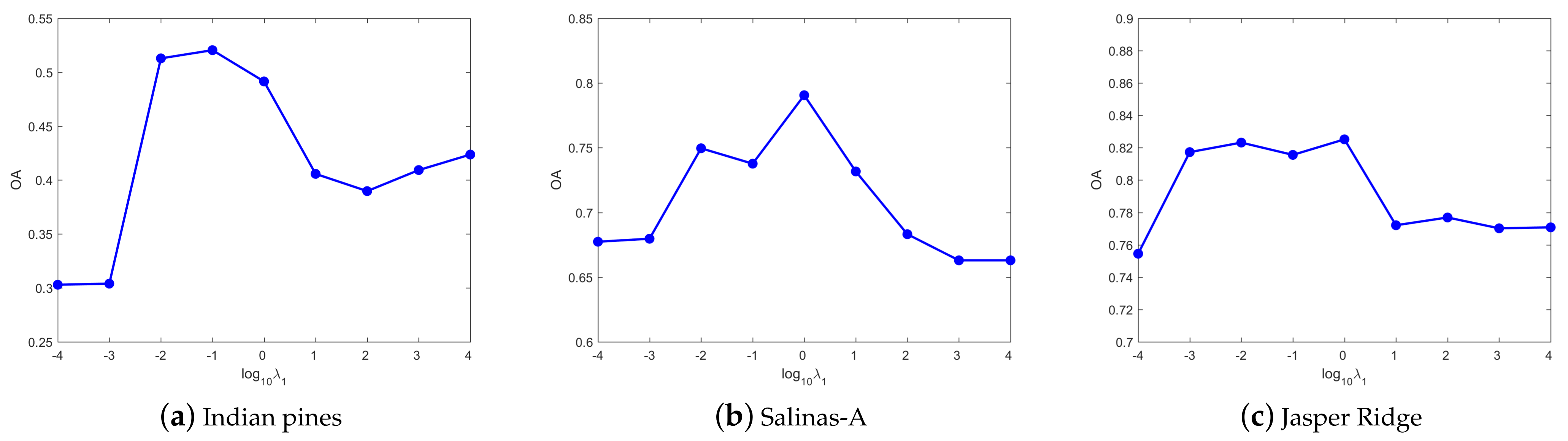
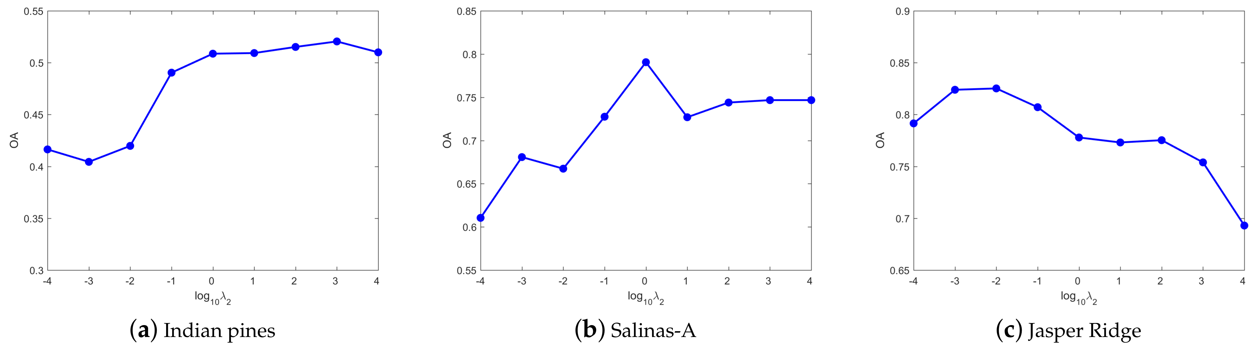
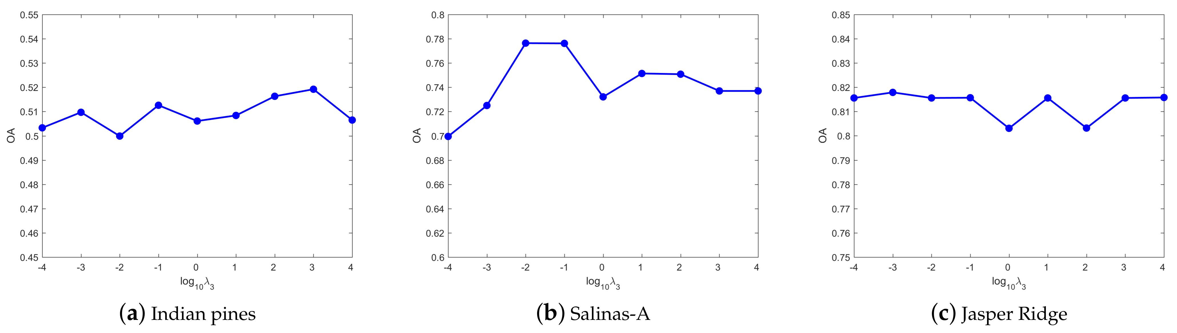
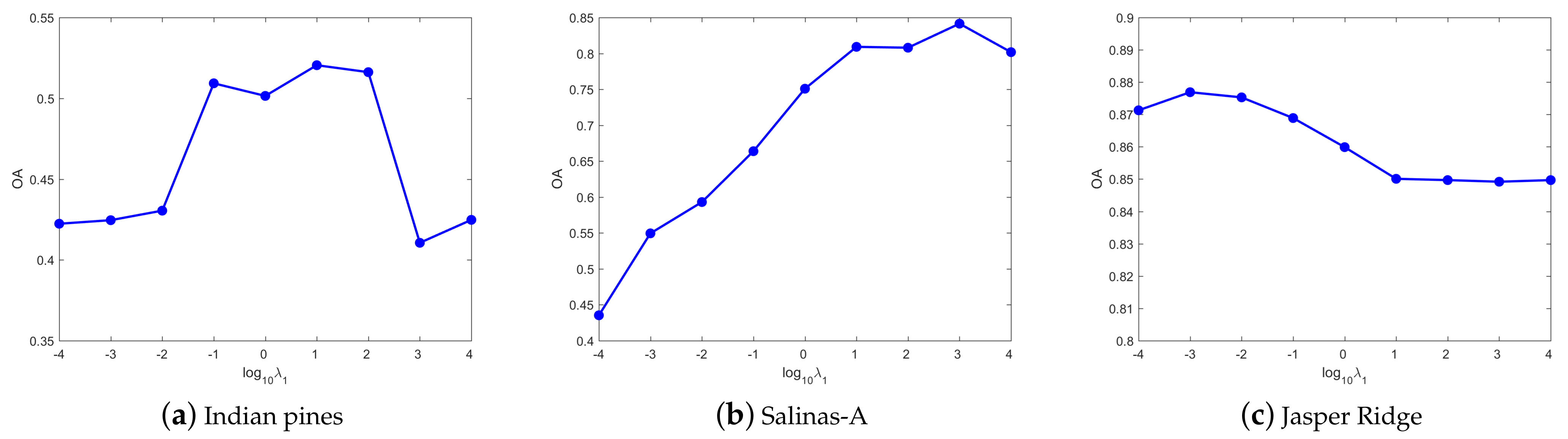
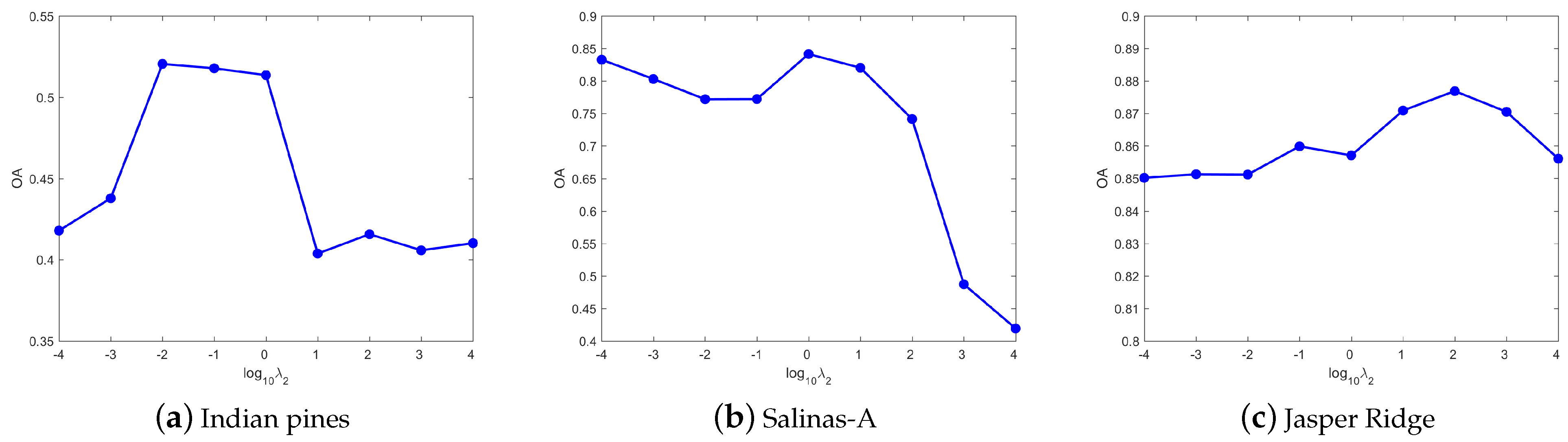
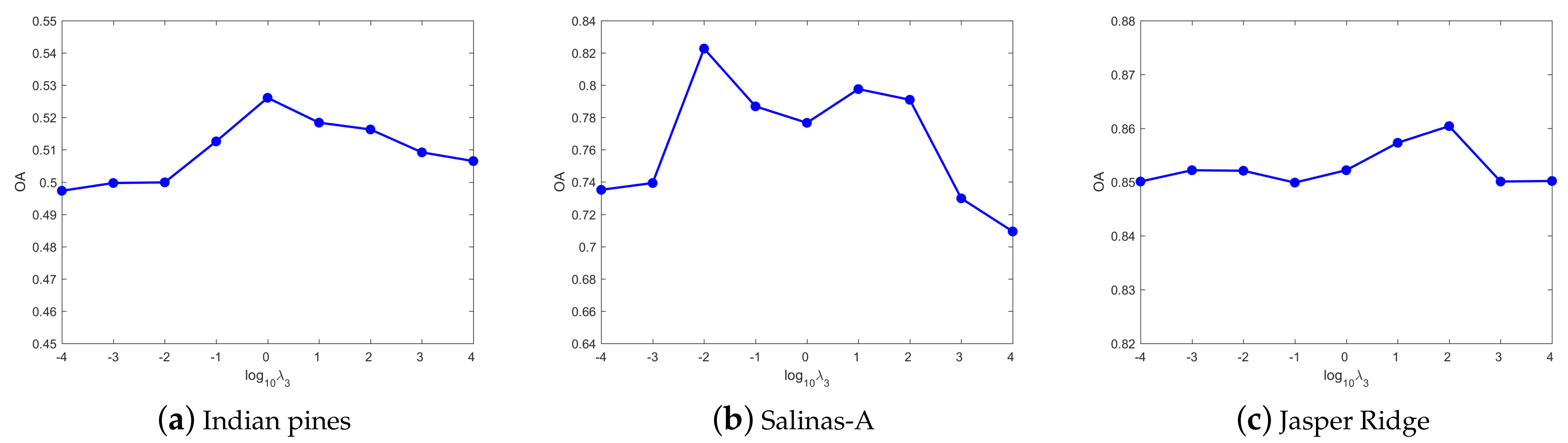
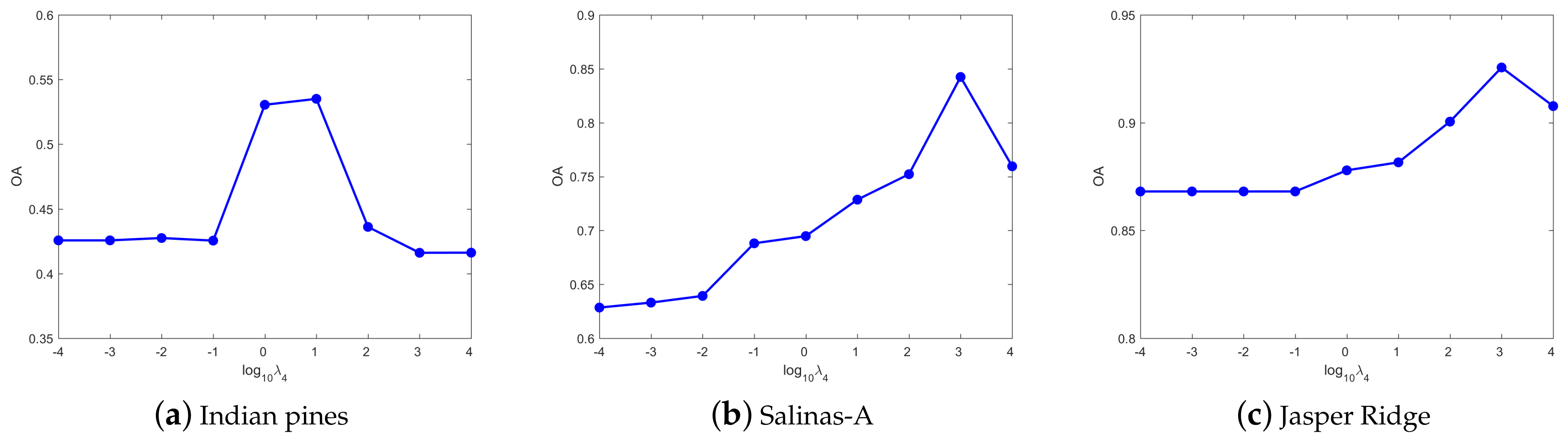
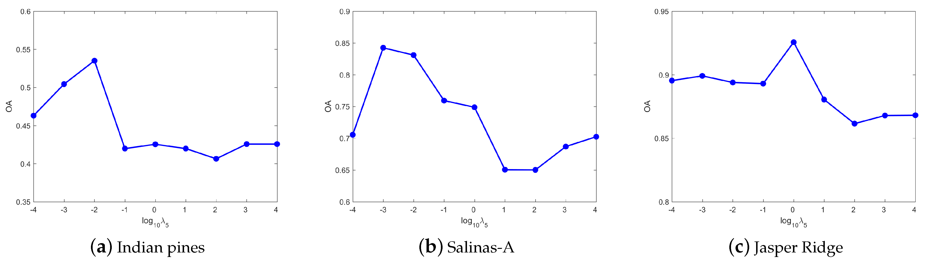
4.3. Parameters Tuning

There are five parameters ${\lambda }_1$, ${\lambda }_2$, ${\lambda }_3$, ${\lambda }_4$, and ${\lambda }_5$ in UDHLR, and three parameters ${\lambda }_1$, ${\lambda }_2$, ${\lambda }_3$ in DHLR. In this section, we evaluate the parameter sensitivity of the proposed methods on three datasets, and investigate different parameter settings. In the experiment, we tune the parameters ${\lambda }_1$, ${\lambda }_2$, ${\lambda }_3$, ${\lambda }_4$, and ${\lambda }_5$ in the range of $\left\{{10}^{-4},{10}^{-3},{10}^{-2},{10}^{-1},1,{10}^1,{10}^2,{10}^3,{10}^4\right\}$. We observe the variations of OA with different values of each parameters.

(1) Parameter analysis in DHLR: In DHLR, ${\lambda }_1$ is the manifold regularization parameter, ${\lambda }_2$ is the noise regularization parameter, ${\lambda }_3$ is penalty parameter of hyperedge weight $\mathbf{W}$. Figure 3 shows the OA of DHLR with respect to the parameter ${\lambda }_1$. For the Indian Pines dataset, the peak value of OA generates when ${\lambda }_1=0.1$. For the Salinas-A dataset, we set ${\lambda }_1=1$ for obtaining the best result in the experiments. For the Jasper Ridge dataset, the clustering results are better when we set ${\lambda }_1=1$. Figure 4 shows the OA of DHLR with respect to the parameter ${\lambda }_2$. For the Indian Pines dataset, the peak value of OA generates when ${\lambda }_2=1000$. For the Salinas-A dataset, we set ${\lambda }_2=1$ for obtaining the best result in the experiments. For the Jasper Ridge dataset, the clustering results are better when we set ${\lambda }_2=0.01$. Figure 5 shows the OA of DHLR with respect to the parameter ${\lambda }_3$. According to Figure 5, we find that the proposed methods can achieve better performance with ${\lambda }_3$ in the setting of 1000, 0.01, 0.001 for the Indian Pines, Salinas-A, and Jasper Ridge datasets, respectively.

(2) Parameter analysis in UDHLR: Except for the same three parameters ${\lambda }_1$, ${\lambda }_2$, and ${\lambda }_3$ as DHLR, ${\lambda }_4$ is the parameter of the label feature manifold regularization. In addition, ${\lambda }_5$ is conductive to discrete label learning. Figure 6 shows the OA of UDHLR with respect to the parameters ${\lambda }_1$. For the Indian Pines dataset, the best results can be achieved when ${\lambda }_1=10$. For the Salinas-A dataset, the clustering results are better when we set ${\lambda }_1=1000$. For the Jasper Ridge dataset, we set ${\lambda }_1=0.001$ for obtaining the best result in the experiments. Figure 7 shows the OA of UDHLR with respect to the parameters ${\lambda }_2$. For the Indian Pines dataset, the best results can be achieved when ${\lambda }_2=0.01$. For the Salinas-A dataset, the clustering results are better when we set ${\lambda }_2=1$. For the Jasper Ridge dataset, we set ${\lambda }_2=100$ for obtaining the best result in the experiments. Figure 8 shows the OA of UDHLR with respect to the parameters ${\lambda }_3$. The UDHLR performs well when ${\lambda }_3$ being set of 1, 0.01, 100 for the Indian Pines, Salinas-A, and Jasper Ridge datasets, respectively. In UDHLR, ${\lambda }_4$ and ${\lambda }_5$ play a vital role in clustering performance. Figure 9 demonstrates the OA values of three datasets under tuning ${\lambda }_4$ while keeping other parameters fixed. As can be seen, the best result can be achieved when ${\lambda }_4=10$ for the Indian Pines dataset. For the Salinas-A dataset, we set ${\lambda }_4=1000$ in our experiments. The results in Figure 9c show that the UDHLR performs well when ${\lambda }_4=1000$ for the Jasper Ridge dataset. Figure 10 shows the OA of UDHLR with respect to the parameters ${\lambda }_5$. For the Indian Pines dataset, the peak value of OA generates when ${\lambda }_5=0.01$. For the Salinas-A dataset, we set ${\lambda }_5=0.001$ for obtaining the best result in the experiments. For the Jasper Ridge dataset, the clustering results are better when we set ${\lambda }_5=1$.

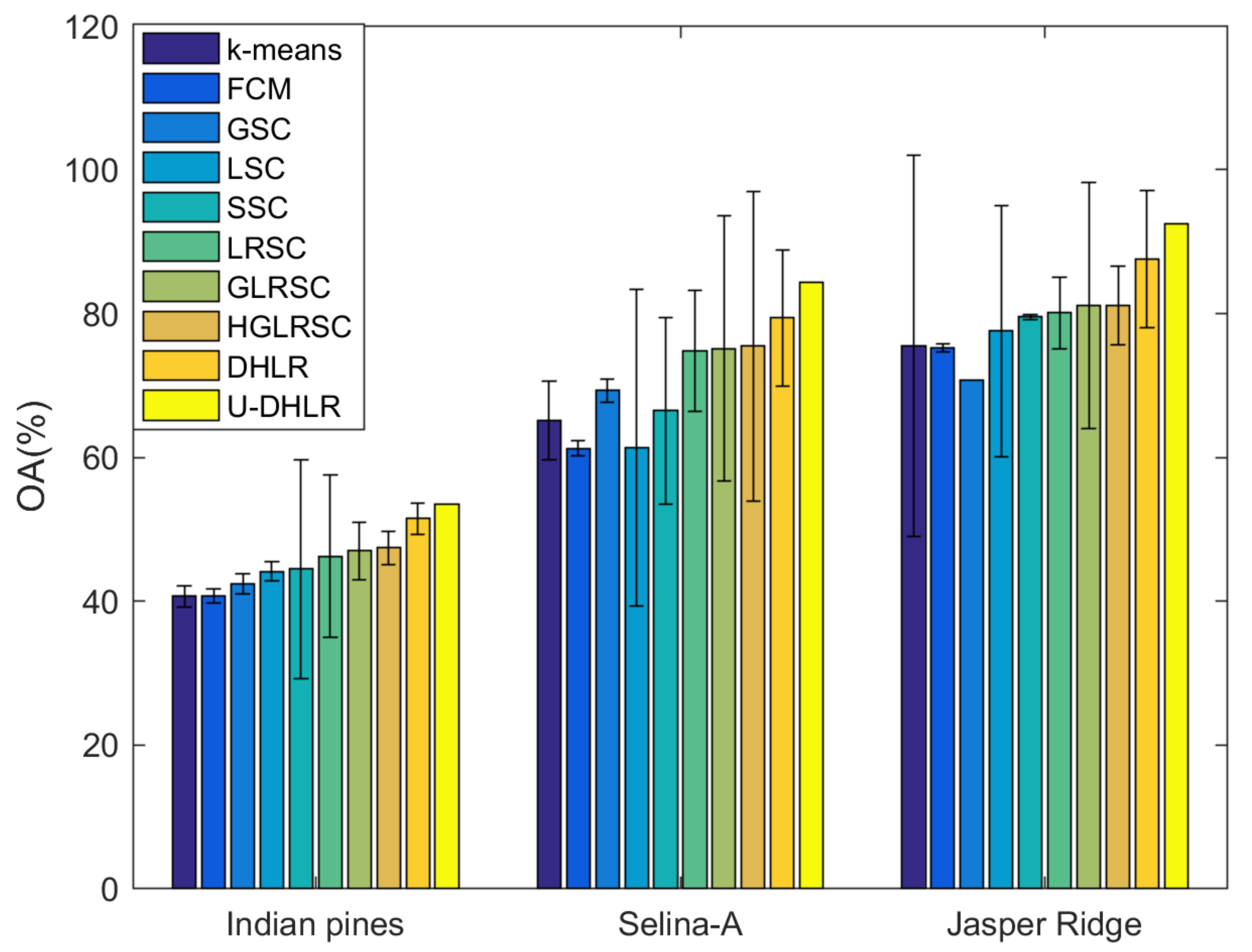
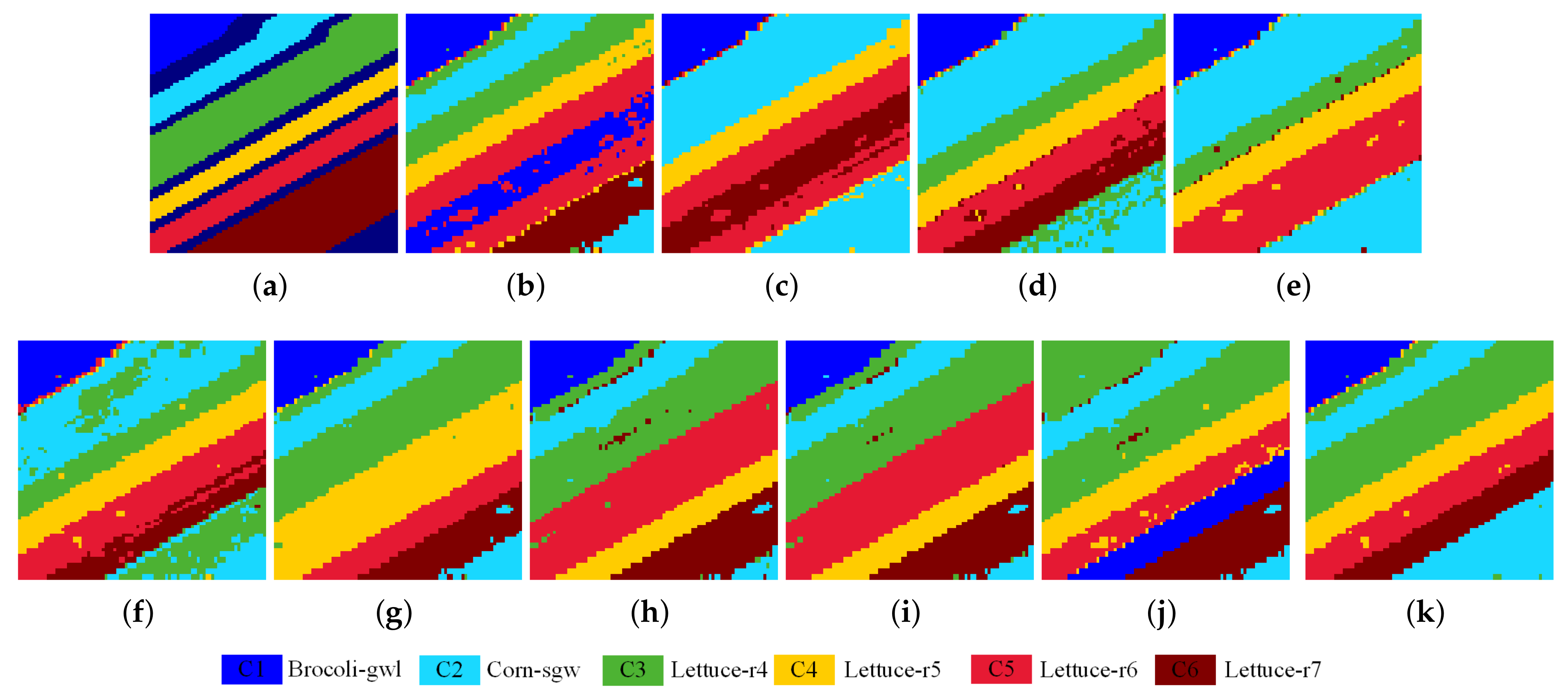
4.4. Investigate of Clustering Performance

Both the clustering maps and quantitative evaluation results are given in this section. The presented results clearly demonstrate that DHLR and UDHLR outperform the other methods on the three datasets. We run all the methods 100 times independently, and show the mean results of the clustering result in the corresponding Tables of the three datasets. In addition, the corresponding variance values of the methods generated in three datasets are recorded in Figure 11.

(1) Indian Pines: Figure 12 shows the clustering maps of the Indian Pines dataset.

Table 3. Performance of Indian Pines dataset.

IP	Class	Method
	No.	k-Means	FCM	GSC	LSC	SSC	LRSC	GLRSC	HGLRSC	DHLR	UDHLR
User’s accuracy (%)	C1	26.50	42.61	29.15	11.16	56.97	56.97	56.90	23.84	00.55	0.62
	C2	0.00	15.83	0.00	0.00	0.00	0.00	0.00	0.35	0.00	0.00
	C3	7.04	12.27	18.51	4.63	28.77	6.04	44.26	57.34	65.79	65.79
	C4	40.70	35.48	31.73	30.12	88.35	95.85	90.22	76.43	83.93	87.81
	C5	99.39	98.98	91.41	99.59	99.80	100	99.79	99.59	99.59	99.59
	C6	17.46	31.51	0.00	4.24	0.00	0.72	0.72	0.61	50.20	0.72
	C7	66.05	43.56	73.95	88.86	45.87	45.87	46.23	81.28	59.92	85.61
	C8	0.49	0.00	27.52	0.00	31.11	30.78	31.92	0.32	41.20	42.50
	C9	61.28	67.23	59.35	76.89	56.11	72.72	65.45	56.10	88.17	88.17
Producer’s accuracy (%)	C1	23.39	31.17	30.13	27.35	27.98	27.98	28.20	22.55	21.05	22.50
	C2	0.00	14.66	0.00	0.00	0.00	0.00	0.00	2.63	0.00	0.00
	C3	6.27	17.13	26.13	17.42	50.88	11.53	31.65	35.62	93.42	93.96
	C4	80.21	88.92	86.49	90.00	89.30	72.91	78.92	80.19	83.15	81.38
	C5	63.36	64.79	71.86	49.74	99.18	90.72	96.06	84.25	100	100
	C6	18.15	21.52	0.00	25.30	0.00	12.50	12.50	12.76	24.01	2.80
	C7	43.87	53.80	44.11	39.67	43.70	43.48	43.69	42.30	41.90	40.57
	C8	60.00	0.00	21.91	0.00	25.67	25.36	25.42	100	24.80	24.53
	C9	72.88	73.85	73.00	75.78	69.40	75.94	88.69	87.05	100	100
OA (%)		40.66	40.70	42.33	44.13	44.48	46.24	46.96	47.38	51.45	53.52
AA (%)		35.43	38.61	36.85	35.05	45.22	45.44	48.39	43.99	54.37	52.32
$\kappa$		0.284	0.308	0.299	0.303	0.341	0.361	0.372	0.353	0.423	0.429
NMI (%)		43.08	41.17	43.55	46.68	47.28	45.31	46.12	46.58	48.68	54.26

gives the quantitative the clustering results. In general, the graph-based methods get better performance than the methods with no graph. Specifically, the K-means and FCM methods perform poorly with many misclassifications in the cluster map because of without exploring the local geometrical structure of the data. Compared with K-means and FCM, the GSC and LSC methods improves the clustering results by applying k-means on the eigenspace of the Laplacian matrices. In contrast, the subspace clustering methods can obtain a much better performance by using subspace learning to model the complex inherent structure of HSI data. Compared with K-means, SSC and LRSC perform much better in this dataset, obtaining the increments in OA of 3.82% and 5.58%, respectively. However, the learned representation coefficient matrix cannot capture the essential geometric structure information. As a result, the clustering results are not very high. GLRSC and HGLRSC improve the clustering performance of LRSC by optimizing the low-rank representation coefficient with the graph and hypergraph regularization, which shows the advantage of incorporating the latent geometric structure information. Unfortunately, the hypergraph is usually fixed, which is constructed by the original data, which is not optimized adaptively. The proposed DHLR algorithm improves 4.49% compared with the classical LRSC, and more than 4.07% compared with HGLRSC. Furthermore, the proposed UDHLR method obtains the best results with the 2.07% improvements than DHLR.

(2) Salinas-A: Figure 13 illustrates the visualization performance of the Salinas-A dataset.

Table 4. Performance of Salinas-A dataset.

IP	Class	Method
	No.	k-means	FCM	GSC	LSC	SSC	LRSC	GLRSC	HGLRSC	DHLR	UDHLR
User’s accuracy (%)	C1	0.00	99.74	100	99.74	99.48	99.74	99.48	99.48	0.00	99.74
	C2	92.85	0.00	100	0.00	62.50	94.48	87.98	89.28	90.58	92.04
	C3	53.83	48.06	49.63	46.62	54.03	99.86	97.70	99.27	98.22	100
	C4	100	99.85	99.40	99.85	99.85	0.00	0.00	0.00	99.85	99.70
	C5	87.23	95.11	92.86	95.11	98.12	99.74	99.37	99.24	90.48	97.49
	C6	53.53	53.46	39.38	55.69	37.30	52.71	59.86	58.74	59.04	42.88
Producer’s accuracy (%)	C1	0.00	100	100	100	100	100	100	100	0.00	100
	C2	94.23	0.00	33.02	0.00	30.55	88.58	95.59	96.49	96.20	42.53
	C3	94.15	89.28	70.35	97.26	50.30	97.19	96.06	95.94	77.77	96.76
	C4	52.41	55.66	98.82	90.57	96.69	0.00	0.00	0.00	89.85	97.39
	C5	63.42	94.88	98.01	58.64	90.74	54.47	54.68	54.38	99.86	99.74
	C6	100	33.75	91.04	34.45	100	100	93.16	97.04	95.77	99.65
OA (%)		65.12	61.21	69.27	61.36	66.49	74.79	75.15	75.45	79.37	84.31
AA (%)		64.57	66.04	80.21	66.17	75.21	74.42	74.07	74.34	73.03	88.64
$\kappa$		0.582	0.515	0.631	0.517	0.589	0.689	0.691	0.696	0.742	0.808
NMI (%)		70.84	62.67	67.64	63.88	64.38	84.02	81.69	83.33	81.10	86.30

gives the corresponding quantitative clustering results. Among these comparison algorithms, GLRSC and HGLRSC combine the graph theory and representation learning into the HSI data clustering. Meanwhile, SSC and LRSC only use the representation learning to obtain the new feature, and GSC and LSC only use the graph theory into the clustering. It can be seen from Table 4 that clustering accuracy of GSC, LSC, SSC and LRSC is lower than GLRSC and HGLRSC. This indicates that learning with the local geometry structure information can improve the HSI clustering observably. In addition, K-means and FCM methods perform poorer than the spectral-based methods. Compared with the aforementioned methods, the proposed DHLR and UDHLR effectively improve the clustering performance by optimal the hypergraph adaptively. As shown in Table 4, UDHLR achieves the highest OA than other methods. We can see that the proposed DHLR and UDHLR algorithms can effectively preserve the detailed structure information, and show an obvious advantage compared with the other clustering methods.

(3) Jasper Ridge: Figure 14 and

Table 5. Performance of Jasper Ridge dataset.

IP	Class	Method
	No.	k-means	FCM	GSC	LSC	SSC	LRSC	GLRSC	HGLRSC	DHLR	UDHLR
User’s accuracy (%)	C1	97.39	97.13	56.68	72.17	63.15	95.50	78.07	78.44	95.13	92.38
	C2	59.14	56.22	99.87	99.21	97.92	67.55	90.10	90.01	91.91	100
	C3	90.07	93.28	42.17	79.65	71.49	100	97.40	97.32	97.65	84.22
	C4	0.00	0.00	99.46	0.00	100	0.13	2.52	2.52	1.19	87.38
Producer’s accuracy (%)	C1	93.35	95.38	100	100	99.63	99.88	99.92	100	99.81	92.91
	C2	100	100	98.83	99.90	99.54	100	99.96	99.89	100	95.08
	C3	71.19	71.49	40.94	69.76	58.29	71.94	60.23	60.43	72.13	88.60
	C4	0.00	0.00	34.70	0.00	49.02	0.01	5.47	5.38	2.75	91.26
OA (%)		75.56	75.28	70.75	77.55	79.52	80.12	81.08	81.16	82.89	92.56
AA (%)		61.65	61.66	74.55	62.76	83.14	65.79	67.02	67.07	68.33	90.99
$\kappa$		0.662	0.659	0.606	0.690	0.719	0.723	0.732	0.733	0.757	0.894
NMI (%)		73.56	74.45	70.24	74.48	69.25	78.43	68.72	68.82	71.46	77.18

show the visual and quantitative clustering results of Jasper Ridge dataset, respectively. From Figure 14 and Table 5, we can see that the centroid-based and spectral-based clustering methods—K-means, FCM, GSC, LSC, SSC, and LRSC—achieve poorer clustering performance when compared with the graph and hypergraph combined clustering results. On the contrary, GLRSC obtains a much higher clustering accuracy than LRSC. HGLRSC also obtains higher clustering precision than LRSC and GLRSC. The proposed DHLR and UDHLR algorithm outperform the other state-of-the-art clustering methods significantly. In which the UDHLR method achieves the best clustering results, with the best OA of 92.56%, which again demonstrates the advantage of the proposed algorithm.

5. Discussion

In this section, we will discuss the computation complexity of the proposed DHLR and UDHLR methods. The main computation cost of the DHLR algorithm lies in updating ${\mathbf{J}}^{\mathrm{t}+1}$, ${\mathbf{Z}}^{\mathrm{t}+1}$, ${\mathbf{N}}^{\mathrm{t}+1}$, which need the complexity about $\mathcal{O}\left(n^{2}r\right)$ all of them. As referred in [13], r is the rank of the dictionary with the orthogonal basis of the dictionary data. The updating of ${\mathbf{H}}^{\mathrm{t}+1}$ need to construct an $n\times n$ matrix, whose time complexity is $\mathcal{O}\left(n{d}^2\right)$. The complexity of updating ${\mathbf{W}}^{\mathrm{t}+1}$ is $\mathcal{O}\left(n{d}^2\right)$. In addition, updating the Lagrange multipliers take the complexity of $\mathcal{O}\left(nd\right)$, which is too small to be neglected. The complexity of the UDHLR algorithm comes from the updating of ${\mathbf{F}}^{\mathrm{t}+1}$, ${\mathbf{Q}}^{\mathrm{t}+1}$, ${\mathbf{Y}}^{\mathrm{t}+1}$, except for the variables ${\mathbf{J}}^{\mathrm{t}+1}$, ${\mathbf{Z}}^{\mathrm{t}+1}$, ${\mathbf{N}}^{\mathrm{t}+1}$, ${\mathbf{H}}^{\mathrm{t}+1}$, ${\mathbf{W}}^{\mathrm{t}+1}$ same as DHLR. The complexity for updating ${\mathbf{F}}^{\mathrm{t}+1}$ is $\mathcal{O}\left(n{c}^2+c^3\right)$. The solution of solving ${\mathbf{Q}}^{\mathrm{t}+1}$ involves SVD and the complexity is $\mathcal{O}\left(n{c}^2+c^3\right)$. To update ${\mathbf{Y}}^{\mathrm{t}+1}$, we need $\mathcal{O}\left(n{c}^2\right)$. Therefore, the total complexity of UDHLR is $\mathcal{O}\left(n^{2}r+n{d}^2+n{c}^2+c^3\right)$. Though, the number of the cluster c is small, the computation complexity of the proposed methods is greatly higher than original LRSC algorithm because of involving matrix inversion and SVD. In the future, we will consider parallel computing to increasing running speed.

6. Conclusions

In this paper, we propose a novel unified adaptive hypergraph-regularized low-rank subspace learning method for hyperspectral clustering. In the proposed framework, low-rank and the hypergraph terms are used to explore the local and global structure information of data, and the last two terms are used to learn the continuous label and the discrete label. Specifically, the hypergraph is adaptively learned from the low-rank subspace feature without exploring a fixed incidence matrix, which is theoretically optimal for clustering. Otherwise, the proposed model learns a rotation matrix to simultaneously learn continuous labels and discrete cluster labels, which need no relaxing information loss as many existing spectral clustering methods. It jointly learns the similarity hypergraph from the learned low-rank subspace data and the discrete clustering labels by solving an optimization problem, in which the subspace feature is adaptively learned by considering the clustering performance and the continuous clustering labels just serve as intermediate products. The experimental results demonstrate that the proposed DHLR and UDHLR outperforms the existing clustering methods. However, the computational complexity of each iteration is very high in the proposed methods, which should be optimized in the view of running time. In the future, we will optimize the complexity of the proposed method and intend the hypergraph learning to conduct the large-scale hyperspectral image clustering.

References

1. Wang, Q.; He, X.; Li, X. Locality and structure regularized low rank representation for hyperspectral image classification. IEEE Trans. Geosci. Remote Sens. 2018, 57, 911–923. [Google Scholar] [CrossRef] [Green Version]
2. Liu, J.; Xiao, Z.; Chen, Y.; Yang, J. Spatial-spectral graph regularized kernel sparse representation for hyperspectral image classification. ISPRS Int. J. Geo-Inform. 2017, 6, 258. [Google Scholar] [CrossRef]
3. Liu, J.; Wu, Z.; Xiao, Z.; Yang, J. Classification of hyperspectral images using kernel fully constrained least squares. ISPRS Int. J. Geo-Inform. 2017, 6, 344. [Google Scholar] [CrossRef] [Green Version]
4. Shen, Y.; Xiao, L.; Chen, J.; Pan, D. A Spectral-Spatial Domain-Specific Convolutional Deep Extreme Learning Machine for Supervised Hyperspectral Image Classification. IEEE Access 2019, 7, 132240–132252. [Google Scholar] [CrossRef]
5. Zhang, H.; Zhai, H.; Zhang, L.; Li, P. Spectral—spatial sparse subspace clustering for hyperspectral remote sensing images. IEEE Trans. Geosci. Remote Sens. 2016, 54, 3672–3684. [Google Scholar] [CrossRef]
6. Lloyd, S. Least squares quantization in PCM. IEEE Trans. Inform. Theory 1982, 28, 129–137. [Google Scholar] [CrossRef]
7. Peizhuang, W. Pattern recognition with fuzzy objective function algorithms (James C. Bezdek). SIAM Rev. 1983, 25, 442. [Google Scholar] [CrossRef]
8. Ng, A.Y.; Jordan, M.I.; Weiss, Y. On spectral clustering: Analysis and an algorithm. In Advances in Neural Information Processing Systems; MIT Press: Vancouver, BC, Canada, 2002; pp. 849–856. [Google Scholar]
9. Belkin, M.; Niyogi, P. Laplacian eigenmaps for dimensionality reduction and data representation. Neur. Comput. 2003, 15, 1373–1396. [Google Scholar] [CrossRef] [Green Version]
10. Elhamifar, E.; Vidal, R. Sparse subspace clustering. In Proceedings of the 2009 IEEE Conference on Computer Vision and Pattern Recognition, Los Alamitos, CA, USA, 20–25 June 2009; pp. 2790–2797. [Google Scholar]
11. Elhamifar, E.; Vidal, R. Sparse subspace clustering: Algorithm, theory, and applications. IEEE Trans. Pattern Anal. Mach. Intell. 2013, 35, 2765–2781. [Google Scholar] [CrossRef] [Green Version]
12. Vidal, R.; Favaro, P. Low rank subspace clustering (LRSC). Pattern Recognit. Lett. 2014, 43, 47–61. [Google Scholar] [CrossRef] [Green Version]
13. Liu, G.; Lin, Z.; Yan, S.; Sun, J.; Yu, Y.; Ma, Y. Robust recovery of subspace structures by low-rank representation. IEEE Trans. Pattern Anal. Mach. Intell. 2012, 35, 171–184. [Google Scholar] [CrossRef] [Green Version]
14. Zheng, M.; Bu, J.; Chen, C.; Wang, C.; Zhang, L.; Qiu, G.; Cai, D. Graph regularized sparse coding for image representation. IEEE Trans. Image Process. 2010, 20, 1327–1336. [Google Scholar] [CrossRef] [PubMed]
15. Lu, X.; Wang, Y.; Yuan, Y. Graph-regularized low-rank representation for destriping of hyperspectral images. IEEE Trans. Geosci. Remote Sens. 2013, 51, 4009–4018. [Google Scholar] [CrossRef]
16. Berge, C. Hypergraphs; North-Holland: Amsterdam, The Netherlands, 1989. [Google Scholar]
17. Zhou, D.; Huang, J.; Schölkopf, B. Learning with hypergraphs: Clustering, classification, and embedding. Adv. Neural Inf. Process. Syst. 2006, 19, 1601–1608. [Google Scholar]
18. Yuan, H.; Tang, Y.Y. Learning with hypergraph for hyperspectral image feature extraction. IEEE Geosci. Remote Sens. Lett. 2015, 12, 1695–1699. [Google Scholar] [CrossRef]
19. Bai, X.; Guo, Z.; Wang, Y.; Zhang, Z.; Zhou, J. Semisupervised hyperspectral band selection via spectral—Spatial hypergraph model. IEEE J. Sel. Top. Appl. Earth Obs. Remote Sens. 2015, 8, 2774–2783. [Google Scholar] [CrossRef] [Green Version]
20. Du, W.; Qiang, W.; Lv, M.; Hou, Q.; Zhen, L.; Jing, L. Semi-supervised dimension reduction based on hypergraph embedding for hyperspectral images. Int. J. Remote Sens. 2018, 39, 1696–1712. [Google Scholar] [CrossRef]
21. Chang, Y.; Yan, L.; Zhong, S. Hyper-laplacian regularized unidirectional low-rank tensor recovery for multispectral image denoising. In Proceedings of the IEEE Conference on Computer Vision and Pattern Recognition, Honolulu, HI, USA, 21–26 July 2017; pp. 4260–4268. [Google Scholar]
22. Huang, H.; Chen, M.; Duan, Y. Dimensionality reduction of hyperspectral image using spatial-spectral regularized sparse hypergraph embedding. Remote Sens. 2019, 11, 1039. [Google Scholar] [CrossRef] [Green Version]
23. Gao, S.; Tsang, I.W.H.; Chia, L.T. Laplacian sparse coding, hypergraph laplacian sparse coding, and applications. IEEE Trans. Pattern Anal. Mach. Intell. 2012, 35, 92–104. [Google Scholar] [CrossRef] [PubMed]
24. Zeng, K.; Yu, J.; Li, C.; You, J.; Jin, T. Image clustering by hyper-graph regularized non-negative matrix factorization. Neurocomputing 2014, 138, 209–217. [Google Scholar] [CrossRef]
25. Wang, W.; Qian, Y.; Tang, Y.Y. Hypergraph-regularized sparse NMF for hyperspectral unmixing. IEEE J. Sel. Top. Appl. Earth Obs. Remote Sens. 2016, 9, 681–694. [Google Scholar] [CrossRef]
26. Yin, M.; Gao, J.; Lin, Z. Laplacian regularized low-rank representation and its applications. IEEE Trans. Pattern Anal. Mach. Intell. 2015, 38, 504–517. [Google Scholar] [CrossRef] [PubMed]
27. Zeng, M.; Ning, B.; Hu, C.; Gu, Q.; Cai, Y.; Li, S. Hyper-Graph Regularized Kernel Subspace Clustering for Band Selection of Hyperspectral Image. IEEE Access 2020, 8, 135920–135932. [Google Scholar] [CrossRef]
28. Zhang, Z.; Bai, L.; Liang, Y.; Hancock, E. Joint hypergraph learning and sparse regression for feature selection. Pattern Recognit. 2017, 63, 291–309. [Google Scholar] [CrossRef] [Green Version]
29. Zhang, Z.; Lin, H.; Gao, Y.; BNRist, K. Dynamic Hypergraph Structure Learning. In Proceedings of the International Joint Conferences on Artificial Intelligence Organization, Stockholm, Sweden, 13–19 June 2018; pp. 3162–3169. [Google Scholar]
30. Zhu, X.; Zhu, Y.; Zhang, S.; Hu, R.; He, W. Adaptive Hypergraph Learning for Unsupervised Feature Selection. In Proceedings of the Twenty-Seventh International Joint Conference on Artificial Intelligence IJCAI, Melbourne, VIC, Australia, 19–25 August 2017; pp. 3581–3587. [Google Scholar]
31. Zhu, X.; Zhang, S.; Zhu, Y.; Zhu, P.; Gao, Y. Unsupervised Spectral Feature Selection with Dynamic Hyper-graph Learning. IEEE Trans. Knowl. Data Eng. 2020. [Google Scholar] [CrossRef]
32. Tang, C.; Liu, X.; Wang, P.; Zhang, C.; Li, M.; Wang, L. Adaptive hypergraph embedded semi-supervised multi-label image annotation. IEEE Trans. Multimed. 2019, 21, 2837–2849. [Google Scholar] [CrossRef]
33. Ding, D.; Yang, X.; Xia, F.; Ma, T.; Liu, H.; Tang, C. Unsupervised feature selection via adaptive hypergraph regularized latent representation learning. Neurocomputing 2020, 378, 79–97. [Google Scholar] [CrossRef]
34. Kang, Z.; Peng, C.; Cheng, Q.; Xu, Z. Unified Spectral Clustering with Optimal Graph. In Proceedings of the Thirty-First AAAI Conference on Artificial Intelligence (AAAI-17), San Francisco, CA, USA, 4–9 February 2017. [Google Scholar]
35. Han, Y.; Zhu, L.; Cheng, Z.; Li, L.; Liu, X. Discrete Optimal Graph Clustering. IEEE Trans. Cybernet. 2020, 50, 1697–1710. [Google Scholar] [CrossRef] [Green Version]
36. Yang, Y.; Shen, F.; Huang, Z.; Shen, H.T. A Unified Framework for Discrete Spectral Clustering. In Proceedings of the Twenty-Fifth International Joint Conference on Artificial Intelligence, Phoenix, AZ, USA, 12–17 February 2016; pp. 2273–2279. [Google Scholar]
37. Lin, Z.; Chen, M.; Ma, Y. The Augmented Lagrange Multiplier Method for Exact Recovery of Corrupted Low-Rank Matrices. arXiv 2010, arXiv:1009.5055. [Google Scholar]
38. Liu, G.; Yan, S. Latent Low-Rank Representation for subspace segmentation and feature extraction. In Proceedings of the 2011 International Conference on Computer Vision, Barcelona, Spain, 6–13 November 2011; pp. 1615–1622. [Google Scholar] [CrossRef]
39. Boley, D.; Chen, Y.; Bi, J.; Wang, J.Z.; Huang, J.; Nie, F.; Huang, H.; Rahimi, A.; Recht, B. Spectral Rotation versus K-Means in Spectral Clustering. In Proceedings of the Twenty-Seventh AAAI Conference on Artificial Intelligence, Bellevue, WA, USA, 14–18 July 2013. [Google Scholar]
40. Kang, Z.; Peng, C.; Cheng, Q. Twin Learning for Similarity and Clustering: A Unified Kernel Approach. In Proceedings of the Thirty-First AAAI Conference on Artificial Intelligence (AAAI-17), San Francisco, CA, USA, 4–9 February 2017. [Google Scholar]
41. Mohar, B. The Laplacian spectrum of graphs. In Graph Theory, Combinatorics, and Applications; Wiley: Hoboken, NJ, USA, 1991; pp. 871–898. [Google Scholar]
42. Fan, K. On a Theorem of Weyl Concerning Eigenvalues of Linear Transformations I. Proc. Natl. Acad. Sci. USA 1949, 35, 652–655. [Google Scholar] [CrossRef] [Green Version]
43. Yu, S.X.; Shi, J. Multiclass Spectral Clustering. In Proceedings of the IEEE International Conference on Computer Vision, Nice, France, 13–16 October 2003. [Google Scholar]
44. Wen, Z.; Yin, W. A feasible method for optimization with orthogonality constraints. Math. Programm. 2013, 142, 397–434. [Google Scholar] [CrossRef] [Green Version]
45. Nie, F.; Zhang, R.; Li, X. A generalized power iteration method for solving quadratic problem on the Stiefel manifold. Sci. China Inf. Sci. 2017, 60, 112101. [Google Scholar] [CrossRef]
46. Zhong, Y.; Zhang, L.; Gong, W. Unsupervised remote sensing image classification using an artificial immune network. Int. J. Remote Sens. 2011, 32, 5461–5483. [Google Scholar] [CrossRef]
47. Ji, R.; Gao, Y.; Hong, R.; Liu, Q. Spectral-Spatial Constraint Hyperspectral Image Classification. IEEE Trans. Geosci. Remote Sens. 2014, 3, 1811–1824. [Google Scholar] [CrossRef]
48. Ul Haq, Q.S.; Tao, L.; Sun, F.; Yang, S. A Fast and Robust Sparse Approach for Hyperspectral Data Classification Using a Few Labeled Samples. Geosci. Remote Sens. IEEE Trans. 2012, 50, 2287–2302. [Google Scholar] [CrossRef]
49. Strehl, A.; Ghosh, J. Cluster Ensembles—A Knowledge Reuse Framework for Combining Multiple Partitions. J. Mach. Learn. Res. 2002, 3, 583–617. [Google Scholar]
50. Lovasz, L.; Plummer, M.D. Matching Theory; AMS Chelsea Publishing: Amsterdam, North Holland, 1986. [Google Scholar]
51. Murphy, J.M.; Maggioni, M. Unsupervised Clustering and Active Learning of Hyperspectral Images with Nonlinear Diffusion. IEEE Trans. Geosci. Remote Sens. 2019, 57, 1829–1845. [Google Scholar] [CrossRef] [Green Version]
52. Xu, J.; Fowler, J.E.; Xiao, L. Hypergraph-Regularized Low-Rank Subspace Clustering Using Superpixels for Unsupervised Spatial-Spectral Hyperspectral Classification. IEEE Geosci. Remote Sens. Lett. 2020, 1–5. [Google Scholar] [CrossRef]
Figure 1. Illustration of the proposed method.
Remotesensing 13 01372 g001
Figure 2. Illustration of updating the dynamic hypergraph.
Remotesensing 13 01372 g002
Figure 3. The OA of DHLR with different λ 1 on three datasets.
Remotesensing 13 01372 g003
Figure 4. The OA of DHLR with different λ 2 on three datasets.
Remotesensing 13 01372 g004
Figure 5. The OA of DHLR with different λ 3 on three datasets.
Remotesensing 13 01372 g005
Figure 6. The OA of UDHLR with different λ 1 on three datasets.
Remotesensing 13 01372 g006
Figure 7. The OA of UDHLR with different λ 2 on three datasets.
Remotesensing 13 01372 g007
Figure 8. The OA of UDHLR with different λ 3 on three datasets.
Remotesensing 13 01372 g008
Figure 9. The OA of UDHLR with different λ 4 on three datasets.
Remotesensing 13 01372 g009
Figure 10. The OA of UDHLR with different λ 5 on three datasets.
Remotesensing 13 01372 g010
Figure 11. Histogram of the clustering accuracy with variance.
Remotesensing 13 01372 g011
Figure 12. Indian Pines dataset. (a) Ground-truth. (b) k-means, 40.66%. (c) FCM, 40.70%. (d) GSC, 42.33%. (e) LSC, 44.13%. (f) SSC, 44.48%. (g) LRSC, 46.24%. (h) GLRSC, 46.86%. (i) HGLRSC, 47.38%. (j) DHLR, 51.45%. (k) UDHLR, 53.52%.
Remotesensing 13 01372 g012
Figure 13. Salinas-A dataset. (a) Ground-truth. (b) k-means, 65.12%. (c) FCM, 61.21%. (d) GSC, 69.27%. (e) LSC, 61.36%. (f) SSC, 66.49%. (g) LRSC, 74.79%. (h) GLRSC, 75.15%. (i) HGLRSC, 75.45%. (j) DHLR, 79.37%. (k) UDHLR, 84.31%.
Remotesensing 13 01372 g013
Figure 14. Jasper Ridge dataset. (a) Ground-truth. (b) k-means, 75.56%. (c) FCM, 75.28%. (d) GSC, 70.75%. (e) LSC, 77.55%. (f) SSC, 79.52%. (g) LRSC, 80.12%. (h) GLRSC, 81.09%. (i) HGLRSC, 81.16%. (j) DHLR, 82.89%. (k) UDHLR, 92.56%.
Remotesensing 13 01372 g014