Snake-Based Model for Automatic Roof Boundary Extraction in the Object Space Integrating a High-Resolution Aerial Images Stereo Pair and 3D Roof Models

Abstract

The accelerated urban development over the last decades has made it necessary to update spatial information rapidly and constantly. Therefore, cities’ three-dimensional models have been widely used as a study base for various urban problems. However, although many efforts have been made to develop new building extraction methods, reliable and automatic extraction is still a major challenge for the remote sensing and computer vision communities, mainly due to the complexity and variability of urban scenes. This paper presents a method to extract building roof boundaries in the object space by integrating a high-resolution aerial images stereo pair, three-dimensional roof models reconstructed from light detection and ranging (LiDAR) data, and contextual information of the scenes involved. The proposed method focuses on overcoming three types of common problems that can disturb the automatic roof extraction in the urban environment: perspective occlusions caused by high buildings, occlusions caused by vegetation covering the roof, and shadows that are adjacent to the roofs, which can be misinterpreted as roof edges. For this, an improved Snake-based mathematical model is developed considering the radiometric and geometric properties of roofs to represent the roof boundary in the image space. A new approach for calculating the corner response and a shadow compensation factor was added to the model. The created model is then adapted to represent the boundaries in the object space considering a stereo pair of aerial images. Finally, the optimal polyline, representing a selected roof boundary, is obtained by optimizing the proposed Snake-based model using a dynamic programming (DP) approach considering the contextual information of the scene. The results showed that the proposed method works properly in boundary extraction of roofs with occlusion and shadows areas, presenting completeness and correctness average values above 90%, RMSE average values below 0.5 m for E and N components, and below 1 m for H component.

1. Introduction

In the last decades, urban development has been happening at an accelerated rate, making it necessary for the constant and rapid updating of spatial information. However, the big challenge remains in providing high-quality information to enable advanced geospatial processing and support collaborative problem solving [1]. In this sense, the three-dimensional models of cities have been widely used as a study base for various urban problems such as pollution modeling and visualization, cadastral updates, building volume estimation, urban planning, and design of communication networks [2].

The three-dimensional reconstruction of buildings, which are fundamental for constructing three-dimensional models of cities, mainly involves the steps of detection, extraction of the boundary, and reconstruction of roofs. Many efforts have been made in recent decades to develop new building extraction methods, but reliable and automatic extraction remains a challenge for the remote sensing and computer vision communities due to the complexity and variability of urban scenes [3].

The process of extracting roof boundaries from aerial images can be hampered by contextual conditions present in the scenes that can hinder the work of the extraction algorithm. In urban environments, the main contextual configurations that may cause these problems are:

• Vegetation that rises above roofs, partially or totally obstructing their faces. The main problem of this type of obstruction is the lack of radiometric response along roof edges and corners. However, the rectilinear geometry of the roof can be used to overcome the obstruction problem;
• Shadows adjacent to the roof edges, caused by the roof itself and the sunlight projection. In this case, the shadow edge gradients are usually higher than the roof edge gradients; as a result, the shadow edges can be misinterpreted as a roof boundary. However, the gradient vector itself can be used to weight the edge responses;
• Viewpoint-dependent obstructions caused by adjacent buildings. In urban area images, it is common for building roofs to appear obstructed by neighboring building, depending on the viewpoints of the image taking. However, it is possible to explore the fact that obstructed parts in one image may be visible in the other image of a stereo pair, allowing the correct extraction of the roof boundaries.

Several building extraction methods have been reported due to the emergence of different remote sensing technology over the last few decades. For example, aerial images have been used in many works to extract buildings [4,5,6,7], but they face many problems due to occlusions, shadows, and disadvantageous image perspectives [8]. On the other hand, other works [9,10,11,12] have proposed the use of light detection and ranging (LiDAR) data to exploit the 3D information for building extraction. However, the boundaries’ accuracy in these cases can be compromised due to the LiDAR point cloud sparsity. Therefore, many authors have explored the synergy between aerial images and LiDAR data to improve the building extraction process [3,13,14,15,16]. Nevertheless, the efficient integration of these two data sources for building extraction still needs improvement.

The International Society for Photogrammetry and Remote Sensing (ISPRS) reports that even though the 3D object reconstruction from images and point clouds has reached good outcomes in research, some problems still persist. Hence, the integration of image matching, tracking of patterns, and object extraction in the same process is a potential solution to these problems [1]. Thus, in this work, we propose integrating the processes of matching and 3D roof tracing.

Among the enormous efforts that have been made to extract building boundaries from remote sensing data, the Snake model, or active contour model, is a widely used technique. This model is a curve extracting method based on the idea of minimizing energy guided by internal forces within the curve itself and other external forces. In the work of Chen et al. [17], an improved Snake model was proposed to refine the initial boundaries of buildings extracted from LiDAR data. First, a Snake model was built with deviation angle, image gradient, and area constraints. Then, the boundary nodes were moved to find the best result using a greedy algorithm. The authors emphasized that the interference from vegetation, shadow and the edge features on the building boundary may affect the method results, but this problem was not addressed by the work. Sun et al. [18] proposed two strategies for combining convolutional neural networks (CNN) and the Snake model to extract building boundaries. The first strategy was to extract the building boundaries by integrating the Snake model into CNN construction progress, and the second strategy was to use CNN for initial building detection and then apply the Snake model for post-processing. As highlighted in the paper, despite the good results, the method showed poor results in the case of buildings with vegetation on the roof. Although the authors do not delve into this problem, they report that this is due to the difference in the data distribution between the training data and the experiments scenes. Griffiths and Boehm [19] present a method to increase the quality of low-precision large data sets used to train segmentation networks. The Morphological Geodesic Active Contours (MorphGAC) is used to trace the building edge and perform an accurate segmentation. The segmented image is then used as training data for application in CNN. The main disadvantage of MorphoGACs is the need for strong edges, making it necessary to use gradient images, for example. Nguyen et al. [8] presented the super-resolution-based Snake model (SRSM) for large-scale building extraction. The SRSM operates on LiDAR-based elevation images moving the Snake curve adaptively based on a pre-provided building mask. However, they faced the problem of extracted buildings with rounded corners, which is a common situation to the SRSM. The works presented above faced problems related to high vegetation over the roof, shadow, and corner issues in the context of roof extraction. As can be seen in this paper, our method proposes new strategies to minimize these problems and is considered an improvement to the Snake-based mathematical model.

This work presents a methodology to automatically extract the roof boundaries of buildings in 3D, integrating into a single function a stereo pair of high-resolution aerial images, three-dimensional roof models, and contextual information of the scenes involved. For this, a mathematical model was developed based on the Snake theory to model the boundary (characterized by step edges and corners) of the roof. A new approach for calculating the corner response is presented, combining the radiometric and geometric information of the candidate points to a corner. In addition, a shadow compensation factor was added in the calculation of the edge response to attenuate the edge energy resulting from the shadow projected by the building itself, which runs parallel and close to the roof edge and that can cause a false positive. The roof boundaries are extracted by optimizing the energy function created (i.e., the mathematical model of roofs) using a Dynamic Programming (DP) approach. This energy function integrates contextual information of viewpoint-dependent occlusions, shadow, and high vegetation obstructions. The solution obtained—i.e., a polyline representing each 3D roof boundary—will be a higher accurate representation for the correspondent boundary of the 3D roof model.

The main contributions of this work are: (1) the proposal for a new approach for extracting roof boundaries based on the integration between the processes of matching—between roof edge points that belong to two stereo images—and 3D roof tracing, which has been the focus of studies in recent years [1]; (2) the possibility of dealing with viewpoint-dependent obstructions—known as occlusions; (3) the incorporation of mechanisms to overcome typical problems when it comes to extracting roof boundaries in urban environments, namely: obstructions caused by vegetation that rises above the roofs, and shadows adjacent to the roofs, which can be misinterpreted as roof edges; and (4) the creation of an improved mathematical model based on the Snake theory containing a new approach for calculating the corner responses and a shadow compensation factor.

2. Proposed Method

Figure 1 shows the flowchart of the proposed method, which can be subdivided into three main procedures: (1) pre-processing for the generation of two auxiliary images (i.e., the vegetation and shadow images) that are used during the optimization process (dashed box 1); (2) formulation of a mathematical model to represent the roof boundaries in the object space using a stereo pair of images (dashed box 2); (3) solution of the mathematical model through DP optimization (dashed box 3). The following sections present the processes involved in each of these procedures.

2.1. Pre-Processing: Generation of Vegetation and Shadow Auxiliary Images

The pre-processing procedure aims to create two auxiliary images containing: (1) the shadow regions adjacent to the roof; and (2) high vegetation regions. These images are generated with the same size and resolution as the corresponding optical images. Thus, given a pixel in the optical image, it is possible to know if it is in any of these regions of interest and then adapt the parameters of the Snake model to handle each case, as will be described in Section 2.3.1.

It is worth mentioning that in addition to the auxiliary images of vegetation and shadow, the visibility map is also used to solve the Snake model, indicating the regions containing perspective occlusions [20]. Unlike the vegetation and shadow images, the visibility maps were supplied as input data to our method. Figure 2a shows a sample of the visibility map used in this work, where the blue region corresponds to the occluded area, and Figure 2b shows the corresponding aerial image.

2.1.1. Shadow Image

The shadow image shows shadow regions adjacent to the roofs. In order to generate this product, shadows should be detected in aerial images. We used the shadow detection algorithm proposed by Azevedo et al. [21], but with some adaptations as presented below.

Before applying the method proposed by Azevedo et al. [21], we perform a smoothing process to the original image. This is usually necessary because the employed images are of high resolution; as a result, the shadow detection method can identify many unnecessary shadow details caused by small objects, such as the roof tiles. Figure 3a shows an example of a high-resolution aerial image, and Figure 3b shows the detected shadow areas in white. As an example, the Gaussian filter with σ = 2 was chosen to perform the smoothing. Figure 3c presents the detected shadows in the smoothed image and, as it is well-known, many irrelevant details were removed.

After smoothing the image, the first step to detect the shadows is to perform the black top-hat transformation on the smoothed image [22]. This transformation detects the dark patterns in the image through the arithmetic difference between the original image and its closing. As the shadows in aerial images do not obey a specific pattern, the original work by Azevedo et al. [21] uses the area closing operation so that there is no need to establish a particular shape for the structuring element. However, the type of shadow of interest in this work is those cast by the buildings themselves, having rectangular and elongated shapes. Based on these characteristics, the closing operation used in the top-hat transformation is performed using the size 3 “square” structuring element. As a result, an image is created highlighting only the shadows that obey the rectangular and elongated pattern.

The next step is to threshold the image generated by the top-hat transformation. The histogram of the thresholded image has a bimodal behavior, that is, the targets of interest stand out from the other targets in the image. Thus, the Otsu method [23] was chosen to perform the thresholding because it can automatically determine the threshold according to a class separation measure. The result is a two-level image where the shadow pixels have the value 255, and the other pixels have the value 0.

Finally, the morphological area opening operation is applied to the two-level image to eliminate small shadow regions, which can be considered noise. Figure 3d shows the shadow image created by applying the described process.

2.1.2. Vegetation Image

The first step in generating the vegetation image is to determine the regions of high vegetation from the LiDAR data using the software LAStools. For this, a filtering process is used to separate the ground points from the non-ground points (Figure 4a). Then, the regions containing the non-ground points are analyzed individually in order to classify them as vegetation or building (Figure 4b), through the analysis of height, planarity, and roughness of the neighborhood. It is worth mentioning that the filtering and classification processes performed by LAStools are similar to the method presented by [24].

The next step is to project the vegetation points, which are in the LiDAR coordinate system, to the image coordinate system (l, c), using the collinearity equations and image-space transformations (like one that models the lens distortions. For more details on these photogrammetric transformations, please refer to [25,26]).

After the projection of the vegetation points onto the image space, an image is generated, assigning the value 255 to the vegetation pixels and the value 0 to the other pixels (Figure 4c). However, as can be seen in Figure 4c, the vegetation points derived from the LiDAR point cloud are spaced apart and, as such, do not form homogeneous regions in the image. Consequently, it is necessary to carry out some post-processing to fill the spaces between the vegetation pixels in a given region.

For this, the process of morphological closing [22] is performed on the two-level image of vegetation, resulting in the vegetation image that will be used in the Snake energy function during its optimization by DP (Figure 4d). Morphological closing consists of performing the dilation operation followed by the erosion operation.

2.2. Stereo-Based Roof Boundary Mathematical Model

The stereo-based roof boundary mathematical model is developed according to the following two steps: (1) formulation of a Snake-based energy function to model roof boundaries in the image space; (2) modification of this energy function to model roof boundaries in the object space based on a stereoscopic pair of aerial images. It is worth mentioning that the optimal solution of the energy function is found by minimizing the proposed energy function. The next two subsections describe these development steps.

2.2.1. Image-Space Roof Boundary Energy Function

Snake is the best-known type of generalized deformable model. It is represented by a set of curves defined in ${\Re }^2$ (two-dimensional Euclidean space) that move along the x and y directions, under internal and external forces acting on it [27]. Originally, Snake was formulated based on a continuous parametric curve, however, when it comes to a computational implementation, it is convenient to approximate the Snake curve by a polyline composed of n vertices, so that:

$$v_i=v\left(s_i\right)=\left[x\left(s_i\right) y\left(s_i\right)\right] \mathrm{where} i=1,\cdots , n$$

(1)

The Snake-based energy function is given as follows [27]:

$$E_2\left(v\right)={\displaystyle \sum }_{i=1}^n\left[\alpha \left(s_i\right){\left|v_{i+1}-v_i\right|}^2+\beta \left(s_i\right){\left|v_{i-1}-2v_i+v_{i+1}\right|}^2+E_{ext}\left(i\right)\right],$$

(2)

where the first two terms represent the internal energy of the energy function and control, respectively, the flexibility and rigidity of the Snake curve, and E_ext represents the external energy of the energy function, which is estimated from the image data based on the properties of the object to be extracted.

The roof boundary can be modeled in the image space using external energy terms that consider the radiometric and geometric properties of roof boundaries. One of these properties refers to the fact that building edges generally present a continuous outline and limit well-contrasted regions in aerial images, given rise to step edges. This property is usually modeled by Equation (3) [27]:

$$E_{edge}\left(p\right)=-{\displaystyle \sum }_{i=1}^n{\gamma }_i{\left|\nabla G\left(p_i\right)\right|}^2,$$

(3)

where n is the number of points considered along a given roof edge, γ_i is a positive constant associated with each point p_i of the building edge, and $\left|\nabla G\left(p_i\right)\right|$ is the magnitude of the gradient at the edge point p_i calculated using an edge operator. The negative sign in Equation (3) is adopted so that the respective term contributes to the minimization of the energy function when the Snake coincides exactly on a roof edge (boundary).

In this work, we propose a modification in Equation (3), aiming at attenuating the edge energy resulting from the shadow projected by the building itself, whose roof boundary is the target of extraction. The shadow edge that can cause a problem is the one that is parallel and close to the building, which can be confused with the roof edge of that building. As the shadow regions in an image are darker than the adjacent regions, the gradient vector at the roof boundary will point towards the center of the roof, whereas at the shadow boundary will point in the approximately opposite direction.

Therefore, for a roof side with approximately parallel and close shadow, the gradient vectors taken at the roof edge and at the shadow edge will be approximately antiparallel. Under these conditions, with B being the barycenter of the roof projected onto the image, the gradient vector at point A ($\overrightarrow{V_a}$) of the roof boundary will form an acute angle with the vector ($\overrightarrow{B_a}$) that points from point A to B (Figure 5a). Consequently, $\overrightarrow{V_a}.\overrightarrow{B_a}>0$ (“.” is the scalar product operator). However, if point A is a shadow edge point, both vectors will form an obtuse angle and, consequently, $\overrightarrow{V_a}.\overrightarrow{B_a}<0$ (Figure 5b). Based on this discussion, Equation (3) can be rewritten in order to benefit building edge points by analyzing the scalar product $\overrightarrow{V_a}.\overrightarrow{B_a}$:

$$E_{edge}\left(p\right)=-{\displaystyle \sum }_{i=1}^n{\gamma }_{i}f\left(\overrightarrow{V_a}.\overrightarrow{B_a}\right){\left|\nabla G\left(p_i\right)\right|}^2,$$

(4)

where $\left\{\begin{array}{c}f\left(\overrightarrow{V_a}.\overrightarrow{B_a}\right)= 1, if \overrightarrow{V_a}.\overrightarrow{B_a}> 0\\ f\left(\overrightarrow{V_a}.\overrightarrow{B_a}\right)= -1, if \overrightarrow{V_a}.\overrightarrow{B_a}< 0\end{array}\right.$

Another property used to formulate the mathematical model of roof boundaries is related to the fact that building roofs are usually formed by rectilinear structures with corners at right angles. In this case, the deflection angle at the roof corners can be used to build an external energy function that represents this property [28]:

$$E_{corner}\left(p\right)=-{\displaystyle \sum }_{i=1}^n{\eta }_i{\left[\left(1-\cos \left({\delta }_i\right)\right).CS\left(p_i\right)\right]}^2,$$

(5)

where n is the number of corners, η_i is a positive constant, δ_i is the deflection angle at the corner vertex p_i, and CS(p_i) is the corner response calculated by a new approach proposed in this work. The negative sign in Equation (5) has the same function as the negative sign in Equation (3).

A corner detection operator, such as the Moravec operator [29], detects corners based only on the radiometric responses of a small region around the candidate point of the corner. However, building roofs have many details in high-resolution images, such as stains and differences in tiles’ tones. This may prevent the correct detection of corners since multiple false positives can be detected in the corner region.

Based on some limitations of conventional corner detectors, such as those commented above, a new approach for calculating the corner response was developed in this work. This new approach combines the radiometric and geometric information of the candidate point to a corner. Considering that the roof corners are usually formed by two straight lines (representing the roof edges) that intercept at a right angle, two straight-line segments are created using the corner candidate point (p_i) and two neighboring points (p_j e p_k) that are supposed to belong to the edges intersecting at p_i (Figure 6).

If the corner candidate point and the two edge points are correct, the sum of the gradient of points on the two straight-line segments will result in the maximum value. Otherwise, if one of these three points is incorrect, the gradient’s sum will not be the maximum value. This property is then used to calculate the corner response CS(p_i):

$$CS\left(p_i\right)=f\left(\overrightarrow{V_a}.\overrightarrow{B_a}\right) {\displaystyle \sum }_{j=1}^m{\left|\nabla G\left(\overline{p_i{p}_j}\right)\right|}^2+f\left(\overrightarrow{V_a}.\overrightarrow{B_a}\right) {\displaystyle \sum }_{k=1}^m{\left|\nabla G\left(\overline{p_i{p}_k}\right)\right|}^2,$$

(6)

where m is the number of points sampled on each straight-line segment, $\left|\nabla G\left(\overline{p_i{p}_j}\right)\right|$ and $\left|\nabla G\left(\overline{p_i{p}_k}\right)\right|$ are the gradient magnitudes at straight-line segments $\overline{p_i{p}_j}$ and $\overline{p_i{p}_k}$, respectively. It is worth mentioning that the shadow compensation factor $f\left(\overrightarrow{V_a}.\overrightarrow{B_a}\right)$ is also used in this equation, following the same principle used in Equation (4).

The term $1-\cos \left({\delta }_i\right)$ in Equation (5) is a penalty function that favors corners at right angles. In this work, the deflection angle δ_i at the candidate point to the corner is also calculated using the straight-line segments $\overline{p_i{p}_j}$ and $\overline{p_i{p}_k}$ (Figure 6).

The resulting energy function (Equation (7)), which models the roof boundary in the image space, can be written by incorporating the external energy functions (Equations (4) and (5)) in the Snake energy function (Equation (2)):

$$\begin{gathered} E\left(p\right)={\displaystyle \sum }_{i=1}^n[{\alpha }_i{\left|p_{i+1}-p_i\right|}^2+{\beta }_i{\left|p_{i-1}-2p_i+p_{i+1}\right|}^2-{\gamma }_{i}f\left(\overrightarrow{V_a}.\overrightarrow{B_a}\right){\left|\nabla G\left(p_i\right)\right|}^2 \\ - {\eta }_i{\left[\left(1-\cos \left({\delta }_i\right)\right)CS\left(p_i\right)\right]}^2], \end{gathered}$$

(7)

where p is a candidate polyline to represent a roof boundary in the image space.

The solution (p) of the energy function given by Equation (7) corresponds to its global minimum value. The optimal polyline p is an ordered sequence of edge and corner points representing the building’s roof outline.

2.2.2. Object-Space Roof Boundary Energy Function

Equation (7) shows that only three consecutive vertices (p_i-1, p_i, p_i+1) of the polyline representing the roof boundary are simultaneously interrelated. Thus, Equation (7) can be decomposed into the sum of subfunctions, such that:

$$E\left(p\right)={\displaystyle \sum }_{i=1}^n{E}_i\left(p_{i-1}\left(C_{i-1}, L_{i-1}\right), p_i\left(C_i,L_i\right), p_{i+1}\left(C_{i+1}, L_{i+1}\right)\right).$$

(8)

In order to acquire the object-space energy function, the image-space energy function (Equation (8)) should be adequately modified.

The photogrammetric relation between an object-space point P(E, N, H) (E and N refer to the Universal Transverse Mercator (UTM) coordinate system, and H refers to the orthometric height) and the corresponding point p(l, c) (l (line) and c (column) refer to the digital image coordinate system) in image space is given by the collinearity equation, followed by geometric transformations in image space and systematic error modeling (e.g., lens distortions). Further detailed information of these photogrammetric concepts can be found in relevant photogrammetry literature [25,26]. Therefore, considering that an image-space point in (l, c) coordinates can be expressed in function of (E, N, H) object-space coordinates, Equation (8) can be rewritten as follows:

$$E\left(P\right)={\displaystyle \sum }_{i=1}^n{E}_i\left(P_{i-1}\left(E_{i-1}, N_{i-1},H_{i-1}\right),P_i\left(E_i,N_i,H_i\right), P_{i+1}\left(E_{i+1}, N_{i+1},H_{i+1}\right)\right),$$

(9)

where P is a 3D object-space polyline that is homologous to the image-space polyline p.

Equation (9) can not be used for building roof extraction because it is ambiguous. This problem takes place due to the correspondence between polylines p and P not being unique. Indeed, photogrammetrically speaking, there is an unlimited set of object-space polylines that maps on the same image-space polyline. Consequently, the energy function given by Equation (9) has an infinite solution because infinite object-space polylines would correspond to the same minimum energy E(P).

To overcome the ambiguity and allow a unique solution, we define a stereo-based energy function as the sum of two energy functions (Equation (9)), which are defined for both images of the stereo pair. The resulting energy function shows the following general form:

$$\begin{array}{l}{E}_T\left(P\right)= E^l\left(P\right)+E^r\left(P\right)\\ ={\displaystyle {\displaystyle \sum }_{i=1}^n}{E}_i^T\left(P_{i-1}\left(E_{i-1}, N_{i-1},H_{i-1}\right), P_i\left(E_i,N_i,H_i\right), P_{i+1}\left(E_{i+1}, N_{i+1},H_{i+1}\right)\right),\end{array}$$

(10)

where E^l and E^r are the energy functions (Equation (9)) for the left and right images of the stereo pair, respectively; and $E_i^T$ is obtained by grouping the like terms of E^l are E^r.

To justify Equation (10), suppose that P¹, ..., P’, ..., Pⁿ are 3D polylines that produce the same minimum energy (E^l). Similarly, let Q¹, ..., P’, ..., Q^m be 3D polylines that produce the same minimum energy E^r (≠E^l). It is worth noting that the polyline P’ belongs to both polylines set; moreover, polyline P’ is the correct representation of the building roof boundary. Polylines P¹, ..., Pⁿ, excluding P’, produce energy values E^r greater than E^l. On the other hand, the energy values E^l that would be produced by the polylines Q¹, ..., Q^m, excluding P’, are greater than E^r. Therefore, only the polyline P’ minimizes simultaneously both energy functions E^l and E^r and, consequently, the sum E^l(P’) + E^r(P’). As a result, P’ is the unique solution of the energy function given by Equation (10).

2.3. DP Optimization of the Roof Boundary Energy Function

DP is a technique for solving optimization problems when not all variables in the evaluation function are interrelated simultaneously [30]. It is a solution strategy for combined optimization problems, which involve a sequential decision-making process. We used the so-called time-delayed discrete DP algorithm described in [30]. The following discussion presents our general strategy for optimizing the proposed energy function (Equation (10)) using the DP algorithm.

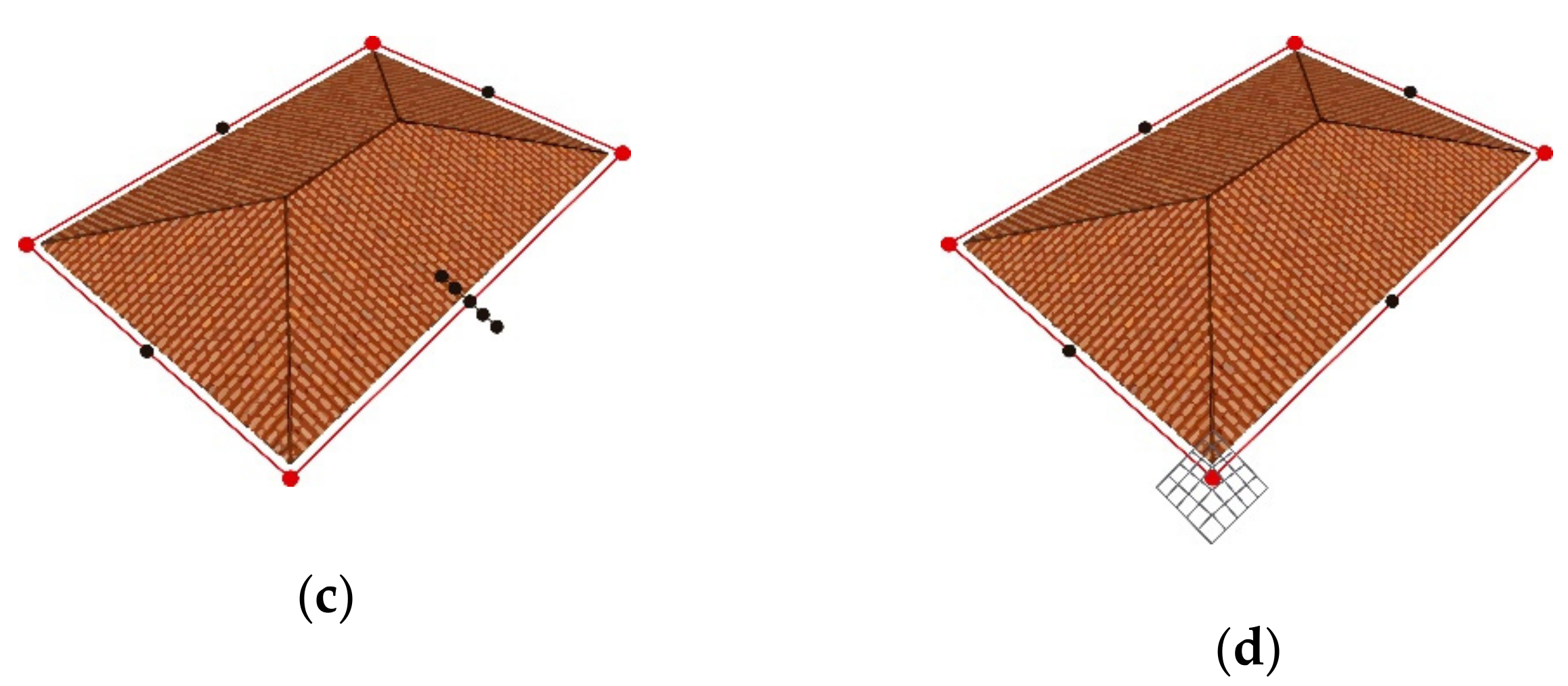
• To begin the extraction process, seed points that approximately describe the boundary should be provided. We use the corner points from the 3D roof model (Figure 7a).
• The 3D polyline is densified inserting midpoints between its points, keeping the existing points (Figure 7b). A separation threshold between the inserted points is used to prevent the excessive densification on small roof sides and maintain a pattern of point density on small and large sides.
• These points—initial and inserted points—are used to create the solution space, which consists of two types of search spaces:

  (a)

  Side search space: is established on the roof side points. It is created by sampling points along straight-line segments simultaneously transversal to the boundary and to the normal vector of the roof plane containing the point under analysis. Hence the straight-line segments generated go along with the roof planes (Figure 7c).

  (b)

  Corner search space: is established on the corner points and is designed by a regular grid in which the points are sampled on the roof plane segment (Figure 7d).

• The DP algorithm is performed considering the solution space created in the previous step in order to determine the 3D polyline that better fits the roof outline. In this step, the auxiliary images of vegetation and shadow, and the visibility map are used to verify if a given point is in any of these regions and establish the appropriate value for each parameter of the Snake energy function. Section 2.3.1 shows how each parameter is set up on the Snake energy function.
• Verify the condition: $∥P^i-P^{i-1}∥<L$, where Pⁱ and Pⁱ⁻¹ are the two last 3D refined polylines, and L is a pre-established threshold. If the condition is not satisfied, return to step 2; otherwise, the optimum polyline Pⁱ was found.

Adaptive Determination of the Energy Function Parameters

This section presents the configuration adopted for each energy function parameter during the optimization process.

Parameter α_i: considering the straight shape of the boundaries, we adopt a unique and high value to α_i, to assign low flexibility to the side segments in order to minimize the influence of points distant from a midline. This property makes the boundaries approach a straight-line.

Parameter β_i: we adopt the null value to β_i at the corner points, to enable the formation of a corner (known as second-order discontinuity). At the other points, that is, side points, β_i has a unique value empirically estimated.

Parameter γ_i: this parameter is related to the external energy term that models the sides’ property. Thus, it has a unique value at the side points and a null value at the corner points (Equation (4)).

Parameter η_i: as opposed to the previous parameter, η_i has a unique value at the corner points and a null value at the side points because it is related to the external energy term that models the corners’ property (Equation (5)).

As presented in Section 2.1, the vegetation image and visibility map allow the method to identify whether a given point is in any obstructed region, making it possible to adapt the parameters of the Snake function (α, β, γ, η) to handle each case. The roof obstruction cases—by high vegetation or viewpoint-dependence—do not affect the Snake’s internal energy, only the external energy. Therefore, γ and η (external energy) must have null value at the obstructed segments, allowing only the internal forces (α and β) to work. The viewpoint-dependent obstructions may appear in only one image of the stereo pair; thus, the external energy force of the non-obstructed image can be used to delineate the roof boundary. On the other hand, the high vegetation obstructions appear in both images of the stereo pair. Consequently, the external energy of both images receives the null value, leaving the control to internal energy forces only.

2.4. Accuracy Assessment Metrics

The assessments are performed based on qualitative and quantitative aspects, comparing the boundaries extracted by the method and the reference boundaries extracted by an operator. In the qualitative assessment, we compare the extracted boundary and the reference boundary superimposed on the aerial image. The quantitative assessment is carried out on the object space based on the metrics of completeness, correctness, and root-mean-square error (RMSE). The completeness and correctness parameters are calculated using the areas of the extracted polylines (A_E) and reference polylines (A_R).

The completeness is related to the omission error and represents the percentage of the reference area that was extracted by the method. The correctness represents the percentage of the extracted area that is correct in relation to the reference area and is related to commission error. The completeness and correctness equations used in this work are presented below [26]:

$$completeness=\frac{A_{E\cap R}}{A_R} 100\%, correctness=\frac{A_{E\cap R}}{A_E} 100\%,$$

(11)

where A_E∩R is the area of intersection between an extracted and a reference polyline, and A_R and A_E are the reference and corresponding extracted polyline areas, respectively. In the experiments section (Section 3), it should be noted that A_E will be the area of the initial polylines when calculating the completeness and correctness of the initial boundaries.

Figure 8 illustrates the concept related to completeness and correctness between two polylines. The polygons filled in red and green represent, respectively, the reference polyline area and the extracted polyline area. The area of intersection between the two is highlighted in magenta. As can be seen, the greater the area of intersection between the polygons, the greater the correspondence between the extracted polyline and the reference polyline.

The RMSE is calculated as a function of the distances between corresponding vertices in the extracted and reference polylines:

$$RMSE=\sqrt{\frac{1}{n}{\displaystyle \sum }_{i=1}^n{d}_i^2},$$

(12)

where d_i is the distance between vertex i of the reference polyline and the corresponding vertex of the extracted polyline, and n is the number of vertices in both polylines.

3. Experimental Results

This section presents the dataset used in this work, the parameters and thresholds used in the experiments, and the experimental results. The results are shown in three different groups, which comprise the situations predicted by the proposed method: roofs obstructed by high vegetation, roofs containing adjacent shadows, and roofs with viewpoint-dependent obstructions. In the last experiment (Section 3.5), there is also a sample that contains all three situations (high vegetation, adjacent shadow, and viewpoint-dependence).

3.1. Dataset

The method assessment was carried out in the urban area of the city of Presidente Prudente, São Paulo state, Brazil. The automatic extraction method proposed in this work plays an important role in the context of urban cadaster update in small Brazilian cities. Since the building information in these cities is manually updated using images or in-situ measurements, making the process costly and time-consuming. As a consequence, many cities in Brazil have flawed urban planning or fail to collect a high amount of taxes because they are unable to keep their urban cadaster up to date. The dataset used to perform the experiments are presented below:

• LiDAR point cloud: was collected from the UNESP Photogrammetric Dataset [31]. The point cloud was acquired by a RIEGL LMS-Q680i Airborne LASER Scanner unit. The average density is 6 points/m². The data was acquired in 2014 with a flight height of 900 m.
• High-resolution aerial images: were collected from the UNESP Photogrammetric Dataset [31]. The camera used was a medium format camera Phase One model iXA 180, based on a CCD (Charge Couple Device) technology and equipped with Schneider-Kreuznach lenses. The nominal focal length was 55 mm, and the image size is 10328 × 7760 pixels. The pixel size is 5.2 × 5.2 micron, and the average ground sample distance (GSD) was 10 cm. The data was acquired in 2014 with a flight height of 900 m.
• Tridimensional roof models: they were created from the LiDAR data. They contain the object-space coordinates of the corner and ridge points, and the plan coefficients.
• Visibility maps: obtained by using Inpho^® software (Trimble). The map has a GSD of 10 cm.

3.2. Parameters

Table 1. Value of the parameters used in the experiments.

Parameters	Value
α	500,000
β	500,000
γ	1
η	500,000
Side search space dimension	9 points
Corner search space dimension	9 × 9 points
Minimal separation between search spaces	1.5 m

shows the values of the parameters used in the boundary extraction procedure. Where α, β, γ, and η are the Snake model parameters; “side search space dimension” and “corner search space dimension” are the dimensions of the search spaces used in the extraction process; and “minimal separation between search spaces” is the threshold to limit the densification of the solution space. It is worth mentioning that all the values were determined by trial and error.

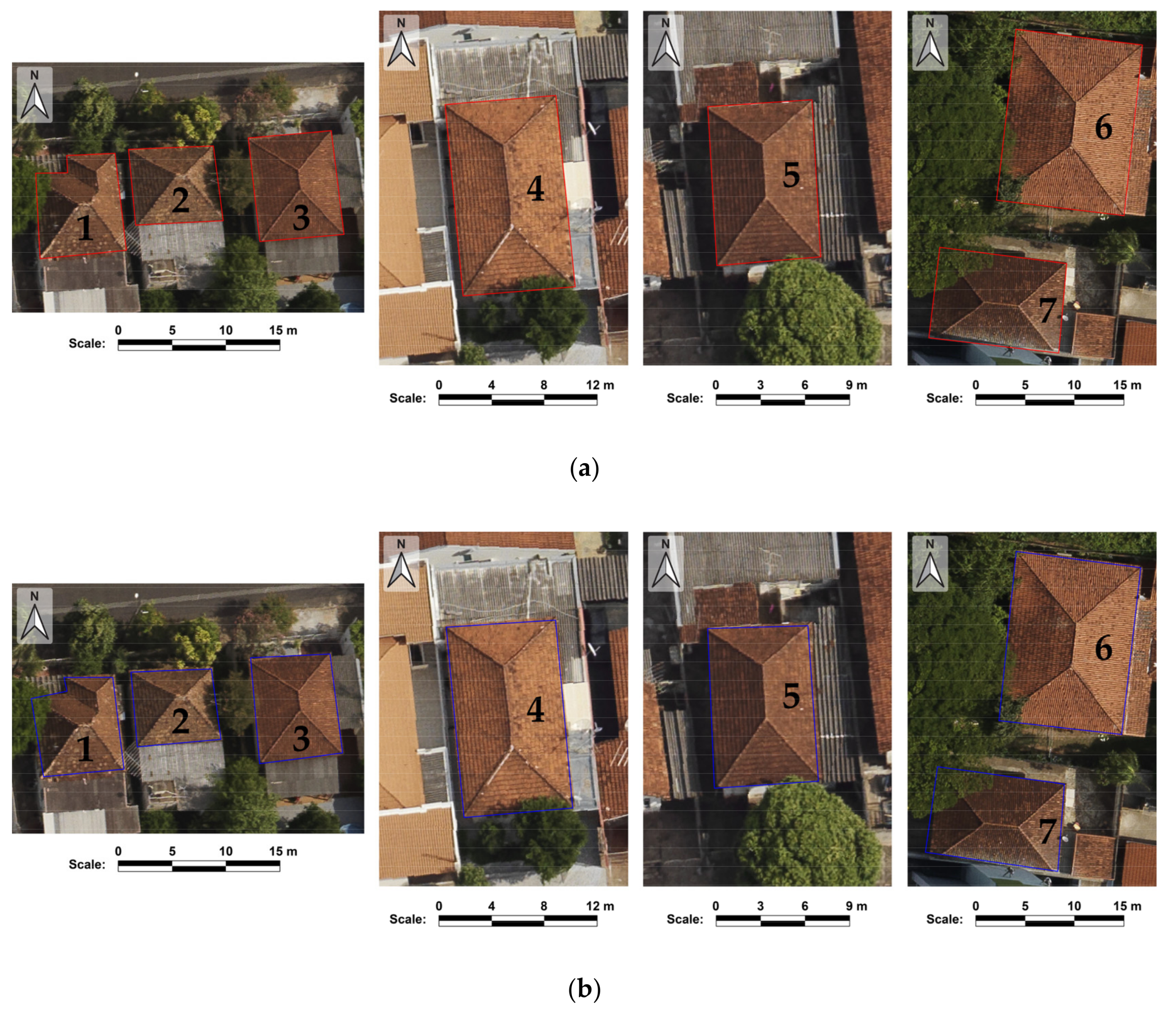
3.3. High Vegetation Obstructions Results

In this experiment, we aimed to test the algorithm performance in cases of high vegetation obstructions. We carried out tests in seven samples, labeled as shown in Figure 9. Figure 9a shows the reference boundary (in red), Figure 9b shows the initial boundary (in blue), and Figure 9c shows the extracted boundary (in green).

It is worth noting that, although the boundaries were extracted in the object space, the projection of them on the image was used to perform the qualitative assessment.

As shown in Figure 9c, the algorithm succeeds in extracting the roof boundaries occluded by vegetation, even though there are no good radiometric responses to model the boundary in these areas. This result could be achieved due to the characteristics of the energy function developed.

On Roof 2 and 3, the occlusions occur on the sides of the roofs, thus, the correct extraction of the contour was favored by term 1 of Equation (7), since by assigning a high value to the parameter α it is possible to force the contour segment to be little flexible, approaching to a straight line.

On Roof 4 and 5, the occlusion appears close to the corner, however, only one side of the corner is obstructed. Thus, the radiometric response of the non-occluded side could be used in term 4 (Equation (7)) to perform the correct extraction in that area.

On Roof 1, 6, and 7, the occlusions occur in corner regions. In this case, the angular component ($1-\cos \left({\delta }_i\right)$) of term 4 of Equation (7) favored the right-angled corners, enabling the correct extraction in these regions.

Table 2. Quality parameters of the high vegetation obstructions experiment.

	Roof	Completeness (%)	Correctness (%)	RMSEE (m)	RMSEN (m)	RMSEH (m)
Initial boundaries	1	89.69	99.67	0.27	0.35	0.75
	2	83.65	100.00	0.29	0.39	0.69
	3	88.76	97.02	0.41	0.27	0.60
	4	92.35	96.99	0.33	0.46	1.25
	5	89.14	98.95	0.36	0.28	1.13
	6	96.25	98.86	0.21	0.21	0.38
	7	96.25	93.31	0.35	0.30	0.95
	Average	90.87	97.83	0.32	0.32	0.82
Extracted boundaries	1	95.86	92.18	0.30	0.22	0.61
	2	94.51	96.49	0.23	0.16	0.54
	3	99.23	95.68	0.22	0.28	0.52
	4	97.42	94.69	0.27	0.25	1.14
	5	96.66	93.24	0.34	0.21	0.94
	6	98.29	98.19	0.11	0.23	0.34
	7	96.20	98.39	0.22	0.18	0.91
	Average	96.88	95.55	0.24	0.22	0.71

summarizes the accuracy assessment result of initial boundaries and extracted boundaries in all samples. The third column shows the resulting completeness values, the fourth column shows the resulting correctness values, and the three last columns present the resulting geometrical accuracy in E, N, and H components.

It can be noted that the average completeness value of the extracted boundaries (96.88%) was greater than the initial boundaries (90.87%), which indicates the boundaries’ enhancement when using the proposed method. Furthermore, the average RMSE_E,N values improved from 0.32 m (initial boundaries) to 0.24 m/0.22 m (extracted boundaries), and the average RMSE_H value improved from 0.82 m (initial boundaries) to 0.71 m (extracted boundaries), proving over again the method efficiency.

3.4. Adjacent Shadow Results

In this second experiment, the tests aimed to demonstrate the proposed method’s effectiveness on roofs with adjacent shadows, which could be misinterpreted as roof edges. The selected test area contains five roofs with adjacent shadows, labeled as shown in Figure 10. On Roof 5, in addition to the shadow, there is also a high vegetation occlusion. Figure 10a shows the reference boundary (in red), Figure 10b shows the initial boundary (in blue), and Figure 10c shows the extracted boundary (in green).

As can be seen from Figure 10c, the proposed algorithm correctly extracted the edges with adjacent shadows in all roofs. In theory, the shadow edges will produce higher energy to the Snake function because the gradient responses are higher in those areas when compared to the roof edges. However, the shadow compensation factor introduced in term 3 of Equation (7) was able to analyze which points belong to the roof edge and which points belong to the shadow edge, thus supporting the correct choice of the roof edge points. Furthermore, the edge obstructed by the vegetation on Roof 5 also was adequately extracted.

In some cases, such as on Roof 1 (detailed in Figure 10c), it is possible to note a small deviation in the detected boundary caused by features around the roofs, which confuse and impair the correct detection of the boundary. In this case, a pre-processing of the image, such as by segmentation, could minimize this type of problem.

Table 3. Quality parameters of the adjacent shadow experiment.

	Roof	Completeness (%)	Correctness (%)	RMSEE (m)	RMSEN (m)	RMSEH (m)
Initial boundaries	1	92.50	99.97	0.23	0.29	0.51
	2	89.73	100.00	0.34	0.30	0.35
	3	93.28	100.00	0.22	0.26	0.64
	4	87.08	100.00	0.37	0.35	0.40
	5	87.67	100.00	0.28	0.35	0.48
	Average	90.05	99.99	0.29	0.31	0.48
Extracted boundaries	1	99.91	97.37	0.13	0.09	0.43
	2	99.75	98.75	0.04	0.12	0.22
	3	99.72	97.04	0.15	0.12	0.53
	4	98.13	97.70	0.12	0.10	0.28
	5	99.09	96.92	0.16	0.14	0.36
	Average	99.32	97.56	0.12	0.11	0.36

presents the accuracy assessment result of the initial boundaries and the extracted boundaries. The average completeness value of the extracted boundaries (99.32%) was greater than the initial boundaries (90.05%), indicating the correct boundaries refinement. Regarding the initial boundary correctness, almost all the roofs obtained a value of 100%. These values stem from the fact that all initial boundaries are inside the reference boundaries. As mentioned before, the correctness parameter shows how much the analyzed area is correct in relation to the reference area. Consequently, if the entire analyzed area—in this case, the area of the initial polylines—is inside the reference area, the entire analyzed area will be correct and its correctness will be 100%.

The average values of RMSE_E,N improved from 0.30 m (initial boundaries) to 0.10 m (extracted boundaries), approximately. Whereas the average values of RMSE_H improved from 0.48 m (initial boundaries) to 0.36 m (extracted boundaries).

3.5. Viewpoint-Dependent Obstructions Results

The last experiment aimed to assess the proposed method’s performance in viewpoint-dependent obstructions cases (occlusion areas). To take advantage of using the stereo pair of images, we selected situations where the obstructions appear in only one of the images. It is worth noting that if the occlusion appears in both images, another image could be used to establish a new stereo pair. Figure 11 shows the stereo pair of images used in this experiment.

Figure 12a–c present the reference boundary (in red), the initial boundary (in blue), and the extracted boundary (in green), respectively. It can be noted that the method succeeds in delineating the boundaries accurately on the obstructed regions. This is because in these regions, the region obstructed in one of the images, the non-obstructed image response was used to calculate the energy function leading to a correct result.

On Roof 1, we have a complete experiment with all three scenarios—viewpoint-dependent obstruction, high vegetation obstruction and adjacent shadow. As demonstrated in Section 3.3 and Section 3.4, the proposed method works efficiently in these situations. However, one can remark in Figure 13 that the white feature on one of the edges (circled in magenta in Figure 12c) caused the wrong delineation of the correct edge (magenta dashed line in Figure 13). This result shows the method’s sensitivity to noise close to the edges, making it interesting to perform a pre-processing of the image to eliminate these noises before applying the boundary extraction method.

Table 4. Quality parameters of the viewpoint-dependent obstruction experiment.

	Roof	Completeness (%)	Correctness (%)	RMSEE (m)	RMSEN (m)	RMSEH (m)
Initial boundaries	1	93.50	95.50	0.42	0.33	0.93
	2	93.01	97.73	0.28	0.29	1.46
	Average	93.26	96.62	0.35	0.31	1.20
Extracted boundaries	1	94.46	97.96	0.31	0.28	0.91
	2	97.86	94.83	0.29	0.27	1.34
	Average	96.16	96.40	0.30	0.28	1.13

shows the accuracy assessment result of the initial boundaries and the extracted boundaries. Once again, the average completeness value of the extracted boundaries (96.16%) was better than the initial boundaries (93.26%). Concerning the RMSE values, the improvement between the initial boundaries and the extracted boundaries was only marginal.

4. Discussion

4.1. Performance

The qualitative assessment (Figure 9, Figure 10 and Figure 12) of the results showed that the proposed method can delineate the roof boundary even in obstruction scenario and adjacent shadow anomalies. However, it can be noted that some boundaries were affected by noises around the roof edges. It can also be noted that the new approach proposed for calculating the corner response can delineate right-angled corners, avoiding the problem of extracted boundaries slightly “rounded” around the building corners, which is present in several works involving the Snake model. However, in some experiments, the location of the extracted corner was not the correct location of the corner.

In the high vegetation obstruction experiments (Figure 9), the geometric terms (internal forces) of the Snake-based model were used to guide the boundary extraction. If the obstruction is in a side region, the parameter γ will receive a null value since there will be no radiometric response. Thus, the task of delineating the obstructed boundary will be controlled by the internal force parameter α. By assigning a high value to the parameter α, we can minimize the influence of points distant from a midline, making the boundaries approach a straight-line. If the obstruction is in a corner region, the parameter η will receive the null value since there will be no radiometric response. Thus, the step of delineating the obstructed corner will be controlled by the internal force β. Adopting the null value to β enable the formation of a corner (known as second-order discontinuity). In the adjacent shadow experiments (Figure 10), the shadow compensation factor introduced in the Snake-based model was able to distinguish which points belong to the roof edge and which points belong to the shadow edge. In the viewpoint-dependent obstructions experiments (Figure 12), the non-obstructed image provided the necessary boundary information for the delineation. In addition, despite the increase of data to process, the processing time of the algorithm is not affected due to the optimization method used — Dynamic Programming.

From the quantitative assessment (Table 2, Table 3, Table 4) it can be seen that the extracted boundaries provided better values than the initial boundaries. The RMSE_E,N,H had an improvement around 0.10 m–0.20 m. The completeness parameter improved from an average of 90 to 96–99%. On the other hand, the initial boundaries had higher correctness values than the extracted boundaries. As explained in Section 3.4, this is because the initial boundaries were inside the reference boundaries.

4.2. Limitations

Although the good outcomes, there are some limitations in the proposed method that are worth deepening in future work. The experiments showed that the method is sensitive to noises, i.e., the boundary detection is affected by objects and features around the roofs. These results show that a pre-processing of the image using a suitable segmentation method would improve the boundary delineation. Regarding the Snake-based model, the automatic definition of its parameters was not a goal of this work, but it is a significant subject to be studied since the determination by trial and error is time-consuming and operator-dependent.

As presented before, the method can avoid the problem of extracted boundaries slightly “rounded” around the building corners, but the location of the extracted corner is often not the correct location. This result indicates the need for a process to refine the position of the detected corner. Furthermore, the method covers only right-angled roofs, so it can not work with other types of roofs, such as curved roofs.

The extraction method can work on roofs with few obstructed areas. However, on buildings with a high percentage of obstruction (e.g., more than 50%), the method may not be effective, since there will not be enough geometric information to guide the correct delineation.

Another limitation faced by the method is the fact that the shadow compensation factor is totally dependent on the shadow image, i.e., the compensation factor will only be applied to a shadow region if this region is detected in the shadow image. Otherwise, the extraction process will not consider the shadow region, which may provide an incorrect result.

Despite all the advantages of using the stereo pair, the scenario suggested by this work—occlusion in only one of the stereo pair images—is not so easy to be found, since it depends on several factors such as height and direction of the flight, height of the building that causes the occlusion, the position of the perspective center, terrain displacement, etc. Thus, if the occlusion appears in both images, the problem becomes a case of simple occlusion and can be solved using a single image. Another solution would be to use a true-orthophoto.

One more aspect that should be included in further discussion is the behavior of the method in sustainable building areas, such as the ones with green roofs. This characteristic could mislead the algorithm to a bad roof boundary extraction. However, considering that these buildings usually do not have an irregular type of vegetation—they are small and continuous—its classification could be handled by changing the planarity and roughness parameters in the LiDAR classification process.

5. Conclusions

In this paper, we presented an automatic method to extract roof boundaries directly in object space by integrating a stereo pair of images and 3D roof models obtained from LiDAR data. The roof boundaries do not have a good definition in low-density LiDAR data, making interesting the integration with image data to improve the edge positional accuracy, since the edges are well defined in optical images. On the other hand, the 3D roof models can provide altimetric information about the edge points. Therefore, the integration of these two data sources proposed by this work proved to be a solution to extract the roof boundaries directly in the object space.

This work also proposed a solution to typical problems related to roof boundary extraction in the urban environment: obstruction caused by high vegetation covering part of the roof; shadows adjacent to the roofs, which can be misinterpreted as roof edges; and roof viewpoint-dependent obstructions caused by high neighboring buildings (occlusions). To overcome these situations, an improved Snake model (Equation (7)) was developed incorporating terms that enable the correct detection of the roof boundary, even in the presence of the problems mentioned above. Furthermore, the created Snake-based model presents a new approach for calculating the corner response, combining the radiometric and geometric information of the candidate points to the corner.

These findings show that the inclusion of the new approaches presented in this work contributes to the development of the state-of-the-art involving the roof boundaries extraction, reducing the problems encountered by other authors. These advances also provide the improvement of 3D building and city models. Therefore, we can mention some fields in which the technology presented in this work can be useful. The Smart City is a subject that has been growing in the last years. The concept of Smart City is to optimize the efficiency of city services by integrating spatial data, policy and governance, data sharing platforms, and applications, services, and solutions. According to Jovanovic et al. [32], one of the main areas of application of the 3D city models for Smart Cities is the modeling and simulations involving impact on the environment, such as energy efficiency of urban areas, urban building energy modeling, city-wide energy simulations, solar energy resources in cities, urban energy simulation for climate protection, disaster management, and homeland security.

References

1. Chen, J.; Dowman, I.; Li, S.; Li, Z.; Madden, M.; Mills, J.; Paparoditis, N.; Rottensteiner, F.; Sester, M.; Toth, C.; et al. Information from imagery: ISPRS scientific vision and research agenda. ISPRS J. Photogramm. Remote Sens. 2016, 115, 3–21. [Google Scholar] [CrossRef] [Green Version]
2. Benciolini, B.; Ruggiero, V.; Vitti, A.; Zanetti, M. Roof planes detection via a second-order variational model. ISPRS J. Photogramm. Remote Sens. 2018, 138, 101–120. [Google Scholar] [CrossRef]
3. Huang, J.; Zhang, X.; Xin, Q.; Sun, Y.; Zhang, P. Automatic building extraction from high-resolution aerial images and LiDAR data using gated residual refinement network. ISPRS J. Photogramm. Remote Sens. 2019, 151, 91–105. [Google Scholar] [CrossRef]
4. Ghanea, M.; Moallem, P.; Momeni, M. Building extraction from high-resolution satellite images in urban areas: Recent methods and strategies against significant challenges. Int. J. Remote Sens. 2016, 37, 5234–5248. [Google Scholar] [CrossRef]
5. Alshehhi, R.; Marpu, P.R.; Woon, W.L.; Mura, M.D. Simultaneous extraction of roads and buildings in remote sensing imagery with convolutional neural networks. ISPRS J. Photogramm. Remote Sens. 2017, 130, 139–149. [Google Scholar] [CrossRef]
6. Xu, Y.; Wu, L.; Xie, Z.; Chen, Z. Building extraction in very high resolution remote sensing imagery using deep learning and guided filters. Remote Sens. 2018, 10, 144. [Google Scholar] [CrossRef] [Green Version]
7. Wu, G.; Shao, X.; Guo, Z.; Chen, Q.; Yuan, W.; Shi, X.; Xu, Y.; Shibasaki, R. Automatic building segmentation of aerial imagery using multi-constraint fully convolutional networks. Remote Sens. 2018, 10, 407. [Google Scholar] [CrossRef] [Green Version]
8. Nguyen, T.H.; Daniel, S.; Guériot, D.; Sintès, C.; Le Caillec, J.-M. Super-resolution-based Snake model—An unsupervised method for large-scale building extraction using airborne LiDAR data and optical image. Remote Sens. 2020, 12, 1702. [Google Scholar] [CrossRef]
9. Yang, B.; Xu, W.; Dong, Z. Automated extraction of building outlines from airborne laser scanning point clouds. IEEE Geosci. Remote Sens. Lett. 2013, 10, 1399–1403. [Google Scholar] [CrossRef]
10. Tomljenovic, I.; Höfle, B.; Tiede, D.; Blaschke, T. Building extraction from airborne laser scanning data: An analysis of the state of the art. Remote Sens. 2015, 7, 3826–3862. [Google Scholar] [CrossRef] [Green Version]
11. Du, S.; Zhang, Y.; Zou, Z.; Xu, S.; He, X.; Chen, S. Automatic building extraction from LiDAR data fusion of point and grid-based features. ISPRS J. Photogramm. Remote Sens. 2017, 130, 294–307. [Google Scholar] [CrossRef]
12. Pirasteh, S.; Rashidi, P.; Rastiveis, H.; Huang, S.; Zhu, Q.; Liu, G.; Li, Y.; Li, J.; Seydipour, E. Developing an algorithm for buildings extraction and determining changes from airborne LiDAR, and comparing with R-CNN method from drone images. Remote Sens. 2019, 11, 1272. [Google Scholar] [CrossRef] [Green Version]
13. Zarea, A.; Mohammadzadeh, A. A novel building and tree detection method from LiDAR data and aerial images. IEEE J. Sel. Top. Appl. Earth Obs. Remote Sens. 2016, 9, 1864–1875. [Google Scholar] [CrossRef]
14. Gilani, S.A.N.; Awrangjeb, M.; Lu, G. An automatic building extraction and regularisation technique using LiDAR point cloud data and orthoimage. Remote Sens. 2016, 8, 258. [Google Scholar] [CrossRef] [Green Version]
15. Lari, Z.; El-Sheimy, N.; Habib, A. A new approach for realistic 3D reconstruction of planar surfaces from laser scanning data and imagery collected onboard modern low-cost aerial mapping systems. Remote Sens. 2017, 9, 212. [Google Scholar] [CrossRef] [Green Version]
16. Fernandes, V.J.M.; Dal Poz, A.P. Extraction of building roof contours from the integration of high-resolution aerial imagery and laser data using Markov random fields. Int. J. Image Data Fusion 2018, 9, 263–286. [Google Scholar] [CrossRef]
17. Chen, Q.; Wang, S.; Liu, X. An improved Snake model for refinement of LiDAR-derived building roof contours using aerial images. Int. Arch. Photogramm. Remote Sens. Spat. Inf. Sci. 2016, XLI-B3, 583–589. [Google Scholar] [CrossRef] [Green Version]
18. Sun, Y.; Zhang, X.; Zhao, X.; Xin, Q. Extracting building boundaries from high resolution optical images and LiDAR data by integrating the convolutional neural network and the active contour model. Remote Sens. 2018, 10, 1459. [Google Scholar] [CrossRef] [Green Version]
19. Griffiths, D.; Boehm, J. Improving public data for building segmentation from Convolutional Neural Networks (CNNs) for fused airborne LIDAR and image data using active contours. ISPRS J. Photogramm. Remote Sens. 2019, 154, 70–83. [Google Scholar] [CrossRef]
20. Oliveira, H.C.; Dal Poz, A.P.; Galo, M.; Habib, A.F. Surface gradient approach for occlusion detection based on triangulated irregular network for true orthophoto generation. IEEE J. Sel. Top. Appl. Earth Obs. Remote Sens. 2018, 11, 443–457. [Google Scholar] [CrossRef]
21. Azevedo, S.C.; Sival, E.A.; Pedrosa, M.M. Shadow detection improvement using spectral indices and morphological operators in urban areas in high resolution images. Int. Arch. Photogramm. Remote Sens. Spat. Inf. Sci. 2015, XL-7/W3, 587–592. [Google Scholar] [CrossRef] [Green Version]
22. Soille, P. Morphological Image Analysis; Springer: Berlin, Germany, 2004. [Google Scholar]
23. Otsu, N. A threshold Selection Method from Gray-Level Histograms. IEEE Trans. Syst. Man Cybern. 1979, 9, 62–69. [Google Scholar] [CrossRef] [Green Version]
24. Axelsson, P. Processing of laser scanner data: Algorithms and applications. ISPRS J. Photogramm. Remote Sens. 1999, 54, 138–147. [Google Scholar] [CrossRef]
25. Wolf, P.R.; Dewitt, B.A. Elements of Photogrammetry–with Applications in GIS, 3rd ed.; McGraw-Hill: New York, NY, USA, 2000. [Google Scholar]
26. Mikhail, E.M.; Bethel, J.S.; McGlone, J.C. Introduction to Modern Photogrammetry; John Wiley & Sons: New York, NY, USA, 2001. [Google Scholar]
27. Kass, M.; Witkin, A.; Terzopoulous, D. Snakes: Active contour models. Int. J. Comput. Vis. 1988, 1, 321–331. [Google Scholar] [CrossRef]
28. Fazan, A.J.; Dal Poz, A.P. Rectilinear building roof contour extraction based on snakes and dynamic programming. Int. J. Appl. Earth Obs. Geoinf. 2013, 25, 1–10. [Google Scholar] [CrossRef]
29. Moravec, H.P. Towards automatic visual obstacle avoidance. In Proceedings of the 5th International Joint Conference on Artificial Intelligence, Cambridge, MA, USA, 22–25 August 1977. [Google Scholar]
30. Ballard, D.; Brown, C.M. Computer Vision; Prentice Hall: Hoboken, NJ, USA, 1982. [Google Scholar]
31. Tommaselli, A.M.G.; Galo, M.; Dos Reis, T.T.; Ruy, R.S.; De Moraes, M.V.A.; Matricardi, W.V. Development and assessment of a dataset containing frame images and dense airborne laser scanning point clouds. IEEE Geosci. Remote Sens. Lett. 2018, 15, 192–196. [Google Scholar] [CrossRef]
32. Jovanovic, D.; Milovanov, S.; Ruskovski, I.; Govedarica, M.; Sladic, D.; Radulovic, A.; Pajic, V. Building virtual 3D city model for Smart Cities applications: A case study on campus area of the University of Novi Sad. ISPRS Int. J. Geo Inf. 2020, 9, 476. [Google Scholar] [CrossRef]
Figure 1. Flowchart of the proposed method.
Remotesensing 13 01429 g001
Figure 2. (a) Sample of the visibility map, where the blue area is the occluded region. (b) Corresponding aerial image.
Remotesensing 13 01429 g002
Figure 3. Example of shadow regions detection. (a) Details of a high-resolution aerial image. (b) Detected shadows (in white) in the original image. (c) Detected shadows (in white) in the smoothed image. (d) Final shadow image.
Remotesensing 13 01429 g003
Figure 4. LiDAR point cloud classification steps. (a) Aerial image of the region. (b) Ground (magenta) and non-ground (yellow) points. (c) Building (red) and vegetation (green) points. (d) Vegetation points (white) projected onto the image space. (e) Vegetation image based on the morphological operator.
Remotesensing 13 01429 g004
Figure 5. Shadow compensation factor. (a) Gradient vector at the roof edge point and the vector pointing at the roof’s barycenter. (b) Gradient vector at the shadow edge point and vector that points to the roof’s barycenter.
Remotesensing 13 01429 g005
Figure 6. Elements for defining the term CS for the calculation of the corner response.
Remotesensing 13 01429 g006
Figure 7. The creation of the 3D solution space. (a) Initial boundary. (b) Densified boundary in the first iteration. (c) Side search space. (d) Corner search space.
Remotesensing 13 01429 g007aRemotesensing 13 01429 g007b
Figure 8. Illustration of the completeness and correctness between two polylines.
Remotesensing 13 01429 g008
Figure 9. High vegetation obstruction samples. (a) Reference boundaries (red). (b) Initial boundaries (blue). (c) Extracted boundaries (green).
Remotesensing 13 01429 g009aRemotesensing 13 01429 g009b
Figure 10. Adjacent shadows samples. (a) Reference boundaries (red). (b) Initial boundaries (blue). (c) Extracted boundaries (green).
Remotesensing 13 01429 g010
Figure 11. Viewpoint-dependent obstruction samples.
Remotesensing 13 01429 g011
Figure 12. Visual results of the viewpoint-dependent obstruction experiment. (a) Reference boundaries (red). (b) Initial boundaries (blue). (c) Extracted boundaries (green).
Remotesensing 13 01429 g012
Figure 13. Incorrect boundary extraction caused by the white feature on the edge, extracted boundary (green), and correct boundary (dashed magenta).
Remotesensing 13 01429 g013