A Low-Cost and Robust Landsat-Based Approach to Study Forest Degradation and Carbon Emissions from Selective Logging in the Venezuelan Amazon

Abstract

Selective logging in the tropics is a major driver of forest degradation by altering forest structure and function, including significant losses of aboveground carbon. In this study, we used a 30-year Landsat time series (1985–2015) to analyze forest degradation and carbon emissions due to selective logging in a Forest Reserve of the Venezuelan Amazon. Our work was conducted in two phases: the first, by means of a direct method we detected the infrastructure related to logging at the sub-pixel level, and for the second, we used an indirect approach using buffer areas applied to the results of the selective logging mapping. Pre- and post-logging forest inventory data, combined with the mapping analysis were used to quantify the effects of logging on aboveground carbon emissions for three different sources: hauling, skidding and tree felling. With an overall precision of 0.943, we demonstrate the potential of this method to efficiently map selective logging and forest degradation with commission and omission errors of +7.6 ± 4.5 (Mean ± SD %) and −7.5% ± 9.1 respectively. Forest degradation due to logging directly affected close to 24,480 ha, or about ~1% of the total area of the Imataca Forest Reserve. On average, with a relatively low harvest intensity of 2.8 ± 1.2 trees ha⁻¹ or 10.5 ± 4.6 m³ ha⁻¹, selective logging was responsible for the emission of 61 ± 21.9 Mg C ha⁻¹. Lack of reduced impact logging guidelines contributed to pervasive effects reflected in a mean reduction of ~35% of the aboveground carbon compared to unlogged stands. This research contributes to further improve our understanding of the relationships between selective logging and forest degradation in tropical managed forests and serves as input for the potential implementation of projects for reducing emissions from deforestation and forest degradation (REDD+).

1. Introduction

More than 400 million hectares (ha) of natural tropical forests have been designated as production forests globally [1,2,3]. Moreover, about 40% of sawn wood traded annually in tropical regions has an origin in natural forests [4], often under a “selective logging” approach in which large trees of a relatively low number of tree species are harvested in rotation cycles of 30 years on average [2,5,6]. With some exceptions, one of the main features of selective logging across the tropics has been the insufficient adoption of reduced impact methods with negative environmental effects on forest structure and function [7,8].

Forest degradation is a change process caused by anthropogenic and/or environmental forces that result in alterations within any given forest, negatively affecting the structure and or function of the stand and site, and thereby lowering the capacity to sustain a continuous supply of products and/or services [9]. Selective logging, a major degradation driver in tropical forests, may account for at least half of the total carbon emissions coming from tropical forest degradation, representing ~6% of total tropical greenhouse gas emissions [10,11]. Logging can cause significant losses in the aboveground carbon in tropical forests up to 10–50% [12,13], and in some cases can add up to 123% more forest-area damage above what has been reported for deforestation alone [14]. Moreover, in tropical regions of Latin America and Asia, selective logging has been responsible for more than 70% of the area of total forest degradation [15], and is often consider a preamble to deforestation processes [16,17,18]. Consequently, in recent years, forest degradation has become a major topic of discussion within the international scientific community as a factor of great importance in the global carbon cycle [11,19,20]. This process has been addressed in the United Nations Framework Convention on Climate Change (UNFCCC) since the Bali agreement in 2007 (CP. 13), when the concept of reducing emissions from deforestation (RED) was expanded to REDD+ to include forest management activities [21], and currently with the so called Nationally Determined Contributions to the UN Paris Climate Agreement [22].

Venezuela has a long history of natural forest management under long-term concession contracts that started in the early 1970s [23,24]. By 1992, almost 3.2 million ha were allocated to more than 30 forest management units (FMUs) and had management plans approved by the national government [25]. However, a remarkable decline in the use of forests as reliable sources of timber has been evident in the last 30 years. According to the last available official data from 2018, only about 2.5% of the wood legally consumed in the country came from FMUs in an estimated area of 246,313 ha of forests with formal management plans mostly in the Amazon region of the country [26].

Forests in the Venezuelan Amazon account for at least 83% of the national forest cover [27]. In this region, forests have been managed via various legal protection schemes, from strictly protected areas such as national parks to others with sustainable use objectives as the case of forest reserves, forest lots and forest areas under protection [28,29]. One of the most important reserves in the region is the Imataca Forest Reserve (IFR), which harbor important levels of biodiversity [30]. In addition, different studies have estimated that the region represents one of the most carbon-rich areas in Venezuela with an average of 205 ± 15 Mg C ha⁻¹ in the aboveground biomass (AGB) [31,32]. At the same time, the IFR is considered a hot spot of deforestation [33] and was recently labelled as one of the deforestation fronts of the tropical belt [34]. In the last two decades, approximately 1144 ha of forests have been lost every year due to mining activities (55.5%), land use change for livestock (26.5%) and agriculture expansion (17.9%) [35]. Yet, from the close to 4 million ha that IFR covers, about 97% is still covered by different forest-types, mostly dominated by lowland “terra firme” forests [35].

Selective logging, via legal, yet mostly unplanned conventional timber harvesting operations was formally authorized in IFR around the 1980’s decade and has become a major factor of anthropogenic disturbance since then [35]. In a standard logging operation in this region, large trees with diameters at breast height (dbh) > 40 cm and with an average height between 20−30 m from a few commercially valuable species are harvested, where for every tree harvested close to 11 additional trees can be severely affected [36]. Moreover, without adequate planning, the impacts of these operations can double the background rates of tree mortality when compared to unlogged stands while also causing a significant reduction in aboveground carbon [13].

To quantify carbon emissions caused by forest degradation as a result of selective logging, two analytical techniques can be used: the first combines logging rates, management plans, and high-resolution imagery for activity data (AD) and the gain/loss approach for emission factors (EFs) [10,37]. The second combines remote detection of medium-resolution images for AD and an assessment of the changes in carbon stocks for EFs [38,39]. For the second technique, the AD can be obtained by a direct method, identifying and mapping canopy damage [40,41,42,43,44,45], or by mapping canopy damage in combination with intact forests and regeneration patches [46,47]. Using an indirect method that implies identifying selective logging in the images, and the addition of buffer areas via geographic information system (GIS) tools, the area of degraded forests due to logging can be quantified [18,48,49]. With this method, the intact forest concept and evaluation criteria are applied to categorize intact and non-intact forests, which discriminate against forests with different carbon stocks [16,46]. The EFs can then be obtained using data collected from field inventories measured before and after logging, with the general change in the carbon reserves calculated using the difference between these two measurements [39].

In this study, we propose an analytical approach based on a Landsat time series [40,41,50,51], developed for the Monitoring System of Deforestation of the Amazon (TerraAmazon) [52]. One of the main goals of our approach is to produce a local-based computing analytical approach capable of functioning under conditions of limited connectivity. We believe this to be an important advantage to conduct an assessment of forest degradation produced by logging in Venezuela’s Imataca Forest Reserve (IFR) for a 30-year period between 1985 and 2015 under different conditions. Overall, because of the general lack of reduced impact logging guidelines being applied [29], we expected that despite a relatively low logging intensity typically between 10 to 12 m³ ha⁻¹ [36,53,54], compared to an average of 20 m³ ha⁻¹ for the Amazon [55], carbon losses could be significant. We put our results in the context of other studies where the effects of logging on carbon have been addressed.

2. Materials and Methods

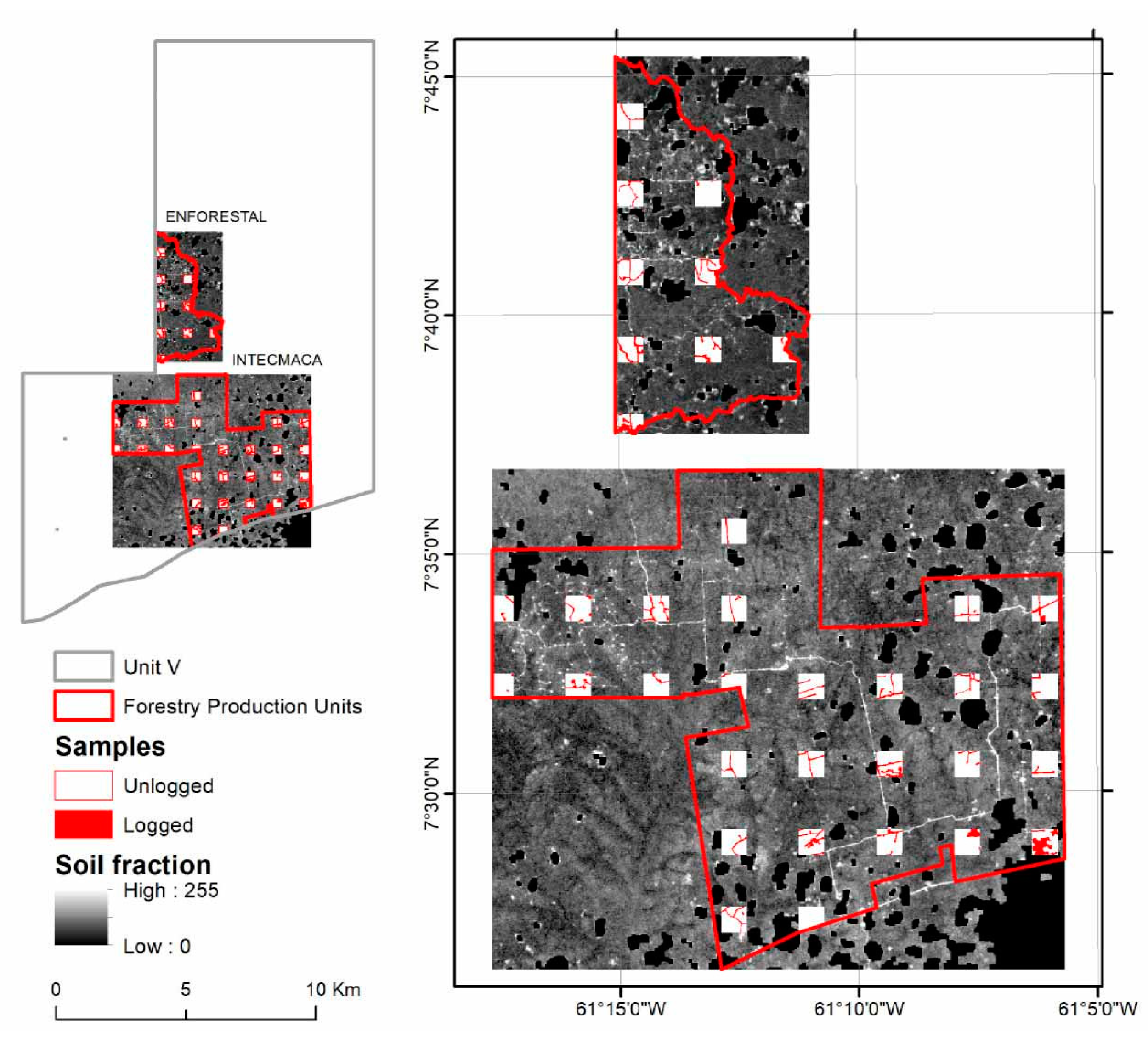
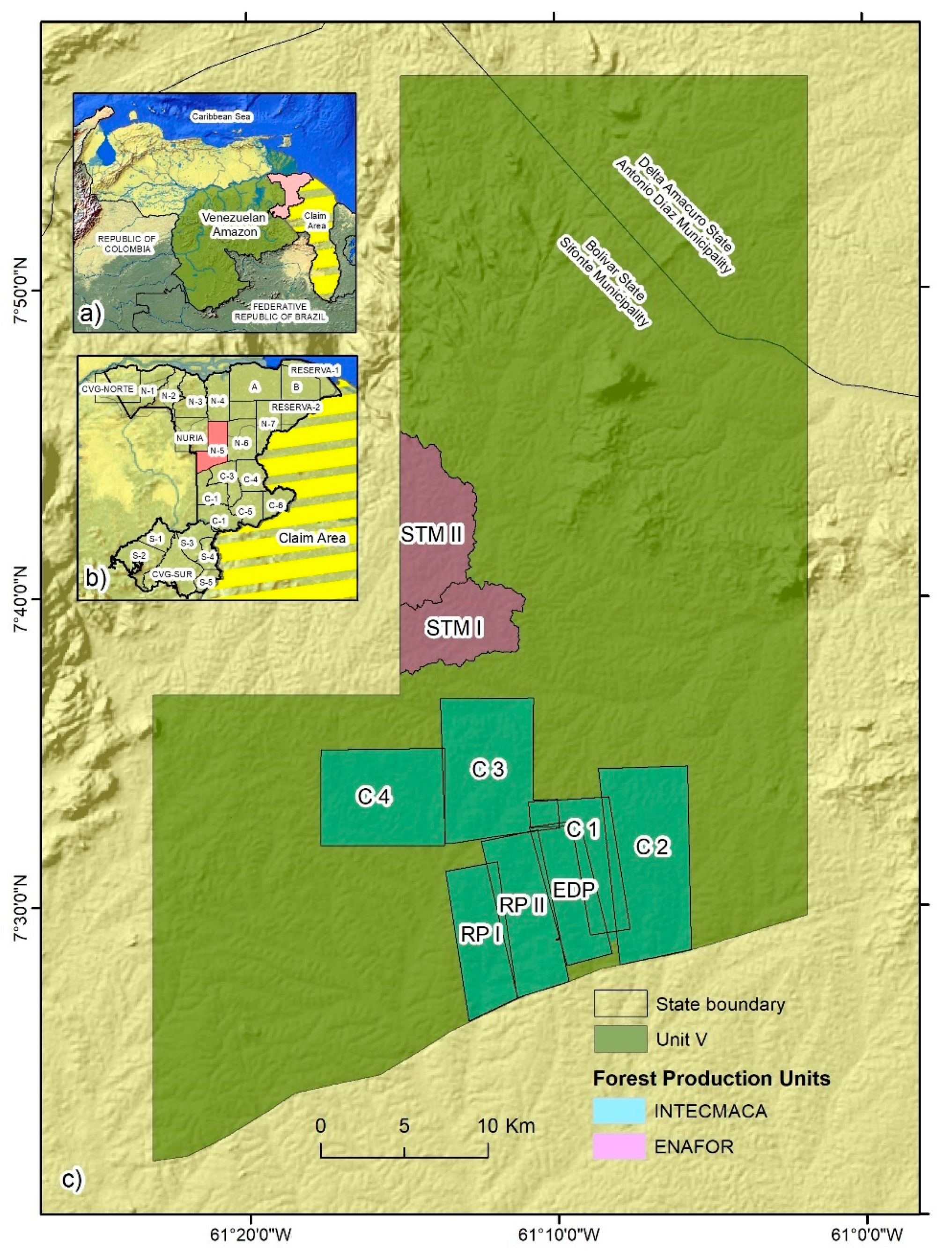
2.1. Study Area

Imataca Forest Reserve (IFR), located in southeastern Venezuela between Bolívar and Delta Amacuro states, was officially created in 1961 and has a total area of 3,821,900 ha, which represents 8.1% of the total area of the Venezuelan Amazon (~46.9 M ha) (Figure 1a). The reserve has been divided into 23 different management units distributed across three major zones (north, central, and south) (Figure 1b). 90% of these units with extensions between 120,000 and 340,000 ha have been designated for permanent forest production, while the rest is officially allocated for mining activities and/or conservation of biodiversity. Between 1985 and 2012, about half of the timber-production areas at IFR was managed under a private concession model where national government granted management rights after an official management plan was approved with cutting cycles ranging from 25 to 40 years [29]. In recent years, with the enactment of the Forests and Forest Management Law of 2008, a policy shift began with regards to how forest management should be planned and applied in Venezuela. Along with government agencies and the newly created National Forest Company (ENAFOR), guidelines for developing new forest management plans were put in place to gradually shift from the model of private concessions to a more government-dominated approach. At present, the company supervises the management for all production forests in the country and is directly responsible for an active management operation in the Imataca Forest Reserve.

The IFR has a northeast-southwest pattern in the distribution of precipitation from 1000 mm to 3000 mm per year approximately. The average annual temperature is around 25 and 27 °C, evapotranspiration ranges from 1250 mm to 1400 mm per year. Overall, in this area we find lowland tropical humid forests, seasonal evergreen forests, deciduous forests and swamp forests. From the standpoint of species diversity around 2800 species of plants, 450 species of birds, 153 species of mammals, 90 species of reptiles, 62 species of amphibians and 242 species of fish have been identified [30].

The management Unit V located in the central region of IFR was selected as a study case. The unit has a total area of 180,000 ha and was first granted management rights to the company Industria Técnica de Maderas C.A (INTECMACA) in 1982. The unit was originally divided into 25 logging compartments of an approximate equal area each according to a 25-year cutting cycle. One component of our work is based on pre- and post-logging inventories conducted at seven of these compartments namely: research plot I (RP I), research plot II (RP II), experimental development plot (EDP), compartment 1 (C1), compartment 2 (C2), compartment 3 (C3) and compartment 4 (C4). After operations were halted by the end of 1990’s, the management was later transferred in 2012 to the Empresa Nacional Forestal (ENAFOR), where two additional compartments were allocated for timber harvest: Santa Maria I (STM I) and Santa Maria II (STM II) (Figure 1c).

Depending on the characteristics of the overall planning process and the harvest intensity, selective logging at Unit V can be classified into three types [18]. First, unplanned conventional logging (CL) was characteristic of RP I, RP II and EDP between 1985 and 1988 without a formal management plan. Secondly, planned managed logging (ML) occurred in two ways: in the first (ML1), a pre-commercial inventory of trees was carried out, followed by a general planning of logging roads and landing sites. These activities were part of a more detailed management plan in which each compartment should be-in theory-logged every year. This method was applied in C1, C2, C3 and C4 between 1990 and 1995 [56]. The second ML method (ML2) is in many ways similar to the ML1 case, especially with regards to how logging operations were applied. However, a major difference is that planning was organized at the landscape scale, thus watersheds and small-watersheds were used as management units. Two additional features that were also unique for this approach were that, on one hand, commercial trees were spatially mapped to facilitate planning of logging roads and landings. On the other, the minimum harvest diameter was modified from a common threshold of 40 cm for all species to dbh > 50 cm for high-wood density (WD) species, 60 cm for medium WD and 70 cm low WD species. This method was used in the case of STM I and STM II between 2012 and 2015 [57]. The mean area of each logging compartment was 2640 ± 848.5 ha (Mean ± SD).

2.2. Landsat Time Series

Fifty (50) Landsat 4, 5, 7 and 8-time series images were used, corresponding to route 233 and row 55 (

Table 1. General description of the Landsat time series used in this study.

Year	Landsat Sensor	Day and Month	Year	Landsat Sensor	Day and Month	Year	Landsat Sensor	Day and Month
1986	TM5	28-November	1992	TM4	14-Dec	1996	TM5	20-Sep
	TM5	30-December		TM5	22-Dec		TM5	6-Oct
1987	TM5	26-July	1993	TM5	7-Jan		TM5	18-Aug
	TM5	12-September		TM4	12-Mar		TM5	22-Oct
	TM5	14-October		TM4	5-Apr		TM5	9-Dec
	TM5	15-November		TM5	7-Jun	1997	TM5	22-Aug
1988	TM5	7-April		TM5	17-Dec		TM5	23-Sep
	TM5	10-June	1994	TM5	23-Mar		TM5	25-Oct
	TM5	12-July		TM5	11-Jun	2013	ETM+	13-Oct
	TM5	6-November		TM5	14-Aug	2014	ETM+	29-Aug
1989	TM5	22-December	1995	TM5	27-Apr	2015	ETM+	4-Jan
1990	TM4	8-February		TM5	1-Aug		OLI	9-Sep
	TM5	23-May		TM5	2-Sep	2016	OLI	27-Sep
1991	TM5	16-June		TM5	4-Oct		OLI	13-Oct
	TM5	5-July	1996	TM5	18-Jul	2017	OLI	23-Apr
	TM5	25-October		TM5	3-Aug		OLI	29-Aug
1992	TM4	17-September		TM5	5-September

). These were obtained from the collection of the US Geological Survey (http://glovis.usgs.gov/ (accessed on 10 March 2021)), with a processing level L1T. The time period for these datasets was selected approximately between one and two years after logging occurred, as rapid canopy closure after disturbance and lower understory revegetation may inhibit logging detection [41,58,59].

2.3. Field Data

Two independent datasets composed by information collected from temporary and permanent ground plots were used in support of the analysis:

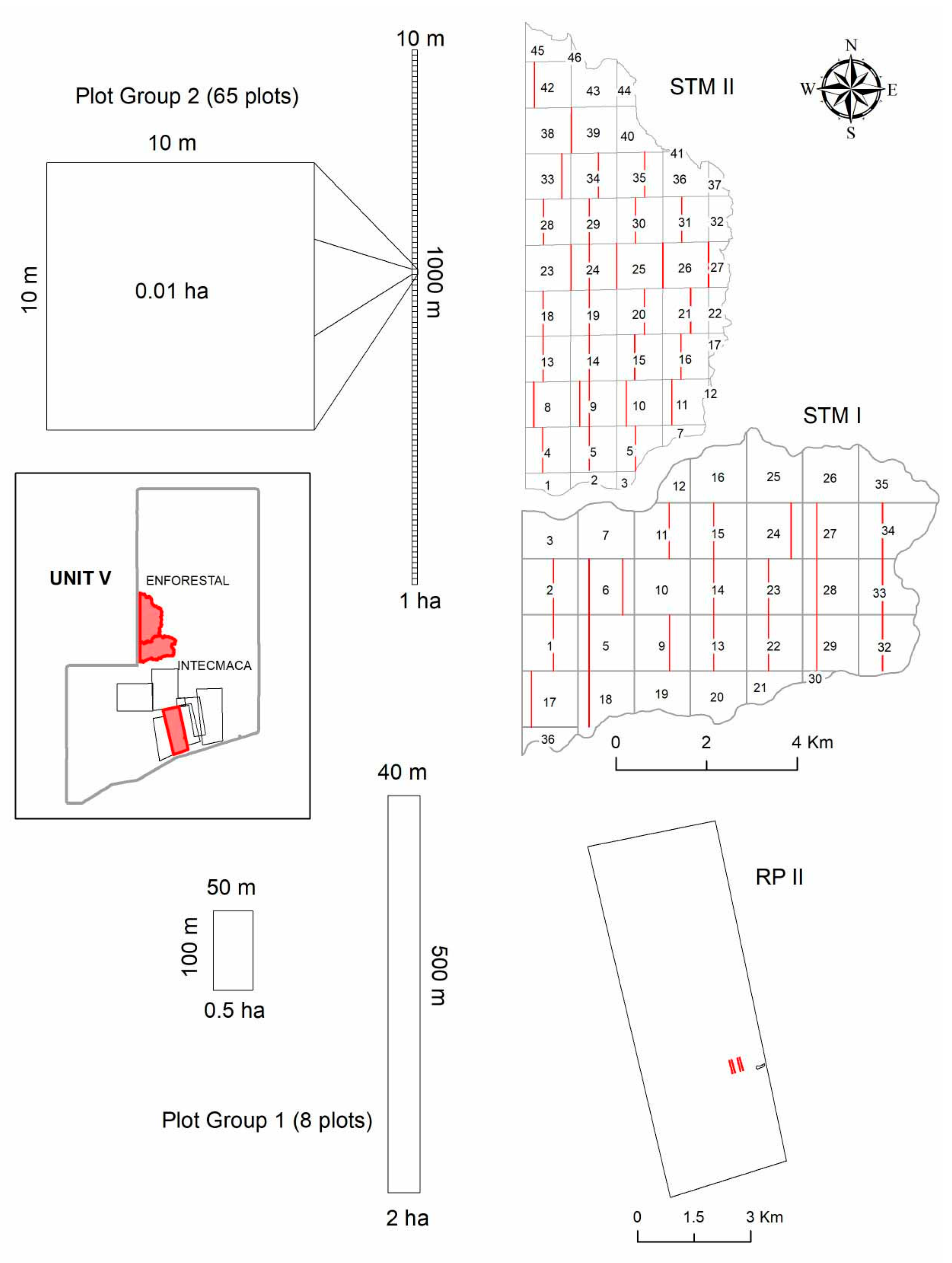
• The first group was obtained from INTECMACA inventories conducted between 1986 and 1995. Two groups of permanent plots were established in RP II: four plots of 0.5 ha (100 × 50 m) located in unlogged forests and four plots of 2 ha (500 × 40 m) in logged forests. The data include all living trees with diameters at breast height (dbh) > 10 cm [13,60].
• The second set of data was obtained from ENAFOR inventories conducted between 2012 and 2015. A group of temporary and permanent plots was systematically established in the STM I and STM II logging subunits; a total of 65 plots of 1 ha (1000 × 10 m) with subplots of 0.01 ha (10 m × 10 m) were measured in the pre- and post-logging periods [61,62] (Figure A1 in Appendix A). In all cases, a complete taxonomic identification was made to every individual to account for species composition and diversity.

In addition, official reports from the logging companies were used to collect data on the number and size of the harvested trees (diameter, height and species) [63]. Total volume per tree was estimated using the Smalian scale formula (cm³), so total volume of wood harvested at the compartment level could be estimated.

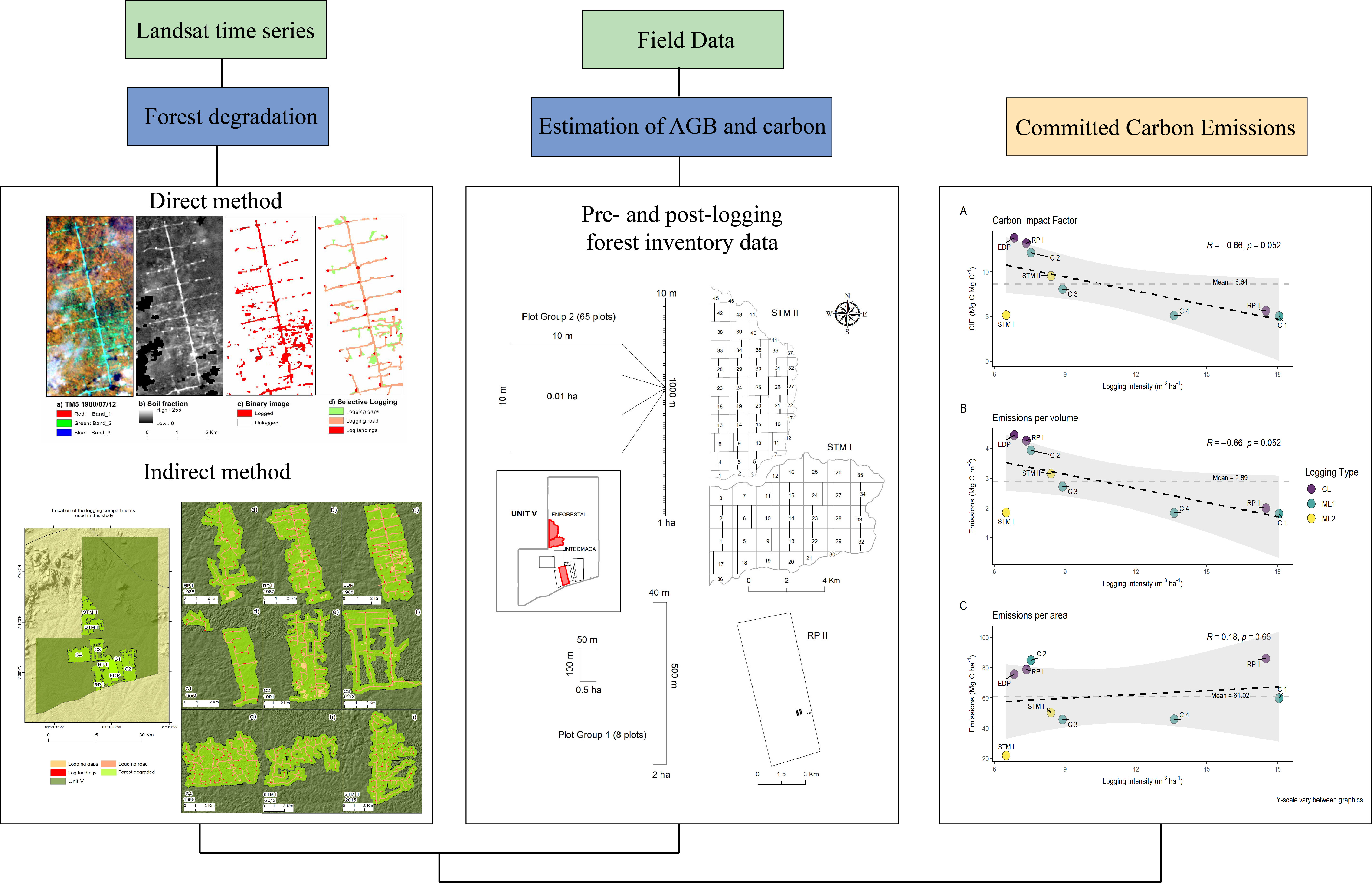
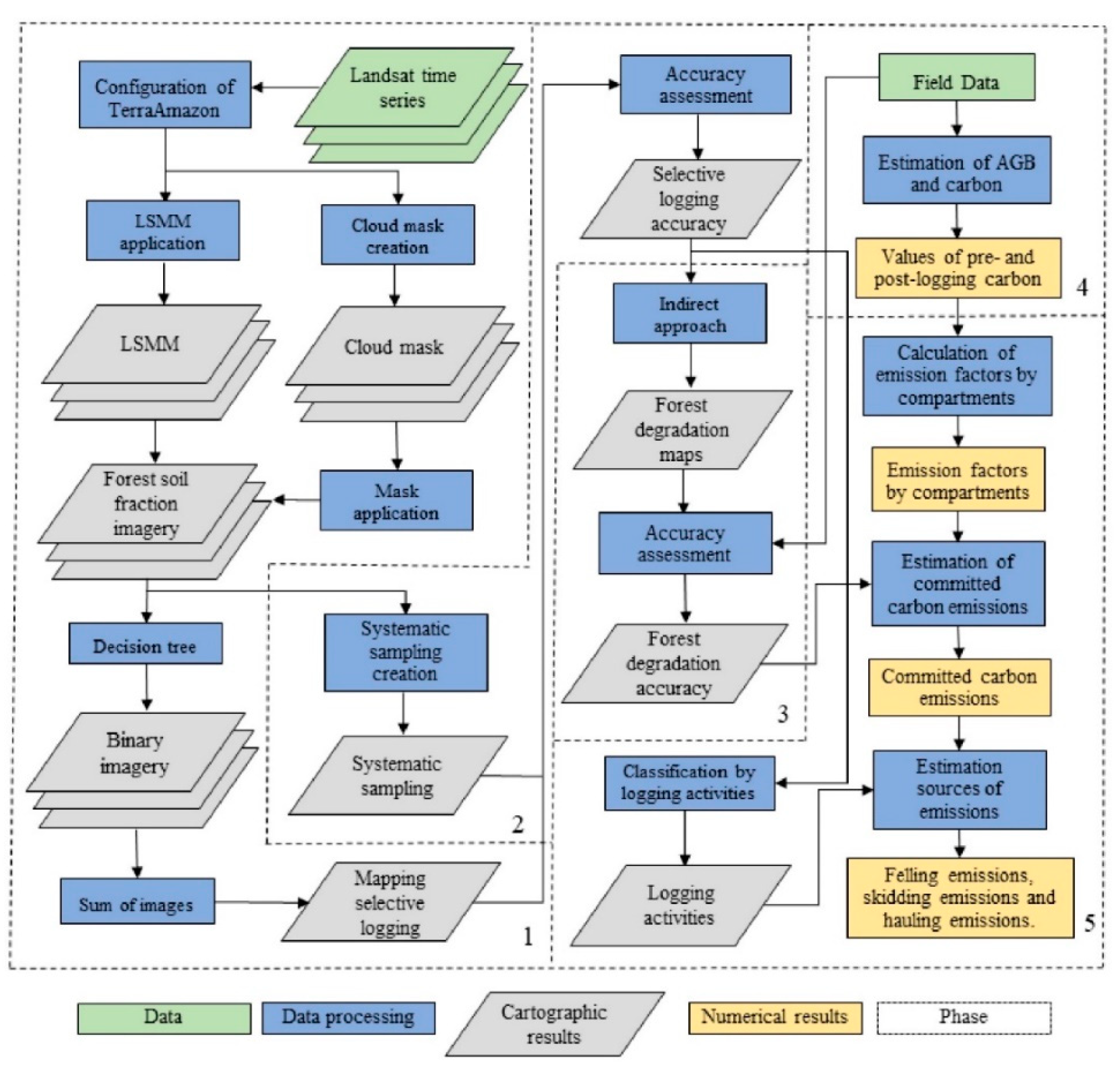
2.4. Analytical Approach

Our analytical approach consisted of five different phases as follows: we first mapped selective logging, followed by a validation process of the resulting maps. The third phase consisted of the construction and validation of the forest degradation maps, followed by the estimation of aboveground biomass (AGB) and carbon to close with the estimation of committed carbon emissions (CCE) (Figure 2).

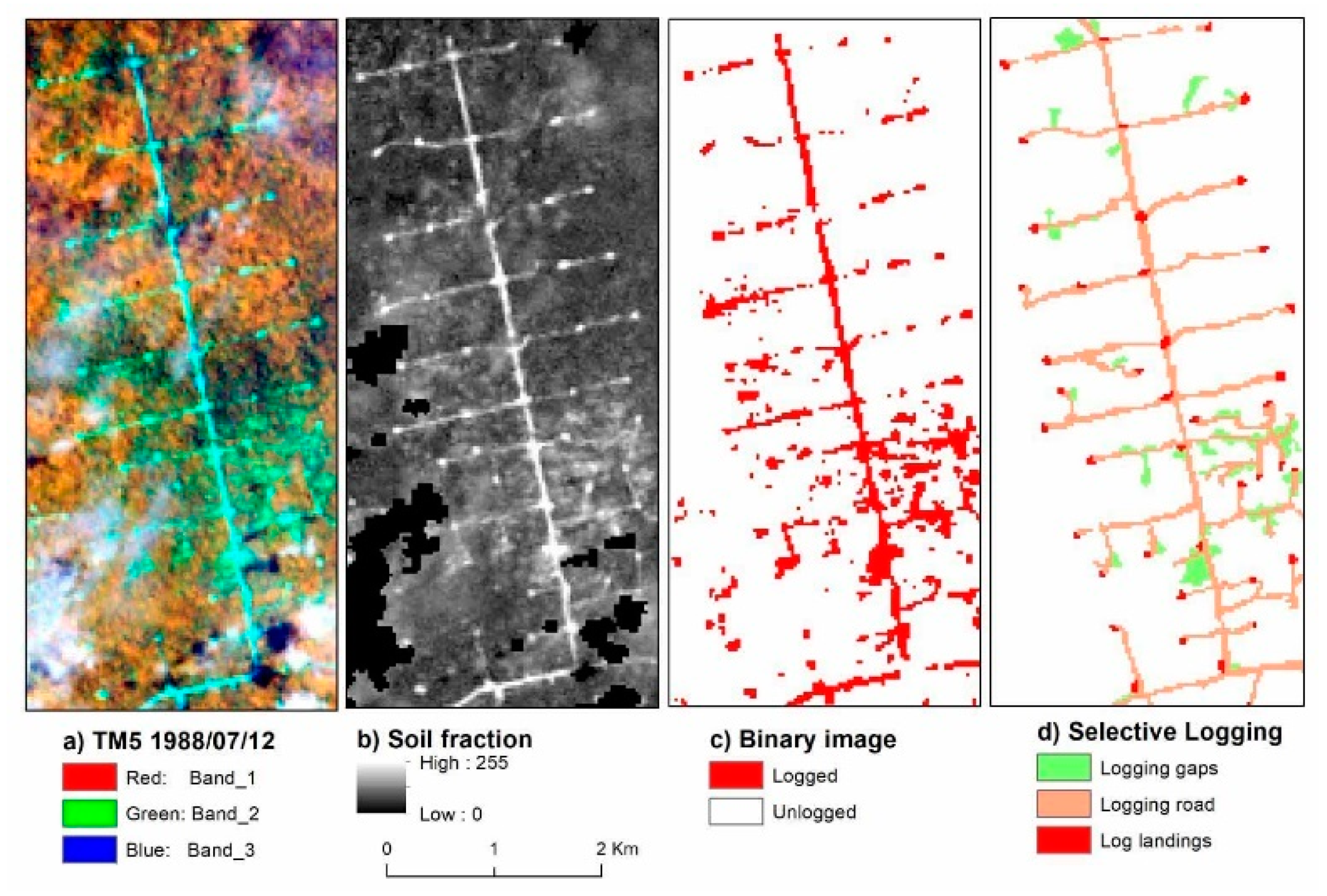
2.4.1. Mapping Selective Logging

The TerraAmazon system was used to map selective logging. This system involves a configuration that includes the creation of a PostgreSQL database, definition of the conceptual model, access control, phase control, project and control rules, definition of classes, definition of the control rules, and the definition of the control area [64]. The Landsat time series datasets were then exported to generate a linear spectral mixing model (LSMM) for each image to be used in the detection of selective logging [14,43,45,48,49]. The LSMM uses the red (0.63–0.69 μm), near infrared (0.76–0.90 μm) and mid-infrared (1.55–1.75 μm) bands from Landsat 4, 5, 7 and 8 [44], from which the samples of soil cover, vegetation and shade can be extracted to estimate the proportions in each pixel and in their respective images (Equation (1)). The soil fraction image was then used to estimate the area affected by selective logging [43,44,48,49,65].

$$r_i=a*ve{g}_i+b*soi{l}_i+c*shado{w}_i+e_i$$

(1)

where

• r_i = is the response of the pixel in band i;
• a, b, and c = proportions of vegetation, soil, and shade, respectively;
• vege_i, soil_i and shadow_i = spectral responses of the components of vegetation, soil and shade, for each band respectively;
• e_i = is the error in band i.

A cloud mask and cloud shadow were applied to each image of the soil fraction, using thresholds of the minimum and maximum values of the blue band (0.45–0.51 μm) to detect shadows and the infrared thermal band (10.60–11.19 μm) to detect clouds [64,66]. Selective logging was detected by means of a binary classification of areas with and without selective logging based on the processed images of the soil fraction [44,49]. A value of zero was assigned to those pixels with soil fractions lower than 37% (i.e., areas without evidence of selective logging), and a value of one corresponded to the pixels with soil fractions between 37 and 100% (i.e., areas with signs of selective logging). A decision tree algorithm was then used, for which the 37% limit was statistically defined based on 150 points visually selected from a processed soil fraction image [49]. Once the binary images were obtained, these were added to generate the mapping of selective logging.

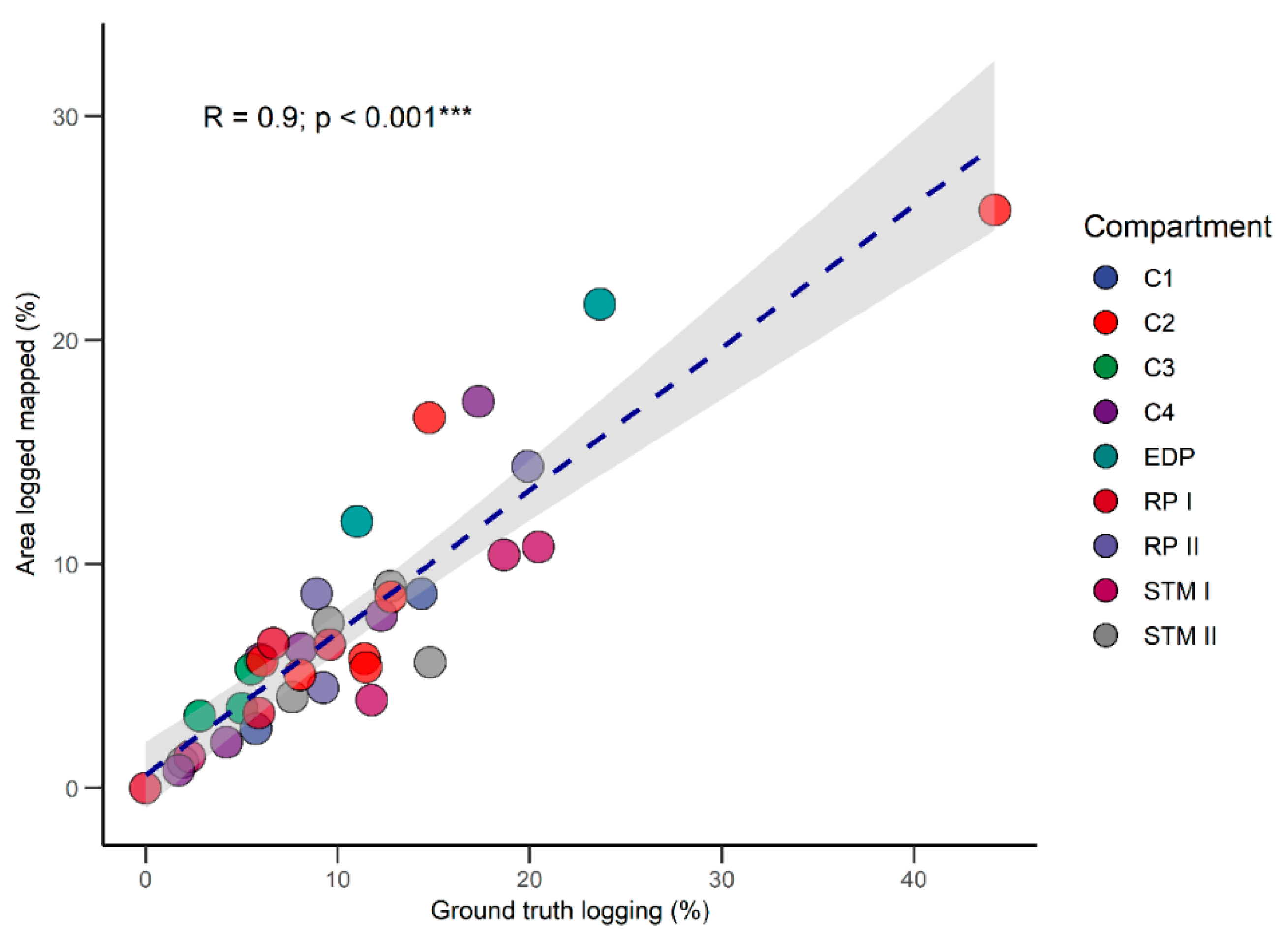
2.4.2. Validation of the Selective Logging Maps

To determine the quality and degree of agreement between the mapping of selective logging and field conditions, maps were validated via the comparison with an external source that is considered a realistic representation of the characteristics on the ground [67,68,69,70]. Thus, we applied a systematic sampling approach [50,71] to 36 blocks of 100 ha (1 km²) [72], which represented approximately 11% of the study area. This sampling technique allowed us to precisely and quickly estimate the error of the analysis [67,73]. By using a visual on-screen interpretation of a minimum cartographic area of 1 ha in each sampling block [72] we can generate logged and unlogged forest datasets (Figure A2 in Appendix A). These were considered the ground-truth data and were then used to analyze the thematic quality of the selective logging map. A confusion matrix was generated and the errors of omission and commission with the level of global accuracy were also calculated.

To confirm the logged classification, a spatially non-localized analysis was used by comparing the proportions of the area in each sample block in the selective logging map and in the ground-truth data. These proportions were compared via simple linear regression, with the rationale that if the mapping of selective logging and ground-truth data were similar, adjustment values would be high and the coefficient (R²), would be close to 1 [67,74]. This method has been widely used in the mapping of forest fires [75,76], analyses of land use [74] and deforestation [77].

2.4.3. Construction and Validation of the Forest Degradation Maps

Using an indirect method, mapping of forest degradation was performed for each logging compartment. In doing so, we estimated the average radius between log landings in each of the soil fraction images as proposed by Monteiro et al. [48]. In our case, this value was 600 meters (m), so 300 m was used as a threshold to estimate the approximate area of forest degradation caused by logging, and a square buffer was applied to the mapping of selective logging using GIS tools. Maps of forest degradation were validated by comparing these with the area logged reported in the management plans, which allowed for the calculation of commission and omission errors [68].

2.4.4. Estimation of Aboveground Biomass (AGB) and Carbon

Forest inventory data for pre- and post-logging conditions were used to estimate AGB and carbon, following the approach by the Global Observation of Forest and Land Cover Dynamics panel (GOFC-GOLD) [46] for the establishment of REDD+ projects. The AGB per tree in each ground plot was estimated using the pantropical allometric regression from Chave et al. [78] (Equation (2)). All the estimates were generated for each plot and the estimations were scaled to 1 ha when necessary. Values of aboveground carbon (Mg C ha⁻¹) were assumed to be 50% of AGB [79].

$$\begin{gathered} {\left(AGB\right)}_{est}=\exp \left(-1.803-0.976E+0.976ln\left(\mathsf{\rho }\right)+2.673\ln \left(\mathrm{D}\right) \\ -0.0299{\left(\ln \left(\mathrm{D}\right)\right)}^2\right) \end{gathered}$$

(2)

where:

AGB = is the aboveground biomass of the individual trees expressed in kilograms (kg); E = is a water stress factor that shows an important covariance with the diameter-height ratio in tropical trees and includes information on seasonal temperature (ST) and the climatic water deficit (CWD). Based on the geographic location of each plot, E and CWD were derived from a 2.5 arc-minute resolution raster file available at http://chave.ups-tlse.fr/pantropical_allometry.htm. (accessed on 10 March 2021); ρ = is the density of the wood in g cm⁻³, with data assigned for each taxonomic group from the pantropical database of Zanne et al. [80] and Chave et al. [81]; D = is the diameter of each tree in cm.

2.4.5. Estimation of Committed Carbon Emissions (CCE)

A stock-difference method was used to estimate emissions related to selective logging following the 2019 refinement of the 2006 IPCC guidelines [39]. In doing this, the following assumptions were considered:

• To simplify the carbon accounting process, the committed emissions approach was used, in which all carbon removed is assumed to be emitted at the time of its removal via logging [37,39].
• Emissions were estimated in each compartment by multiplying the area affected by degradation (activity data) with the difference of the carbon content in the pre- and post-logging period (emission factor) [39].
• The different harvesting activities were classified in the selective logging map into: log landings, caused when the forest is cleared for the purpose of temporary log storage before final transportation; logging roads, built to transport timber from log landings to sawmills; and logging gaps, created by tree felling and skid trails, resulting in damage or death to other standing trees [18,46]. These categories were associated with the emissions in each compartment to determine the overall emission contribution for each activity.
• Using the reported values of timber extracted from each compartment, carbon losses from logging were estimated by calculating the equivalent carbon of the volume of extracted roundwood, which considered the wood specific density to obtain AGB. A factor of 0.5 was used to estimate the amount of carbon [79,82].
• To adapt our data categories to the gain and loss method proposed by the IPCC [39] and used in Pearson et al. [37] and Ellis et al. [10], we linked the data to three main sources of emissions as follows: (1) roundwood extracted and felling emissions; (2) logging gaps and skidding emissions; (3) log landings and roads with hauling emissions.
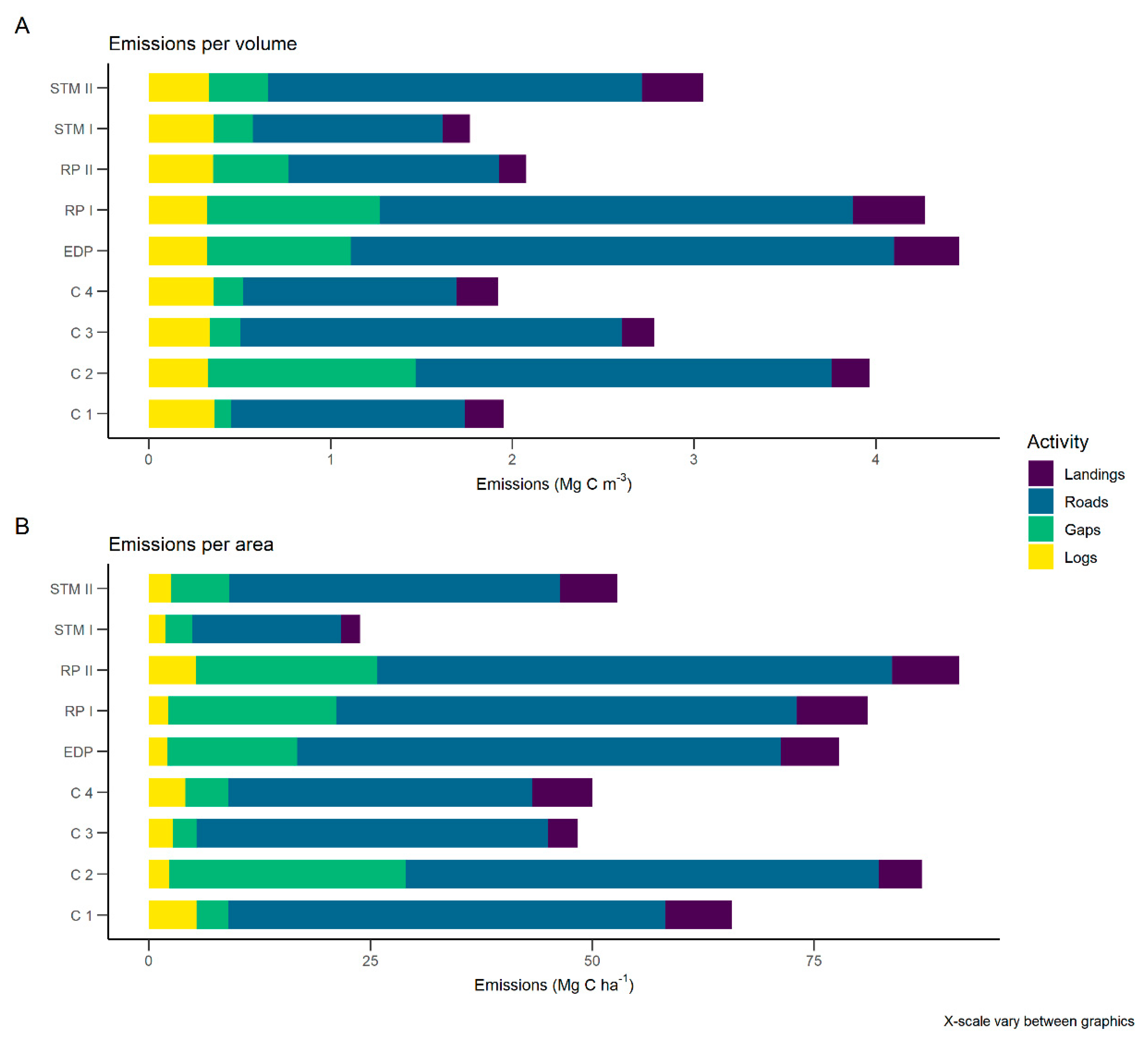
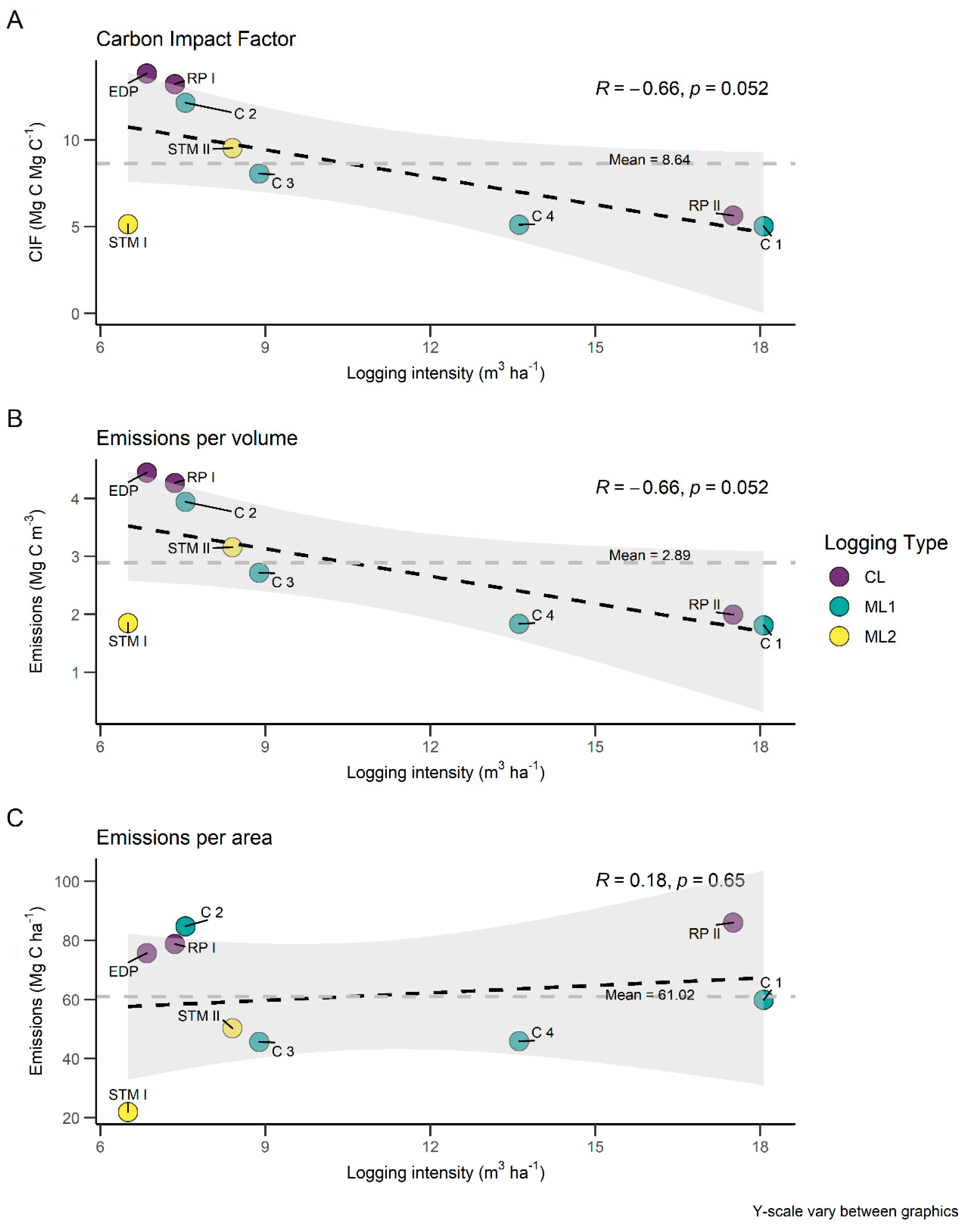
• We express carbon emissions in three ways: (1) emissions per area (Mg ha⁻¹) by dividing all emissions from each compartment using the estimated area of degradation [83]; (2) emissions per volume of harvested roundwood (Mg m⁻³), dividing all emissions from logging in each compartment by the total volume extracted [10]; (3) the carbon impact factor (CIF) (Mg Mg⁻¹) also called “mean carbon export ratio” [82], represents the emissions of each compartment relative to the emissions of the total volume of extracted roundwood.

3. Results

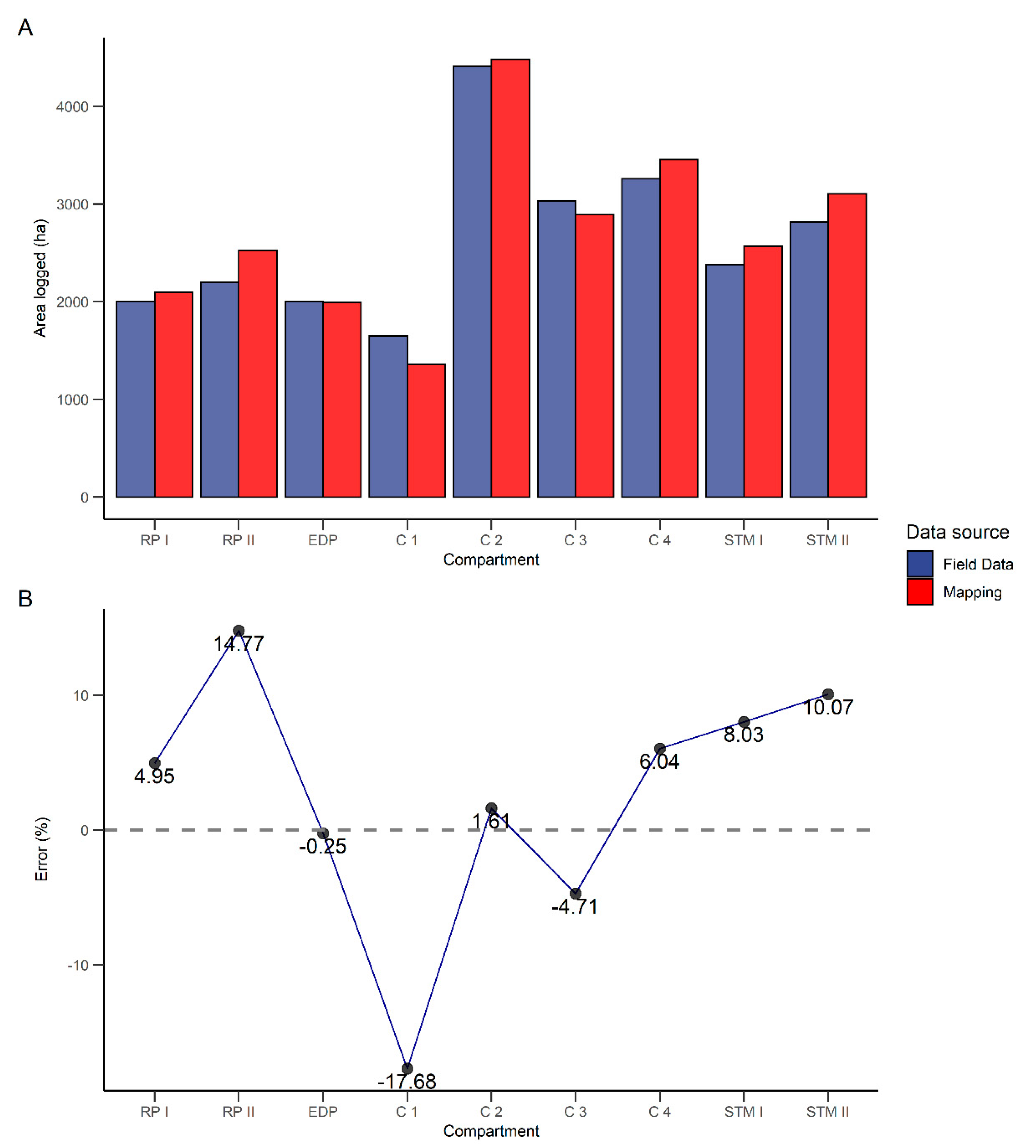
3.1. Accuracy of Maps of Selective Logging and Forest Degradation

The results from the error matrix are presented in terms of area proportions. The row totals of the error matrix (Sum = 0.113) provide what was represented in the ground-truth samples in each class and constitutes the total proportion of selective logging. Conversely, the column totals provide the estimated proportions according to the ground-truth data, and this was estimated in 0.013 for the logged class. Multiplying this value by the total number of pixels on the map (i.e., 330,386), the result is 4158 pixels, or approximately 374 ha. The area of agreement between the mapping of selective logging and the ground-truth data was 2452 pixels or close to 221 ha. There was an underestimation of 1706 pixels or around 154 ha that was confused with the unlogged class. On the other hand, the logged class had the highest user error (commission), with a proportion of 0.146, and a producer error (omission) of 0.4103 because greater proportions of areas were included and excluded in this class, respectively (

Table 2. The error matrix, omission and commission errors, and overall precision in terms of estimated area proportion.

Ground Truth (Proportion)
Class	Logged	Unlogged	Total
Logged	0.007	0.001	0.009
Unlogged	0.005	0.099	0.105
Total	0.013	0.101	0.113
Error
Commission	0.146	0.049
Omission	0.410	0.013
Global Precision	0.943

). The proportion of these errors was observed in nine of the 36 blocks that were used in the validation, three for the case of ENAFOR and six for INTECMACA (Figure A3 in Appendix A). The global precision of the selective logging map was 0.943.

The values of the ground-truth proportions and those of the mapping of selective logging showed an overall good fit. The proportions presented high similarity, as indicated by a high value in the coefficient of determination after a simple linear regression (R² = 0.82) (Figure A4 in Appendix A). In relation to the area of forest degradation obtained from the map, this represented approximately 13.6% (24,484 ha) of the entire area of Unit V. Analyzing this area for each compartment, six had commission errors, ranging from +1.6% in compartment C2 (71 ha) to +14.7% in compartment RP II (325 ha), while three compartments had errors of omission, ranging from −0.3% in compartment EDP (5 ha) to −17.7% in compartment C1 (292 ha) (Figure A5 in Appendix A).

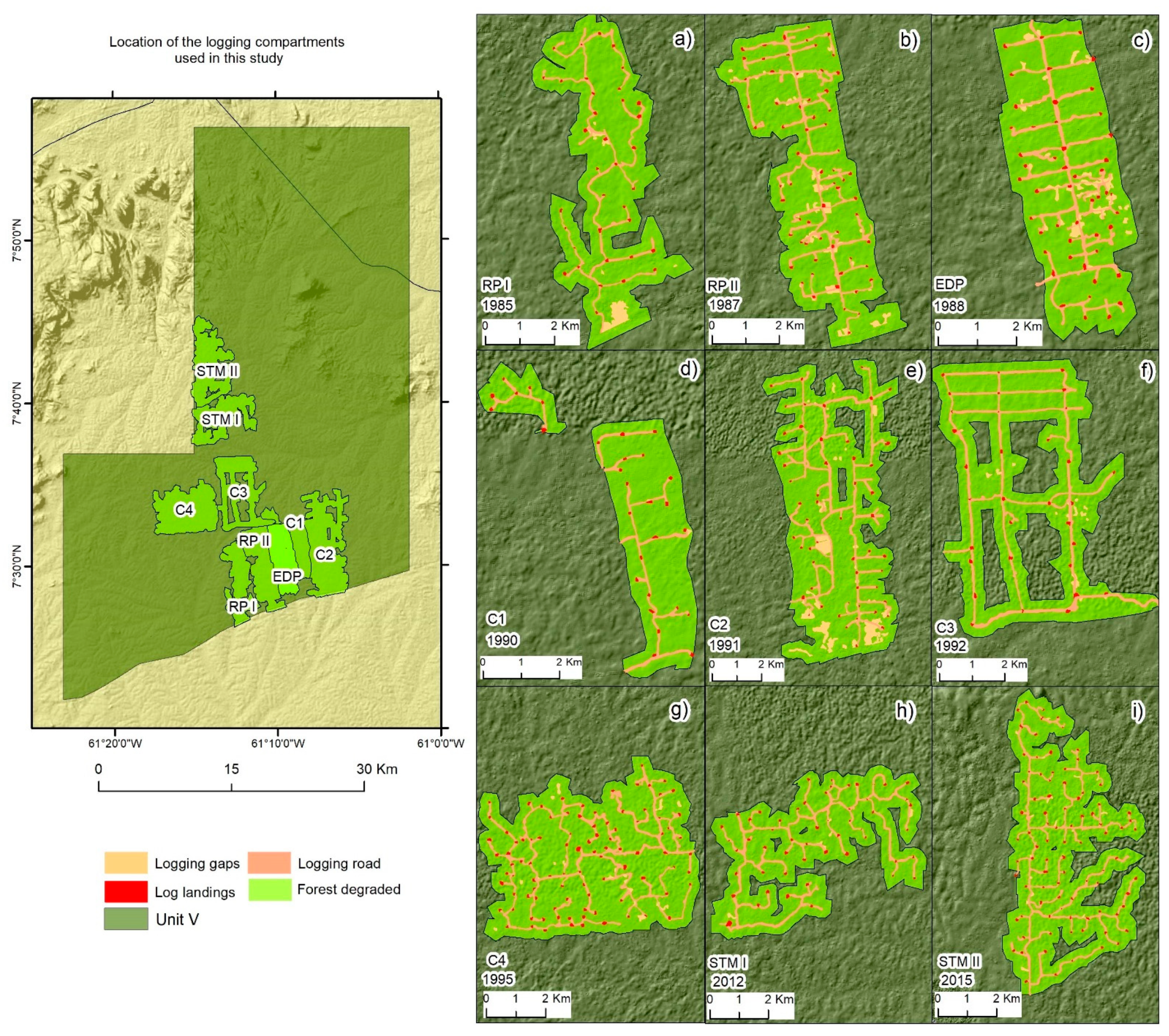
3.2. Mapping Selective Logging at Imataca Forest Reserve

Figure 3 shows the full process to detect and outline selective logging activities for the case of the EDP compartment (i.e., experimental development plot), logged during the first three months of 1988.

The total area directly affected by selective logging-related activities was around 2535 ha, from which compartment C2 had the largest area with 539 ha (21.2% of total area) and compartment C1 the lowest with 89 ha (3.5%), with an overall mean area of forest degradation of 282 ± 124 ha (±SD). The number of log landings built was, on average, 2.1 ± 0.6 (±SD) per 100 ha, with a total area of 2926 ± 496 m² and an area affected by logging of 59 ± 16 m² ha⁻¹. In terms of the extension of logging roads, we estimated an average of 16 ± 2.3 m ha⁻¹ in length, and a disturbed area of roads close to 583 ± 109 m² ha⁻¹. Finally, the average area affected in logging gaps was estimated at 174 ± 111 m² ha⁻¹ (

Table 3. General description of the area disturbed by construction of log landings, roads, and logging gaps in each compartment by logging approach in Unit V, Imataca Forest Reserve, Venezuela.

	Compartments a
	Unplanned Conventional Logging (CL)			Planned Logging 1 (ML1)				Planned Logging 2 (ML2)
	RP I	RP II	EDP	C 1	C 2	C 3	C 4	STM I	STM II
Loglandings
Number of log landings per 100 ha logged	1.7	2.6	2.5	2.1	1.2	1.1	2.7	2.1	2.9
Mean area of log landings (m2) ± SD	2690 ±1183	2317 ±935	2825 ±1073	2614 ±1018	3485 ±1774	3650 ±1563	3324 ±1345	3133 ±2139	2297 ±925
Log landings area per ha logged (m2 ha−1)	46.1	59.7	69.4	55.7	41.2	40.4	90.4	64.6	65.8
Logging roads
Length of logging road per hectare logged (m ha−1)	14	19	20	13	14	16	17	16	17
Logging road area per hectare logged (m2 ha−1)	404	617	769	448	605	642	625	601	533
Logginggaps
Area of gaps per total area logged (m2 ha−1)	184	278	254	41	378	64	106	153	105

^a Compartments: RP I: Research plot I; RP II: Research plot II; EDP: Experimental Development Plot; C1: Compartment 1; C2: compartment 2; C3: Compartment 3; C4: Compartment 4; STM I: Santa Maria I; and STM II: Santa Maria II.

). Spatial patterns of the different areas affected by logging were highly heterogeneous across all compartments. More regular arrangements, especially in terms of road building and distribution, seem clearer in the case of the oldest logging operations (e.g., RP1, RP2, EDP) in contrast with the most recent logged areas (i.e., STM I, STM II) (Figure 4).

3.3. Analysis of Forest Degradation

The total area of forest degradation caused by selective logging activities was estimated in 24,484 ha. The average area of forest degradation by compartment was 2720 ± 911 ha (Mean ± SD), with a maximum value of 3457 ha for compartment C4 and a minimum of 1360 ha in compartment C1 (Figure 4;

Table 4. General characteristics of the harvesting operations and the area affected in each compartment classified by activity and logging approach.

	Compartments a
	Unplanned Logging (CL)			Planned Logging 1 (ML1)				Planned Logging 2 (ML2)
	RP I	RP II	EDP	C 1	C 2	C 3	C 4	STM I	STM II
Year of logging	1985	1987	1988	1990	1991	1992	1995	2012	2015
Area of forest degradation (ha)	2099	2525	1995	1360	4480	2892	3457	2571	3105
Total number of trees logged	4000	11,458	5566	6116	10,240	5125	12,249	4345	5937
Total logged volume (m3)	15,433	44,207	13,650	24,566	33,804	25,695	47,073	16,639	25,967
Logging intensity 1 (trees ha−1)	1.9	4.5	2.8	4.5	2.3	1.8	3.5	1.7	1.9
Logging intensity 2 (m3 ha−1)	7.4	17.5	6.8	18.1	7.5	8.9	13.6	6.5	8.4
Log landings (%)	0.5	0.6	0.7	0.6	0.4	0.4	0.9	0.6	0.7
Logging roads (%)	4.0	6.2	7.7	4.5	6.1	6.4	6.3	6.0	5.3
Logging gaps (%)	1.8	2.8	2.5	0.4	3.8	0.6	1.1	1.5	1.0
Total area affected by logging (%)	6.3	9.6	10.9	5.4	10.2	7.5	8.2	8.2	7.0
Ground damage per tree logged (m2)	333	211	391	121	448	421	232	484	368
Ground damage per m3 of timber harvested (m2)	86	55	160	30	136	84	60	127	84

^a Compartments: RP I: Research plot I; RP II: Research plot II; EDP: Experimental Development Plot; C1: Compartment 1; C2: compartment 2; C3: Compartment 3; C4: Compartment 4; STM I: Santa Maria I; and STM II: Santa Maria II.

). In total, 65,036 trees were harvested in all compartments with a total volume of 247,034 m³, for a mean logging intensity of 2.8 ± 1.2 trees ha⁻¹ or 10.5 ± 4.6 m³ ha⁻¹. Average ground area damaged per tree logged was estimated in 334 ± 121.9 m², equivalent to 91 ± 41.9 m² for each cubic meter of timber harvested. The mean of the total area affected by logging represented 8.2 ± 1.8 % of the entire degraded area, 0.6 ± 0.2 % of this area corresponded to the construction of log landings, 5.8 ± 1.1 % to roads, and 1.7 ± 1.1 % to logging gaps (Table 4).

3.4. Aboveground Carbon Density

The values of forest carbon density for pre- and post-logging varied in the different compartments, with the pre-logging ranging from 268 Mg C ha⁻¹ (C4 compartment) to 312 Mg C ha⁻¹ (C2 compartment), with an average of 308 ± 76 (± SD) Mg C ha⁻¹. After logging, aboveground carbon density varied from 222 Mg C ha⁻¹ (RP I compartment) to 263 Mg C ha⁻¹ (STM I compartment), with an average of 229 ± 30 (± SD) Mg C ha⁻¹. The average difference between the two conditions was estimated in 35% (

Table 5. Density of carbon in the aboveground biomass by logging compartment in pre- and post-logging and average (including the mean ± standard deviation).

		Forest C Density (Mg C ha−1)
Compartments	Logging Method	Pre-Logging	Post-Logging	Difference (%)
RP I	CL	299 ± 76	222 ± 30	35
RP II	CL	300 ± 91	219 ± 23	37
EDP	CL	293 ± 76	220 ± 30	34
C 1	ML1	280 ± 29	225 ± 37	24
C 2	ML1	312 ± 76	229 ± 30	36
C 3	ML1	289 ± 7	246 ± 21	17
C 4	ML1	268 ± 29	226 ± 37	18
STM I	ML2	283 ± 7	263 ± 21	8
STM II	ML2	272 ± 29	224 ± 37	21
Average		308 ± 76	229 ± 30	35

).

3.5. Committed Carbon Emissions (CCEs) from Selective Logging

Mean CCEs per volume harvested was 2.9 ± 1.1 (mean ± SD) Mg C m⁻³, those from construction of logging roads were 1.9 ± 0.7 Mg C m⁻³ (64% of all emissions), logging gaps ~0.5 ± 0.4 Mg C m⁻³ (17% of all emissions), logged roundwood with ~0.3 ± 0.01 Mg C m⁻³ (10% of all emissions), and those from log landings ~0.2 ± 0.1 Mg C m⁻³ (9% all emissions). The maximum value was 4.4 ± 1.1 Mg C m⁻³ in the EDP compartment, and the minimum was 1.7 ± 0.4 Mg C m⁻³ from STM I compartment (Figure 5A). Mean CCEs per area for all selective logging activities was 64.2 ± 22.2 Mg C ha⁻¹. Logging road construction accounted for 43.9 ± 13.7 Mg C ha⁻¹ (68% of all emissions), logging gaps represented 11.3 ± 9.2 Mg C ha⁻¹ (18% of total), log landings accounted for 5.9 ± 2.0 Mg C ha⁻¹ (9%), and logged roundwood represented 3.2 ± 1.4 Mg C ha⁻¹ (5% of all emissions). The maximum value was estimated at 91.4 ± 24.4 Mg C ha⁻¹ in the compartment RP II, while the minimum was 23.8 ± 4.1 Mg C ha⁻¹ from the STM I compartment (Figure 5B).

CCEs for all nine compartments were highly variable. The CCEs expressed in terms of the Carbon Impact Factor (CIF), ranged between a minimum of 5.0 and a maximum of 13.2 Mg C Mg C⁻¹ for compartments C1 and EDP respectively, and their baseline was 8.6 ± 3.7 Mg C Mg C⁻¹. On a volume basis, CCEs ranged between 1.8 and 4.4 Mg m⁻³ for the case of C1, C4, STM I and EDP compartments, and their baseline was 2.9 ± 1.1 Mg m⁻³. On an area basis, CCEs ranged between 21.9 and 86.1 Mg ha⁻¹ for STM I and RP II compartments respectively, and their baseline was 61 ± 22 Mg ha⁻¹. The effect of the intensity of logging on CCEs was very similar in all three ways of reporting emissions (Figure 6). In terms of the logging approach, logging intensity values for the EDP and RP I compartments, where a conventional unplanned (CL) approach was common, were relatively low (between 6 and 8 m³ ha⁻¹), but the effects on carbon were above the baselines of the three ways of reporting emissions. In the case of the RP II compartment, logging intensity was high (17.5 m³ ha⁻¹) but below the CCEs baselines expressed either by volume or CIF. Planned selective logging 1 (ML1) used in compartments C1, C3 and C 4 had values below the baseline for all three ways of reporting emissions. However, the intensities increased from 8.3 m³ ha⁻¹ for compartment C3, 13.6 m³ ha⁻¹ for compartment C4 and 18.1 m³ ha⁻¹ for compartment C1, while in compartment C2 this intensity was low (7.5 m³ ha⁻¹) but its CCE values were still the highest. For planned selective logging 2 (ML2) applied in the compartment STM I, all values when reporting emissions were below the baseline, with an intensity of 5.2 m³ ha⁻¹, while compartment STM II the CCEs values by volume and CIF were above the baseline with an intensity of 8.4 m³ ha⁻¹ (Figure 6).

4. Discussion

4.1. Potential of the Analytical Approach

In this study we were able to develop a reliable and useful method to analyze selective logging via a local network using the Amazon Deforestation Monitoring System (TerraAmazon), with an architecture developed in a client-server environment, and with a TerraLib database which uses PostgreSQL as a Database Management System [52]. This analytical approach allowed us to estimate the area of forest degradation caused by selective logging with a high level of accuracy that subsequently help estimating the amount of carbon emissions produced.

Our results show the potential for this method to efficiently map selective logging automatically as shown in other studies [44,48,49,84,85]. With a relatively high global precision (GP = 0.943) that is within the range recommended by the GOFC-GOLD [46] for the development of forest cover monitoring maps, and slightly higher than that reported in the Brazilian Amazon (0.92) [49], and a high determination coefficient (0.82) that shows a close fit between the model and real proportions of the logging classes [67,74,77], we believe this is a promising and powerful tool to study forest degradation in tropical countries with severe connectivity limitations as the case of Venezuela.

Nonetheless, our study also confirms that detecting and mapping forest degradation with optical remote sensing data is a complex task, because the pixels that indicate forest degradation are an intricated mix of different land cover with diverse signals (i.e., vegetation, dead trees, bark, tree branches, soil, shadows, etc.) [45]. In addition, evidence of logging can rapidly disappear in less than two years after logging due to canopy closure and understory revegetation potentially limiting the overall accuracy of the method [18,41,58].

Mapping of forest degradation caused by selective logging yielded acceptable results, with average commission and omission errors of +7.6 ± 4.5 % (mean ± SD) and −7.5% ± 9.1 respectively, well below the uncertainty threshold of ±20% of the estimate for area [46], and of the results reported for the Brazilian Amazon (18% and 20%) [18] and the entire Amazon region (12% and 32%) [40].

The use of a relatively simple GIS model where the average of the log yarding radius was used, as in other studies [48,49], obeys to the fact that the Landsat time series for this area of the Amazon was not robust enough. Large proportions of clouds and cloud shadows covering the images [86], and the fairly low number of images available during the 1980s and 1990s [87] limited the use of spectral indices specialized in forest degradation such as the Normalized Degradation Fraction Index (NDFI) [18,41] and Continuous Degradation Detection (CODED) [40], or other more specialized statistical indices such as the Forest Degradation Index (FDI), based on a Multi Criteria Decision Analysis (MCDA) approach using the Analytic Hierarchy Process (AHP) technique [88,89]. Indeed, a similar result was found in a recently study on forest degradation in the Amazon using the NDFI [40], where forest degradation was marginally detected in our study area, sometimes overlapping with deforested areas.

The radius of the storage yards used by this indirect method (300 meters) to determine the buffer areas is slightly lower than in the case of other forest-types with lower densities of commercial tree species in the central and southern Amazon where 350 m was used as a threshold [48]. Our number of 300 m is, however, higher than the 180 m buffer zone used in a study carried out in dense tropical forests in the south-central Amazon [49]. Although stands of Unit V at IFR are often dense to moderately dense with an average volume of commercial trees of 33 m³ ha⁻¹ [57], compared to 20 m³ ha⁻¹ for transitional forests [48] and the 38 m³ ha⁻¹ for dense forests [49], we argue that an intermediate threshold value can reflect the fact that logging intensity was overall low in this unit of the Imataca Forest Reserve (IFR).

4.2. Selective Logging Detection

The use of Landsat images with a spatial resolution of 30-m has been a common approach in other studies analyzing the effects of selective logging [41,45,51,90,91,92], so these results are useful to compare the degree of agreement with our estimates. For instance, the mean mapped size of the log landings in our study area was 2926 ± 496 m² (mean ± SD), 17% higher than the originally planned area of 2500 m² (50 × 50 m) [56,61]. Despite this, the mean size mapped is within the range (1–4 pixels) of log landings detection in the soil fraction image [48], since approximately 3.3 pixels were detected.

In our study area, log landings were approximately nine times larger than those reported in southern Brazilian Amazonia (339 ± 31 m²) for reduced impact logging (RIL) operations. Regarding the number of log landings, we found that for every 100 ha, a mean of 2.1 ± 0.6 landings was created, equivalent to a disturbed area of 59 ± 16 m² ha⁻¹. These estimates largely differ from those reported for RIL in the Brazilian Amazon by Feldpausch et al. [82], where for every 100 ha, a higher density of log landings was created (6.2 ± 0.4), but with a much lower area disturbed of 20.8 ± 1.2 m² ha⁻¹. We interpret these results as a reflection of the overall poor planning and practical operationalization of logging activities in the case of IFR in comparison with RIL operations in other parts of the Amazon.

With regards to the effects of construction of logging roads, the management plans indicate a maximum width of 10 meters for main roads and 5 meters in the case of secondary roads plus an extra 10 m portion at each side for shoulder and ditch purposes in both type of roads [56,61,93,94]. Our mapping analysis shows that the mean length of all roads mapped was 16 ± 2.3 m ha⁻¹ and the disturbed area was 583 ± 109 m² ha⁻¹. If we consider that all the roads were established with an average of 30 m, the equivalent disturbed area that should have been expected would be around 483 ± 69 m² ha⁻¹, indicating a potential overestimation of ~21%. This overestimation can be interpreted as a result of the inaccuracies in the measurements of these areas due to the effect of the pixel size [18].

The average disturbance of logging gaps indicates a large variability in the total area disturbed (i.e., 174 ± 111 m²) likely a direct response of the different densities of commercial trees that can be found in this type of forests and the subsequent effects that felling and hauling one or more logged trees can have on the overall structure of the unlogged portion of the forest stands [36,94].

4.3. Relationship between Logging Intensity and Degradation

We found no significant differences between the CL and ML1 harvesting modalities (3.1 ± 1.3 trees ha⁻¹ and 3.0 ± 1.2 trees ha⁻¹ respectively). However, the ML2 modality was significantly different (1.8 ± 1.2 trees ha⁻¹), likely a consequence of the increase made to the minimum harvest diameters (MHD) for this compartment [57]. Overall, logging intensity was relatively low and similar to other management units in the IFR [53,54]. Compared to other areas in the Amazon, logging intensity at IFR is lower (e.g., 4.4 trees ha⁻¹—Jackson [95]; 4.5 trees ha⁻¹—Johns et al. [96]; 6.4 trees ha⁻¹—Verissimo et al. [97]), which can be explained by the differences in species composition and the abundance of commercial species among these areas.

Considering the different approaches of selective logging applied in our study case, the proportion of aboveground biomass (AGB) affected by logging was 35 ± 1.7% for the CL modality, below the 60% reported for other conventional logging cases in Amazonian forests [18,59]. In the case of planned logging, the average AGB damaged was 24 ± 8.5% for ML1 and 14.5 ± 9.7% for the ML2 case, above and below respectively compared with an overall 20% reported for this type of logging [18,59]. In general, all three modalities of logging were within the ranges of effects to living biomass (10–46%) found in other studies [97,98,99].

Of the total area of forest degradation (24,484 ha), the mean area affected by selective logging that was detected by the direct method was 8.2 ± 1.8%, slightly lower than the 10.2 ± 1.2% [100] and 13 ± 4.5 (SD) % [82], reported for the eastern and southern Brazilian Amazonia respectively, where reduced impact techniques were applied.

Logging disturbances were not homogeneous in each compartment and within the different types of logging. In some cases, however, by increasing the minimum harvest diameter (MHD), the logging intensity declined but not the proportion of area disturbed, such as the case of ML2 where MHDs were stratified by specific wood density. A potential explanation for these discrepancies can be found in the fact that while a lower number of trees were harvested, their average size also increased. Thus, without an adequate planning for liana removal prior to logging or the sufficient application of directional feeling during harvesting there is potential for a much larger disturbance effect [101].

4.4. Pre and Post Logging Aboveground Biomass (AGB) and Committed Emissions (CCE)

If the AGB is averaged prior to logging, the value obtained is 308 ± 76.3 Mg ha⁻¹, which coincides with several studies in humid tropical lowland forests of the Venezuelan Amazon [12,13,31,32,102]. Logging across all compartments reduced pre-disturbance AGB, on average, by 35% with higher values found for the unplanned logging approaches as expected (Table 3; Figure 6). While the characteristics of the logging at each compartment are unique, it is encouraging to see a lower reduction in carbon losses when selective logging includes a better preparation. However, it must be noted that a lower damage is not always a response of better planning. Instead, it can also be a direct response to the spatial aggregation of commercially valuable timber trees along with topographical conditions and other biophysical/economic factors that are particular at each site and at the time when logging occurred (e.g., 1985 vs. 2015). For instance, in a recent review conducted across the tropics, Putz et al. [101] found that an average of 57% (range 22–97%) of the area in logging blocks was not directly affected by timber harvests, with more forests being left intact in areas farther from roads, on slopes >40%, and within 25 m of perennial streams. In addition, our study, as many others focusing on the impacts of selective logging in the tropics (e.g., Verissimo et al. [97]; Gerwing, [98]; Veríssimo et al. [99]) is mostly based on aggregated means of logging intensity, and that often can be a relatively weak reflection of the conditions on the ground [101].

In our analysis, CCEs both by sources (Figure 5) and those expressed by area, volume and impact factor (Figure 6) were higher compared to other parts of the tropics (e.g., [98,99,100]). This corroborates what has been discussed regarding the intensity and the logging methods used across these areas of the IFR, highlighting the widespread low efficiency compared to other cases where reduced impact logging is formally applied. Although beyond the scope of our work, the absence of formal criteria and indicators for monitoring forest management practices in Venezuelan managed forests that has been demonstrated previously [29], our results add new evidence about the inadequate planning of logging activities, which may further limit the potential of forest management to serve as a climate change mitigation tool.

5. Conclusions

Compared to other regions of the Amazon basin and the tropics in general, our research reveals that in the northeastern Venezuelan Amazon, while the overall harvesting intensity has remained low over long periods of time, the disturbances associated to logging were considerably high. Selective logging activities showed rather poor planning and low efficiency, reflected in the fact that, regardless of the metric used (area-based, volume-based or CIF), carbon emissions were higher than most studies focusing on similar questions.

Digital image processing and GIS techniques used within the TerraAmazon system, and in conjunction with the 2019 Refinement IPCC Guidelines, enabled us to develop, for the first time in Venezuela, a low-cost and robust analytical approach to study the relationships between selective logging, forest degradation and carbon emissions. Our work also reveals that the use of spectral contrast along with Landsat time series, and ground-based data are excellent tools for the analysis of forest degradation, the evaluation of the impact at the canopy level due to the different activities and modalities of selective logging, and for the estimation of carbon emissions. This study is a step forward to improve and plan other more detailed analytical techniques (e.g., Lidar-Light Detection and Ranging) and for establishing a baseline of carbon emissions in the context of sustainable forest management.

References

1. Blaser, J.; Sarre, A.; Poore, D.; Johnson, S. Status of Tropical Forest Management 2011; ITTO Technical Series; International Tropical Timber Organization: Yokohama, Japan, 2011. [Google Scholar]
2. Petrokofsky, G.; Sist, P.; Blanc, L.; Doucet, J.-L.; Finegan, B.; Gourlet-Fleury, S.; Healey, J.R.; Livoreil, B.; Nasi, R.; Peña-Claros, M.; et al. Comparative effectiveness of silvicultural interventions for increasing timber production and sustaining conservation values in natural tropical production forests. A systematic review protocol. Environ. Evid. 2015, 4, 8. [Google Scholar] [CrossRef] [Green Version]
3. Sist, P.; Rutishauser, E.; Peña-Claros, M.; Shenkin, A.; Hérault, B.; Blanc, L.; Baraloto, C.; Baya, F.; Benedet, F.; da Silva, K.E.; et al. The Tropical managed Forests Observatory: A research network addressing the future of tropical logged forests. Appl. Veg. Sci. 2015, 18, 171–174. [Google Scholar] [CrossRef] [Green Version]
4. Piponiot, C.; Rödig, E.; Putz, F.E.; Rutishauser, E.; Sist, P.; Ascarrunz, N.; Blanc, L.; Derroire, G.; Descroix, L.; Guedes, M.C.; et al. Can timber provision from Amazonian production forests be sustainable? Environ. Res. Lett. 2019, 14, 64014. [Google Scholar] [CrossRef]
5. Piponiot, C.; Rutishauser, E.; Derroire, G.; Putz, F.E.; Sist, P.; West, T.A.P.; Descroix, L.; Guedes, M.C.; Coronado, E.N.H.; Kanashiro, M.; et al. Optimal strategies for ecosystem services provision in Amazonian production forests. Environ. Res. Lett. 2019, 14, 124090. [Google Scholar] [CrossRef]
6. Putz, F.E.; Romero, C. Futures of Tropical Production Forests; Center for International Forestry Research (CIFOR): Bogor, Indonesia, 2015. [Google Scholar] [CrossRef]
7. Putz, F.E.; Zuidema, P.A.; Synnott, T.; Peña-Claros, M.; Pinard, M.A.; Sheil, D.; Vanclay, J.K.; Sist, P.; Gourlet-Fleury, S.; Griscom, B.; et al. Sustaining conservation values in selectively logged tropical forests: The attained and the attainable. Conserv. Lett. 2012, 5, 296–303. [Google Scholar] [CrossRef] [Green Version]
8. Putz, F.E.; Zuidema, P.A.; Pinard, M.A.; Boot, R.G.A.; Sayer, J.A.; Sheil, D.; Sist, P.; Elias; Vanclay, J.K. Improved Tropical Forest Management for Carbon Retention. PLoS Biol. 2008, 6, e166. [Google Scholar] [CrossRef] [PubMed] [Green Version]
9. FAO. Forest degradation and improvement. In Proceedings of the Second Expert Meeting on Harmonising Forest-Related Definitions for use by Various Stakeholders, Rome, Italy, 11–13 September 2002. [Google Scholar]
10. Ellis, P.W.; Gopalakrishna, T.; Goodman, R.C.; Putz, F.E.; Roopsind, A.; Umunay, P.M.; Zalman, J.; Ellis, E.A.; Mo, K.; Gregoire, T.G.; et al. Reduced-impact logging for climate change mitigation (RIL-C) can halve selective logging emissions from tropical forests. For. Ecol. Manag. 2019, 438, 255–266. [Google Scholar] [CrossRef]
11. Pearson, T.R.H.; Brown, S.; Murray, L.; Sidman, G. Greenhouse gas emissions from tropical forest degradation: An underestimated source. Carbon Balance Mana. 2017, 12, 3. [Google Scholar] [CrossRef] [Green Version]
12. Houghton, R.A. Aboveground forest biomass and the global carbon balance. Glob. Chang. Biol. 2005, 11, 945–958. [Google Scholar] [CrossRef]
13. Vilanova, E.; Ramírez-Angulo, H.; Torres-Lezama, A. El almacenamiento de carbono en la biomasa aérea como un indicador del impacto de la extracción selectiva de maderas en la Reserva Forestal Imataca, Venezuela. Interciencia 2010, 35, 659–665. [Google Scholar]
14. Asner, G.P.; Knapp, D.E.; Broadbent, E.N.; Oliveira, P.J.C.; Keller, M.; Silva, J.N. Selective Logging in the Brazilian Amazon. Science 2005, 310, 480–482. [Google Scholar] [CrossRef] [PubMed]
15. Hosonuma, N.; Herold, M.; De Sy, V.; De Fries, R.; Brockhaus, M.; Verchot, L.; Angelsen, A.; Romijn, E. An assessment of deforestation and forest degradation drivers in developing countries. Environ. Res. Lett. 2012, 7, 44009. [Google Scholar] [CrossRef]
16. Mollicone, D.; Achard, F.; Federici, S.; Eva, H.D.; Grassi, G.; Belward, A.; Raes, F.; Seufert, G.; Stibig, H.-J.; Matteucci, G. An incentive mechanism for reducing emissions from conversion of intact and non-intact forests. Clim. Chang. 2007, 83, 477–493. [Google Scholar] [CrossRef]
17. Pacheco, C.; Aguado, I.; Mollicone, D. Las causas de la deforestación en Venezuela: Un estudio retrospectivo. Biollania 2011, 10, 281–292. [Google Scholar]
18. Souza, C. Monitoring of Forest Degradation: A Review of Methods in the Amazon Basin. In Global Forest Monitoring from Earth Observation; Archard, F., Hansen, M.C., Eds.; CRC Press Taylor & Francis Group: Boca Raton, FL, USA, 2013; pp. 171–194. [Google Scholar]
19. Achard, F.; Stibig, H.J.; Eva, H.D.; Lindquist, E.J.; Bouvet, A.; Arino, O.; Mayaux, P. Estimating tropical deforestation from Earth observation data. Carbon Manag. 2010, 1, 271–287. [Google Scholar] [CrossRef] [Green Version]
20. Herold, M.; Roman-Cuesta, R.; Mollicone, D.; Hirata, Y.; Van Laake, P.; Asner, G.; Souza, C.; Skutsch, M.; Avitabile, V.; MacDicken, K. Options for monitoring and estimating historical carbon emissions from forest degradation in the context of REDD+. Carbon Balance Manag. 2011, 6, 13. [Google Scholar] [CrossRef] [Green Version]
21. UNFCCC. Decision 2/CP.13. Reducción de las Emisiones Derivadas de la Deforestación en los Países en Desarrollo: Métodos Para Estimular la Adopción de Medidas, Bali. 2007. Available online: http://unfccc.int/resource/docs/2007/cop13/spa/06a01s.pdf#page=8 (accessed on 19 January 2021).
22. Nationally determined contributions (NDCs). United Nations Framework Convention on Climate Change. In Proceedings of the COP 21 Climate Agreement. United Nations Framework Convention on Climate Change, Paris, France, 30 November–11 December 2015. [Google Scholar]
23. Kammesheidt, L.; Lezama, A.T.; Franco, W.; Plonczak, M. History of logging and silvicultural treatments in the western Venezuelan plain forests and the prospect for sustainable forest management. For. Ecol. Manag. 2001, 148, 1–20. [Google Scholar] [CrossRef]
24. Torres-Lezama, A.; Ramírez-Angulo, H.; Vilanova, E.; Barros, R. Forest resources in Venezuela: Current status and prospects for sustainable management. Bois Forêts Des Trop. 2008, 295, 21–33. [Google Scholar]
25. Centeno, J. Estrategia Para el Desarrollo Forestal en Venezuela; Fondo Nacional de Investigación Forestal: Caracas, Venezuela, 1995. [Google Scholar]
26. MINEC. Anuario Estadísticas Forestales 2017; MINEC: Caracas, Venezuela, 2018. [Google Scholar]
27. Food and Agriculture Organization of the United Nations (FAO). Global Forest Resources Assessment 2020 Key Findings 2020; FAO: Rome, Italy, 2020. [Google Scholar]
28. Torres, A. La cuidada movilización de los recursos forestales. La industria forestal. Medio humano, establecimientos y actividades. In Geo Venezuela; Tomo 3; Fundación Polar: Caracas, Venezuela, 2008; pp. 382–438. [Google Scholar]
29. Vilanova, E.; Ramírez-Angulo, H.; Ramírez, G.; Torres-Lezama, A. Compliance with sustainable forest management guidelines in three timber concessions in the Venezuelan Guayana: Analysis and implications. For. Policy Econ. 2012, 17, 3–12. [Google Scholar] [CrossRef]
30. Berroterán, J.L. Reserva Forestal Imataca, Ecología y Bases Técnicas Para el Ordenamiento Territorial; Ministerio del Ambiente y de los Recursos Naturales: Caracas, Venezuela, 2003.
31. Avitabile, V.; Herold, M.; Heuvelink, G.B.M.; Lewis, S.L.; Phillips, O.L.; Asner, G.P.; Armston, J.; Ashton, P.S.; Banin, L.; Bayol, N.; et al. An integrated pan-tropical biomass map using multiple reference datasets. Glob. Chang. Biol. 2016, 22, 1406–1420. [Google Scholar] [CrossRef] [PubMed] [Green Version]
32. Delaney, M.; Brown, S.; Lugo, A.; Torres-Lezama, A.; Bello-Quintero, N. The distribution of organic carbon in major components of forests located in five life zones of Venezuela. J. Trop. Ecol. 1997, 13, 697–708. [Google Scholar] [CrossRef]
33. Pacheco, C.; Aguado, I.; Mollicone, D. Identification and characterization of deforestation hot spots in Venezuela using MODIS satellite images. Acta Amaz. 2014, 44, 185–196. [Google Scholar] [CrossRef] [Green Version]
34. Pacheco, P.; Mo, K.; Dudley, N.; Shapiro, A.; Aguilar-Amuchastegui, N.; Ling, P.Y.; Anderson, C.; Marx, A. Deforestation Fronts: Drivers and Responses in a Changing World; WWF: Gland, Switzerland, 2021. [Google Scholar]
35. Pacheco-Angulo, C. Estimación de las emisiones evitadas directas e indirectas en los depósitos de biomasa terrestres de la RFI. In Protocolo para la Valoración Ambiental y Económica de la Reserva Forestal Imataca; Peréz, R., Ed.; Componente 1: Sistema Nacional Integrado de Información Forestal (SINIFF); Proyecto Ordenación Forestal Sustentable y Conservación de Bosques en la Perspectiva Ecosocial (GCP/VEN/011/GFF); MINEC: Caracas, Venezuela, 2019. [Google Scholar]
36. Ochoa, J. Análisis preliminar de los efectos del aprovechamiento de maderas sobre la composición y estructura de bosques en la Guayana venezolana. Interciencia 1998, 23, 197–207. [Google Scholar]
37. Pearson, T.R.H.; Brown, S.; Casarim, F. Carbon emissions from tropical forest degradation caused by logging. Environ. Res. Lett. 2014, 9, 1–11. [Google Scholar] [CrossRef] [Green Version]
38. Global Forest Observations Initiative (GFOI). Integration of Remote-Sensing and Ground-Based Observations for Estimation of Emissions and Removals of Greenhouse Gases in Forests; Methods and Guidance from the Global Forest Observations Initiative; Global Forest Observations Initiative; Group on Earth; Food and Agriculture Organization of the United Nations: Rome, Italy, 2020. [Google Scholar]
39. IPCC. 2019 Refinement to the 2006 IPCC Guidelines for National Greenhouse Gas Inventories; Calvo Buen.; IPCC: Bern, Switzerland, 2019. [Google Scholar]
40. Bullock, E.L.; Woodcock, C.E.; Souza, C., Jr.; Olofsson, P. Satellite-based estimates reveal widespread forest degradation in the Amazon. Glob. Chang. Biol. 2020, 26, 2956–2969. [Google Scholar] [CrossRef]
41. Bullock, E.L.; Woodcock, C.E.; Olofsson, P. Monitoring tropical forest degradation using spectral unmixing and Landsat time series analysis. Remote Sens. Environ. 2020, 238, 110968. [Google Scholar] [CrossRef]
42. Ota, T.; Ahmed, O.S.; Minn, S.T.; Khai, T.C.; Mizoue, N.; Yoshida, S. Estimating selective logging impacts on aboveground biomass in tropical forests using digital aerial photography obtained before and after a logging event from an unmanned aerial vehicle. For. Ecol. Manag. 2019, 433, 162–169. [Google Scholar] [CrossRef]
43. Pacheco-Angulo, C.; Vilanova, E.; Aguado, I.; Monjardin, S.; Martinez, S. Carbon emissions from deforestation and degradation in a forest reserve in Venezuela between 1990 and 2015. Forests 2017, 8, 291. [Google Scholar] [CrossRef] [Green Version]
44. Shimabukuro, Y.E.; Arai, E.; Duarte, V.; Jorge, A.; dos Santos, E.G.; Gasparini, K.A.C.; Dutra, A.C. Monitoring deforestation and forest degradation using multi-temporal fraction images derived from Landsat sensor data in the Brazilian Amazon. Int. J. Remote Sens. 2019, 40, 5475–5496. [Google Scholar] [CrossRef]
45. Souza, C.M.; Roberts, D. Mapping forest degradation in the Amazon region with Ikonos images. Int. J. Remote Sens. 2005, 26, 425–429. [Google Scholar] [CrossRef]
46. GOFC-GOLD. A Sourcebook of Methods and Procedures for Monitoring and Reporting Anthropogenic Greenhouse Gas Emissions and Removals Associated with Deforestation, Gains and Losses of Carbon Stocks in Forests Remaining Forests, and Forestation; GOFC-GOLD Report Versio; GOFC-GOLD Land Cover Project Office, Wageningen University: Wageningen, The Netherlands, 2016. [Google Scholar]
47. Souza, C.; Firestone, L.; Silva, L.M.; Roberts, D. Mapping forest degradation in the Eastern Amazon from SPOT 4 through spectral mixture models. Remote Sens. Environ. 2003, 87, 494–506. [Google Scholar] [CrossRef]
48. Monteiro, A.L.; Souza, C.M.; Barreto, P. Detection of logging in Amazonian transition forests using spectral mixture models. Int. J. Remote Sens. 2003, 24, 151–159. [Google Scholar] [CrossRef]
49. Souza, J.R.; Barreto, P. An alternative approach for detecting and monitoring selectively logged forests in the Amazon. Int. J. Remote Sens. 2000, 21, 173–179. [Google Scholar] [CrossRef]
50. Banskota, A.; Kayastha, N.; Falkowski, M.J.; Wulder, M.A.; Froese, R.E.; White, J.C. Forest Monitoring Using Landsat Time Series Data: A Review. Can. J. Remote Sens. 2014, 40, 362–384. [Google Scholar] [CrossRef]
51. Jackson, C.M.; Adam, E. Remote sensing of selective logging in tropical forests: Current state and future directions. iForest Biogeosci. For. 2020, 13, 286–300. [Google Scholar] [CrossRef]
52. TerraAmazon. Monitoring System of Deforestation in the Amazon; Fundação de Ciência, aplicações e Tecnologia Espacial and Instituto Nacional de Pesquisas Espaciais: São Paulo, Brazil, 2005. [Google Scholar]
53. CODEFORSA. Informe Plan Anual de Corta No 8. Unidad N-2 Reserva Forestal Imataca; El Palmar: Edo Bolívar, Venezuela, 2003. [Google Scholar]
54. COMAFOR. Plan de Ordenación y Manejo Forestal, Unidad C-3 Reserva Forestal Imataca; Consorcio Maderero Forestal C.A. Upata, Estado Bolívar.Varios tomos; COMAFOR: Upata, Venezuela, 1994. [Google Scholar]
55. Piponiot, C.; Sist, P.; Mazzei, L.; Peña-Claros, M.; Putz, F.E.; Rutishauser, E.; Shenkin, A.; Ascarrunz, N.; de Azevedo, C.P.; Baraloto, C.; et al. Carbon recovery dynamics following disturbance by selective logging in Amazonian forests. Elife 2016, 5, e21394. [Google Scholar] [CrossRef] [PubMed]
56. INTECMACA. Plan de Ordenación y Manejo Forestal de la Unidad V de la Reserva Forestal Imataca; Industria Técnica de Maderas, C.A.: Caracas, Venezuela, 1989. [Google Scholar]
57. ENAFOR. Plan de Ordenación y Manejo Forestal Unidad V, Reserva Forestal Imataca; Empresa Nacional Forestal, S.A.: Caracas, Venezuela, 2012. [Google Scholar]
58. Asner, G.P.; Keller, M.; Pereira Rodrigo, J.; Zweede, J.C.; Silva, J.N.M. Canopy damage and recovery after selective logging in amazonia: Field and satellite studies. Ecol. Appl. 2004, 14, 280–298. [Google Scholar] [CrossRef] [Green Version]
59. Souza, C.; Cochrane, M.; Sales, M.; Monteiro, A.; Mollicone, D. Integrating Forest Transects and Remote Sensing data to Quantify Carbon Loss due to Forest Degradation: A case study of the Brazilian Amazon. In Case Studies on Measuring and Assessing Forest Degradation; Forest Resources Assessment WorkingPaper161; FAO: Rome, Italy, 2009; 20p. [Google Scholar]
60. Hurtado, C. Evaluación de los proyectos de investigación de la Unidad V de la Reserva Forestal Imataca; Universidad de Los Andes, Facultad de Ciencias Forestales, Escuela de Capacitación Forestal: Mérida, Venezuela, 1988. [Google Scholar]
61. ENAFOR. Monitoreo de la Masa Forestal pre Aprovechamiento, Unidad de Producción Anual Santa María II; Forestal, E.N., Ed.; ENAFOR: Upata, Venezuela, 2015. [Google Scholar]
62. ENAFOR. Monitoreo Post Aprovechamiento de la Masa Forestal, Unidad de Producción Anual Santa María II; Forestal, E.N., Ed.; ENAFOR: Upata, Venezuela, 2016. [Google Scholar]
63. Azuaje, F. Segundo Informe de Avance de la Consultoría en Restauración, Conservación y Manejo Forestal Sustentable (MFS) Manejo Sustentable de Tierras (MST) de Bosques en Zonas Afectadas por Procesos de Degradación, “Ecología Forestal”; Proyecto: Ordenación forestal sustentable y conservación de bosques en la perspectiva ecosocial (GCP/VEN/011/GFF); MINEC: Caracas, Venezuela, 2018. [Google Scholar]
64. INPE-FUNCATE. TerraAmazon 4.4 User´s Guide Administrator; INPE-FUNCATE: São José dos Campos, Brazil, 2013. [Google Scholar]
65. Shimabukuro, Y.E.; Beuchle, R.; Grecchi, R.C.; Achard, F. Assessment of forest degradation in Brazilian Amazon due to selective logging and fires using time series of fraction images derived from Landsat ETM+ images. Remote Sens. Lett. 2014, 5, 773–782. [Google Scholar] [CrossRef]
66. Vidal, D.; Corrêa, M.; Gama, A.; Guerreiro, C.; De Almeida, A.; Corrêa, M.; Cavalcante, N.; Sant’Ana, J. Testes para definição dos parâmetros de detecção de nuvens e sombras em imagens do sensor AWIFS no plugin Cloud Detection, do aplicativo TerraAmazon. In Proceedings of the An. XVII Simpósio Bras. Sensoriamento Remoto—SBSR, João Pessoa, Brazil, 25–29 April 2015; INPE: Florianópolis, Brazil, 2015. [Google Scholar]
67. Chuvieco, E. Fundamentals of Satelite Remote Sensing an Environmental. An Environmental Approach; Taylor & Francis Group: Boca Ratón, FL, USA, 2016. [Google Scholar]
68. Congalton, R.; Green, K. Assesing the Accuracy of Remotely Sensed Data: Principles and Practices; CRC Press: Boca Raton, FL, USA, 2009. [Google Scholar]
69. Jensen, J.R. Introductory Digital Image Processing: A Remote Sensing Perspective, 3rd ed.; Prentice-Hall: Upper Saddle River, NJ, USA, 2005. [Google Scholar]
70. Olofsson, P.; Arévalo, P.; Espejo, A.B.; Green, C.; Lindquist, E.; McRoberts, R.E.; Sanz, M.J. Mitigating the effects of omission errors on area and area change estimates. Remote Sens. Environ. 2020, 236, 111492. [Google Scholar] [CrossRef]
71. Olofsson, P.; Foody, G.M.; Herold, M.; Stehman, S.V.; Woodcock, C.E.; Wulder, M.A. Good practices for estimating area and assessing accuracy of land change. Remote Sens. Environ. 2014, 148, 42–57. [Google Scholar] [CrossRef]
72. Cohen, W.; Fiorella, M.; Gray, J.; Helmer, E.; Anderson, K. An Efficient and Accurate Method for Mapping Forest Clearcuts in the Pacific Northwest using Landsat imagery; American Society for Photogrammetry and Remote Sensing: Bethesda, MD, USA, 1998; Volume 64. [Google Scholar]
73. Congalton, R. comparison of sampling schemes used in generating error matrices for assessing the accuracy of maps generated from remotely sensed data. Photogramm. Eng. Remote Sens. 1988, 54, 593–600. [Google Scholar]
74. Moreno, M.V.; Chuvieco, E. Validación de productos globales de cobertura del suelo en la España Peninsular. Rev. Teledetec. 2009, 31, 5–22. [Google Scholar]
75. Chuvieco, E.; Englefield, P.; Trishchenko, A.P.; Luo, Y. Generation of long time series of burn area maps of the boreal forest from NOAA–AVHRR composite data. Remote Sens. Environ. 2008, 112, 2381–2396. [Google Scholar] [CrossRef]
76. Roy, D.P.; Landmann, T. Characterizing the surface heterogeneity of fire effects using multi-temporal reflective wavelength data. Int. J. Remote Sens. 2005, 26, 4197–4218. [Google Scholar] [CrossRef]
77. Pacheco, C.; Aguado, I.; Lopez, J. Comparación de los métodos utilizados en el monitoreo de la deforestación tropical, para la implementación de estrategias REDD+, caso de estudio los Llanos Occidentales Venezolanos. In Proceedings of the Anais XVI Simpósio Brasileiro Sensoriamento Remoto—SBSR, Foz do Iguaçu, Brasil, 13–18 April 2013; pp. 2817–2826. [Google Scholar]
78. Chave, J.; Réjou-Méchain, M.; Búrquez, A.; Chidumayo, E.; Colgan, M.S.; Delitti, W.B.C.; Duque, A.; Eid, T.; Fearnside, P.M.; Goodman, R.C.; et al. Improved allometric models to estimate the aboveground biomass of tropical trees. Glob. Chang. Biol. 2014, 20, 3177–3190. [Google Scholar] [CrossRef]
79. Brown, S.; Pearson, T.; Moore, N.; Parveen, A.; Ambagis, S.; Shoch, D. Impact of Selective Logging on the Carbon Stocks of Tropical Forests: Republic of Congo as a Case Study; Winrock International Report; USAID: Washington, DC, USA, 2005. [Google Scholar]
80. Zanne, A.E.; Lopez-Gonzalez, G.; Coomes, D.A.; Ilic, J.; Jansen, S.; Lewis, S.L.; Miller, R.B.; Swenson, N.G.; Wiemann, M.C.; Chave, J. Data from: Towards a Worldwide Wood Economics Spectrum, Dryad, Dataset. 2009. Available online: https://doi.org/10.5061/dryad.234 (accessed on 7 April 2021).
81. Chave, J.; Coomes, D.; Jansen, S.; Lewis, S.L.; Swenson, N.G.; Zanne, A.E. Towards a worldwide wood economics spectrum. Ecol. Lett. 2009, 12, 351–366. [Google Scholar] [CrossRef] [PubMed]
82. Feldpausch, T.R.; Jirka, S.; Passos, C.A.M.; Jasper, F.; Riha, S.J. When big trees fall: Damage and carbon export by reduced impact logging in southern Amazonia. For. Ecol. Manag. 2005, 219, 199–215. [Google Scholar] [CrossRef]
83. Ellis, P.; Griscom, B.; Walker, W.; Gonçalves, F.; Cormier, T. Mapping selective logging impacts in Borneo with GPS and airborne lidar. For. Ecol. Manag. 2016, 365, 184–196. [Google Scholar] [CrossRef] [Green Version]
84. Asner, G.P.; Keller, M.; Pereira Jr, R.; Zweede, J.C. Remote sensing of selective logging in Amazonia: Assessing limitations based on detailed field observations, Landsat ETM+, and textural analysis. Remote Sens. Environ. 2002, 80, 483–496. [Google Scholar] [CrossRef]
85. Graça, P.; Santos, J.; Soares, J.; Souza, P. Desenvolvimento Metodológico Para Detecção e Mapeamento de Áreas Florestais sob Exploração Madeireira: Estudo de Caso, Região Norte do Mato Grosso. In Proceedings of the Anais XII Simpósio Brasileiro de Sensoriamento Remoto, Goiânia, Brasil, 16–21 April 2005; pp. 1555–1562. [Google Scholar]
86. Herold, M. An Assessment of National Forest Monitoring Capabilities in Tropical Non-Annex I Countries: Recommendations for Capacity Building; GOFC-GOLD Land Cover Project Office and Friedrich Schiller University: Jena, Norway, 2009. [Google Scholar]
87. Beuchle, R.; Eva, H.D.; Stibig, H.-J.; Bodart, C.; Brink, A.; Mayaux, P.; Johansson, D.; Achard, F.; Belward, A. A satellite data set for tropical forest area change assessment. Int. J. Remote Sens. 2011, 32, 7009–7031. [Google Scholar] [CrossRef]
88. Modica, G.; Merlino, A.; Solano, F.; Mercurio, R. An index for the assessment of degraded Mediterranean forest ecosystems. For. Syst. 2015, 24, 37. [Google Scholar] [CrossRef] [Green Version]
89. Wu, B.; Meng, X.; Ye, Q.; Sharma, R.P.; Duan, G.; Lei, Y.; Fu, L. Method of Estimating Degraded Forest Area: Cases from Dominant Tree Species from Guangdong and Tibet in China. Forests 2020, 11, 930. [Google Scholar] [CrossRef]
90. Monteiro, A.; Lingnau, C.; Souza, C. Classificação orientada a objeto para detecção da exploração seletiva de madeira na amazônia.Object-based classification to detection of selective logging in the Brazilian Amazon. Rev. Bras. Cartogr. 2007, 59, 225–234. [Google Scholar]
91. Hethcoat, M.G.; Edwards, D.P.; Carreiras, J.M.B.; Bryant, R.G.; França, F.M.; Quegan, S. A machine learning approach to map tropical selective logging. Remote Sens. Environ. 2019, 221, 569–582. [Google Scholar] [CrossRef]
92. Yan, G.; Margaret, S.; Jaime, P.-G.; Adrian, G. Remote sensing of forest degradation: A review. Environ. Res. Lett. 2020, 15, 103001. [Google Scholar]
93. ENAFOR. Monitoreo de la masa Forestal Post Aprovechamiento, Unidad de Producción Anual Santa María I; Empresa Nacional Forestal (ENAFOR): Upata, Venezuela, 2015. [Google Scholar]
94. Ussher, E.; Gutiérrez, N.; Vilanova, E. Impacto del aprovechamiento forestal en la composición de especies de uso potencial maderable y no maderable en la reserva Forestal Imataca, Venezuela. In Proceedings of the XIV Congreso Forestal Mundial, Durban, Sudáfrica, 7–11 September 2015. [Google Scholar]
95. Jackson, S.M.; Fredericksen, T.S.; Malcolm, J.R. Area disturbed and residual stand damage following logging in a Bolivian tropical forest. For. Ecol. Manag. 2002, 166, 271–283. [Google Scholar] [CrossRef]
96. Johns, J.; Barreto, P.; Uhl, C. Os Danos da Exploracao de Madera Com e Sem Planejamento na Amazonia Oriental; IMAZON, Instituto do Homem e Meio Ambiente da Amazônia: Belém, Brazil, 1998. [Google Scholar]
97. Verissimo, A.; Barreto, P.; Mattos, M.; Tarifa, R.; Uhl, C. Logging impacts and prospects for sustainable forest management in an old Amazonian frontier: The case of Paragominas. For. Ecol. Manag. 1992, 55, 169–199. [Google Scholar] [CrossRef]
98. Gerwing, J.J. Degradation of forests through logging and fire in the eastern Brazilian Amazon. For. Ecol. Manag. 2002, 157, 131–141. [Google Scholar] [CrossRef]
99. Veríssimo, A.; Barreto, P.; Tarifa, R.; Uhl, C. Extraction of a high-value natural resource in Amazonia: The case of mahogany. For. Ecol. Manag. 1995, 72, 39–60. [Google Scholar] [CrossRef]
100. Asner, G.P.; Broadbent, E.N.; Oliveira, P.J.C.; Keller, M.; Knapp, D.E.; Silva, J.N.M. Condition and fate of logged forests in the Brazilian Amazon. Proc. Natl. Acad. Sci. USA 2006, 103, 12947–12950. [Google Scholar] [CrossRef] [PubMed] [Green Version]
101. Putz, F.E.; Baker, T.; Griscom, B.W.; Gopalakrishna, T.; Roopsind, A.; Umunay, P.M.; Zalman, J.; Ellis, E.A.; Ruslandi; Ellis, P.W. Intact Forest in Selective Logging Landscapes in the Tropics. Front. For. Glob. Chang. 2019, 2, 30. [Google Scholar] [CrossRef]
102. Malhi, Y.; Wood, D.; Baker, T.R.; Wright, J.; Phillips, O.L.; Cochrane, T.; Meir, P.; Chave, J.; Almeida, S.; Arroyo, L.; et al. The regional variation of aboveground live biomass in old-growth Amazonian forests. Glob. Chang. Biol. 2006, 12, 1107–1138. [Google Scholar] [CrossRef]
Figure 1. (a) Relative location of the Imataca Forest Reserve at the national scale and within the Venezuelan Amazon region); (b) relative location of Unit V within Imataca Forest Reserve’s management units; (c) location of the logging compartments used in this study.
Remotesensing 13 01435 g001
Figure 2. Analytical approach used to analyze forest degradation produced by selective logging in the Imataca Forest Reserve, Venezuelan Amazon. Green boxes depict all activities related to the source of the data used (i.e., Landsat imagery and forest inventory plots). Blue boxes summarize the analytical components of the study, while gray ones show the mapping outputs. Yellow boxes refer to the final estimations of aboveground biomass (AGB), emission factors (EFs) and emissions.
Remotesensing 13 01435 g002
Figure 3. Stepwise process for the mapping of selective logging for the case of compartment EDP. Composition 453 (a) which was used to generate the soil fraction of the linear spectral mixing model (LSMM), a cloud mask (b) was then applied, and later a decision tree classification was used to obtain a binary image of the logged and unlogged areas (c). This image was then categorized to analyze the three main logging activities (d).
Remotesensing 13 01435 g003
Figure 4. Mapping of selective logging activities and estimation of forest degradation in each compartment. Maps in (a), (b,c) represent the unplanned conventional logging (CL). Figures from (dg) are representative of the planned managed logging 1 (ML1). Finally, (h,i) reflects the second planned logging approach (ML2). Codes for logging compartments: RP I: Research plot I; RP II: Research plot II; EDP: Experimental Development Plot; C1: Compartment 1; C2: compartment 2; C3: Compartment 3; C4: Compartment 4; STM I: Santa Maria I; and STM II: Santa Maria II.
Remotesensing 13 01435 g004
Figure 5. Estimated carbon emissions for each logging activity in the compartments. Emissions values are expressed as carbon emitted per volume of wood extracted (Mg C m−3) (A) and per area (Mg C ha−1) (B). Compartments: RP I: Research plot I; RP II: Research plot II; EDP: Experimental Development Plot; C1: Compartment 1; C2: compartment 2; C3: Compartment 3; C4: Compartment 4; STM I: Santa Maria I; and STM II: Santa Maria II.
Remotesensing 13 01435 g005
Figure 6. Committed carbon emissions (CCEs) for nine compartments in Unit V of the Imataca forest reserve, reported as carbon impact factor (CIF) (A), volume of timber extracted (B) and area (C). The purple symbols are compartments with unplanned conventional logging (CL), the turquoise ones with planned managed logging 1 (ML1) and the yellow with planned managed logging 2 (ML2). Black dashed line and gray polygons show the trend and 95% confidence intervals of a linear regression; horizontal gray dashed line show the average emissions considered as a baseline in each case.
Remotesensing 13 01435 g006