
The UVSQ-SAT/INSPIRESat-5 CubeSat Mission: First In-Orbit Measurements of the Earth’s Outgoing Radiation

 , , ,
, , ,  ,
,
Abstract
:
1. Introduction
2. Scientific Objectives and Requirements
2.1. Scientific Objectives
2.2. Scientific Requirements and Uncertainties on EEI Measurements
3. UVSQ-SAT Data Method and Map Reconstruction of the Variables (Observations and Model)
3.1. UVSQ-SAT Data Processing to Obtain Observation Time Series
3.1.1. Instrumental Equations of the Earth’s Radiative Sensors
3.1.2. Instrumental Equations of the Optical Sensors Based on Photodiodes
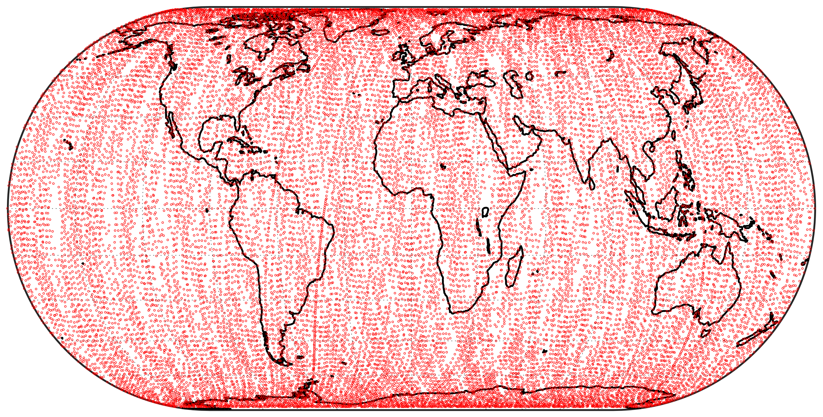
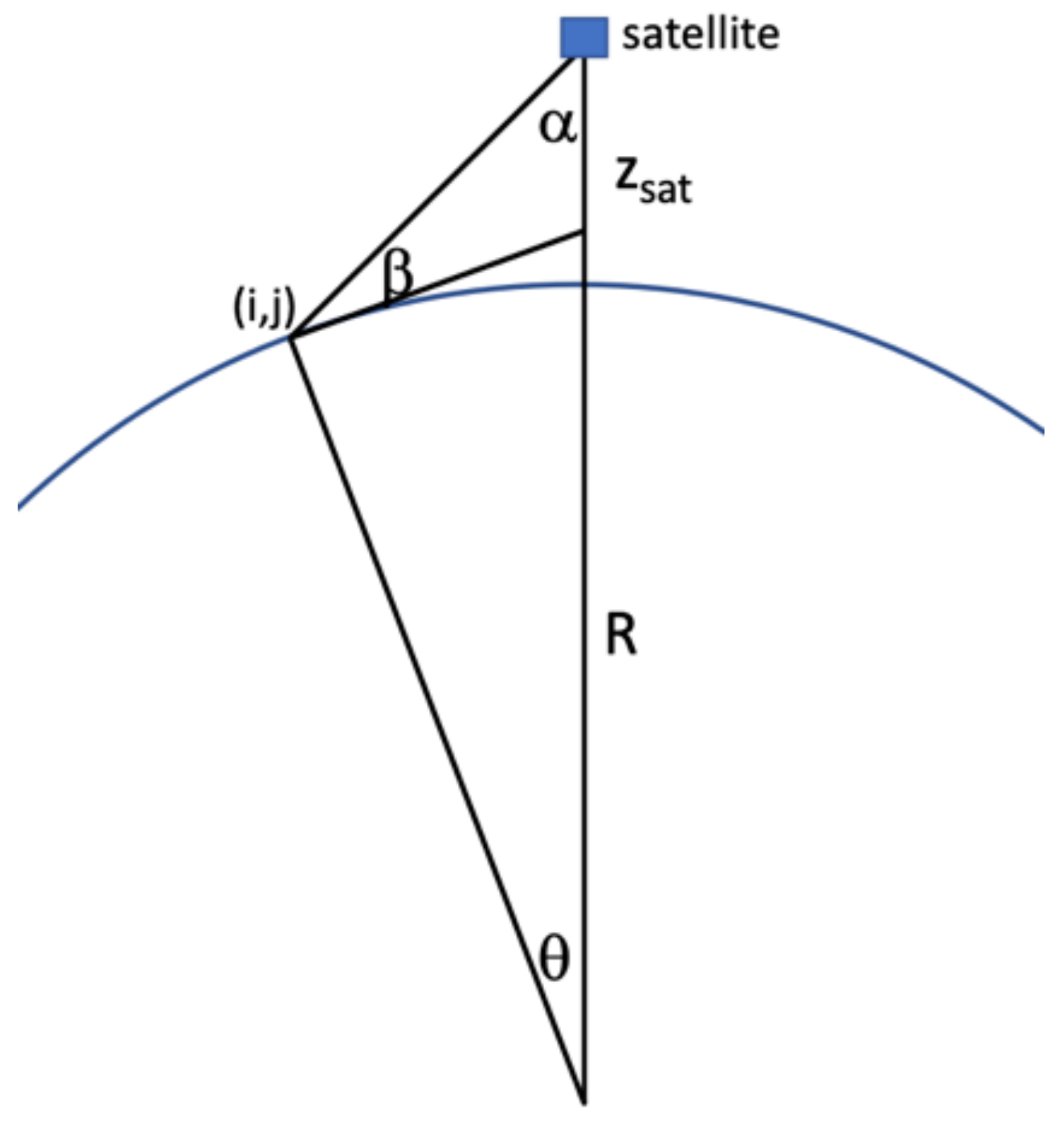
3.1.3. Methodology for Obtaining UVSQ-SAT Attitude and Position Time Series
3.2. Map Reconstruction Method from UVSQ-SAT Observation Time Series
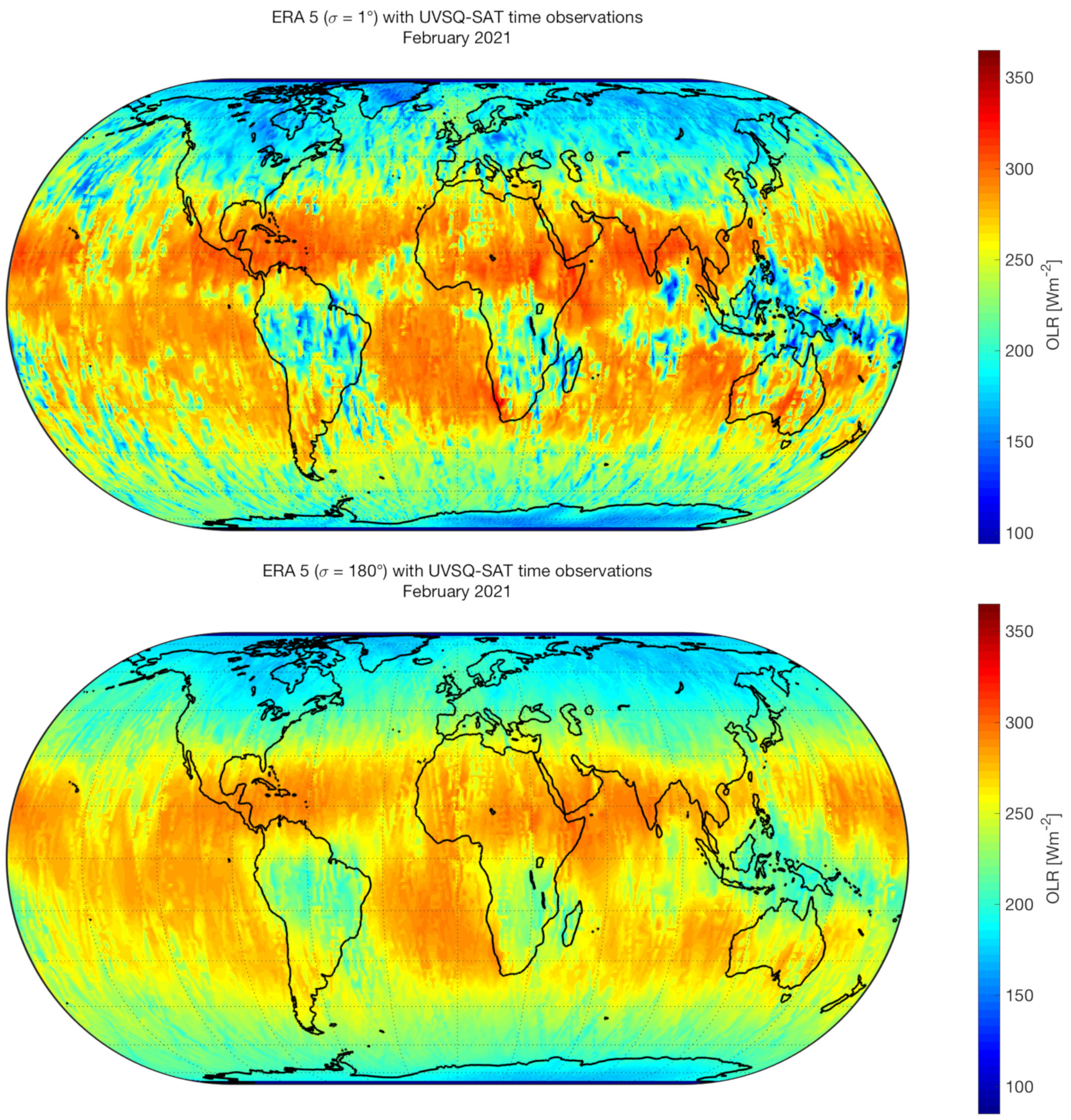
3.3. Reconstruction Method of the ERA 5 Maps to Compare with the UVSQ-SAT Maps
4. UVSQ-SAT First Observations
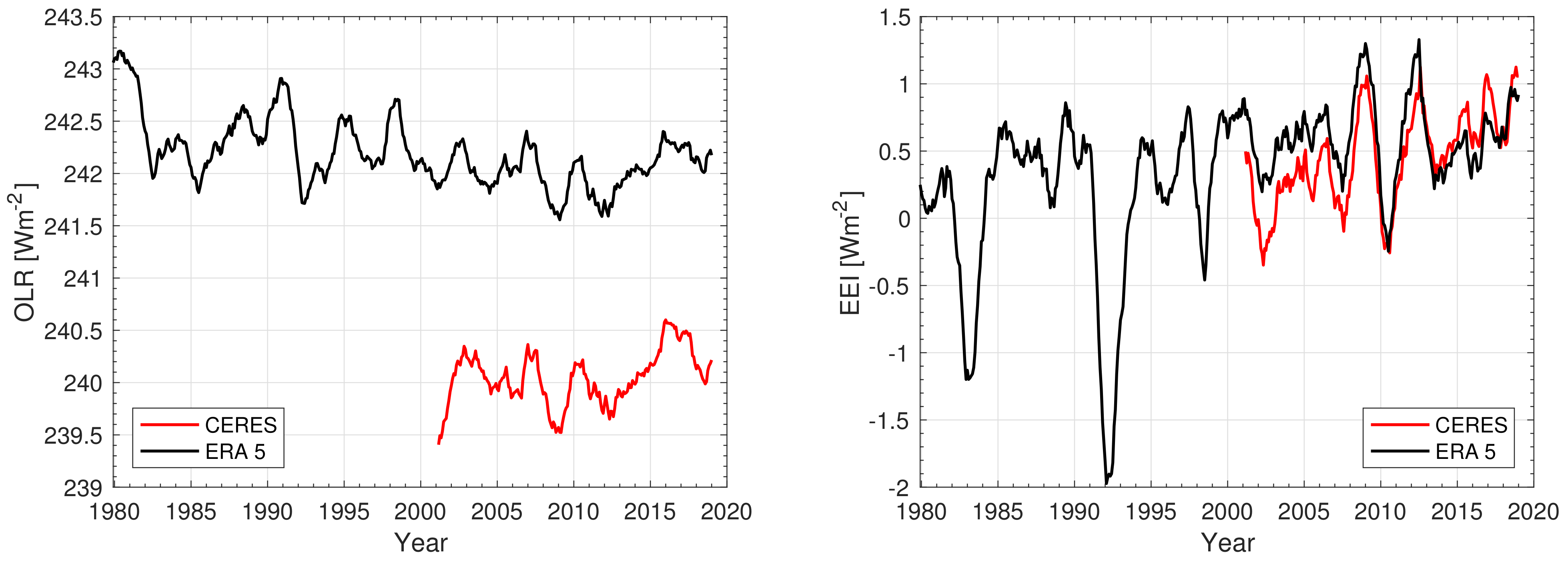
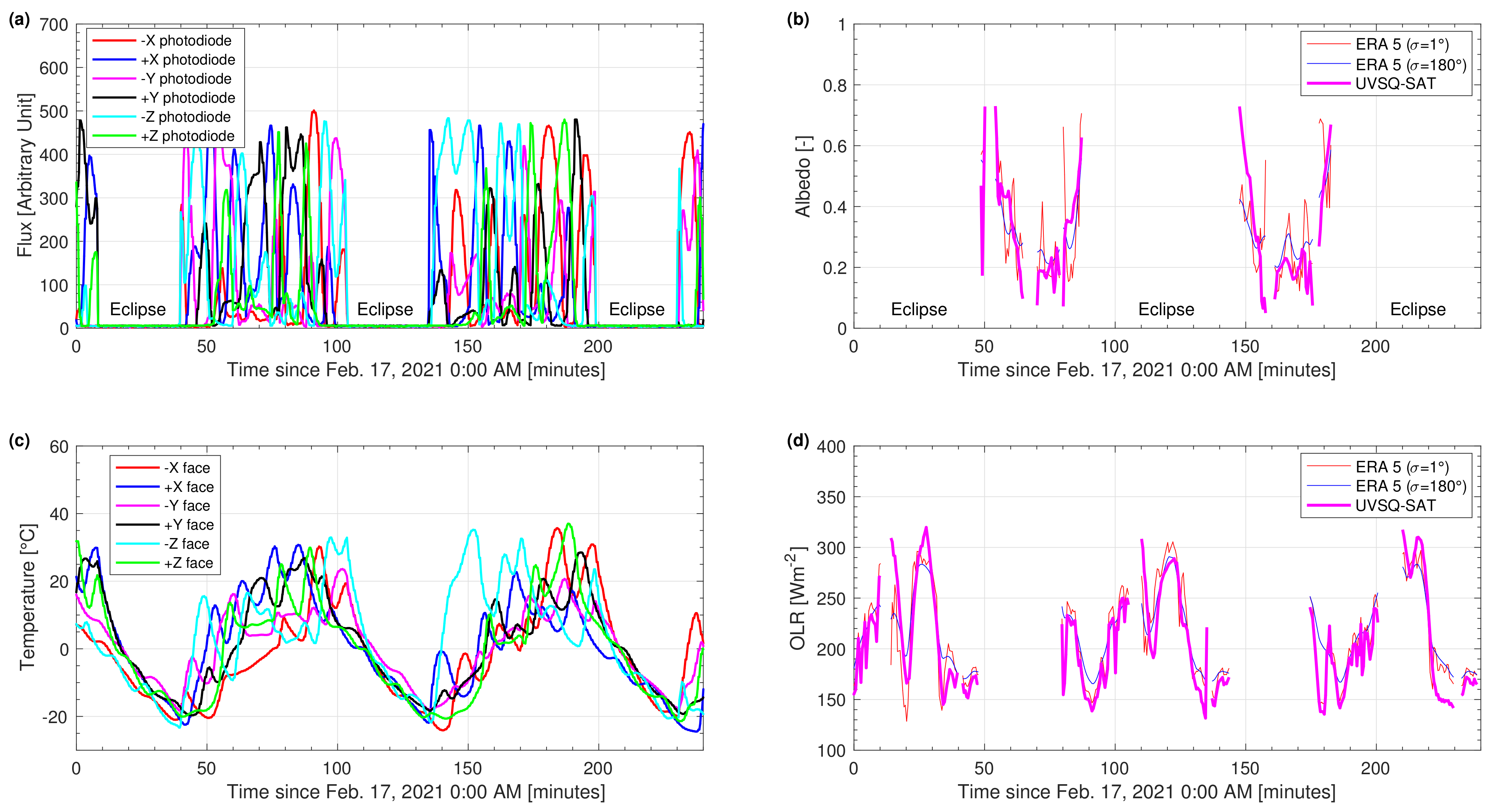
4.1. UVSQ-SAT Time Series
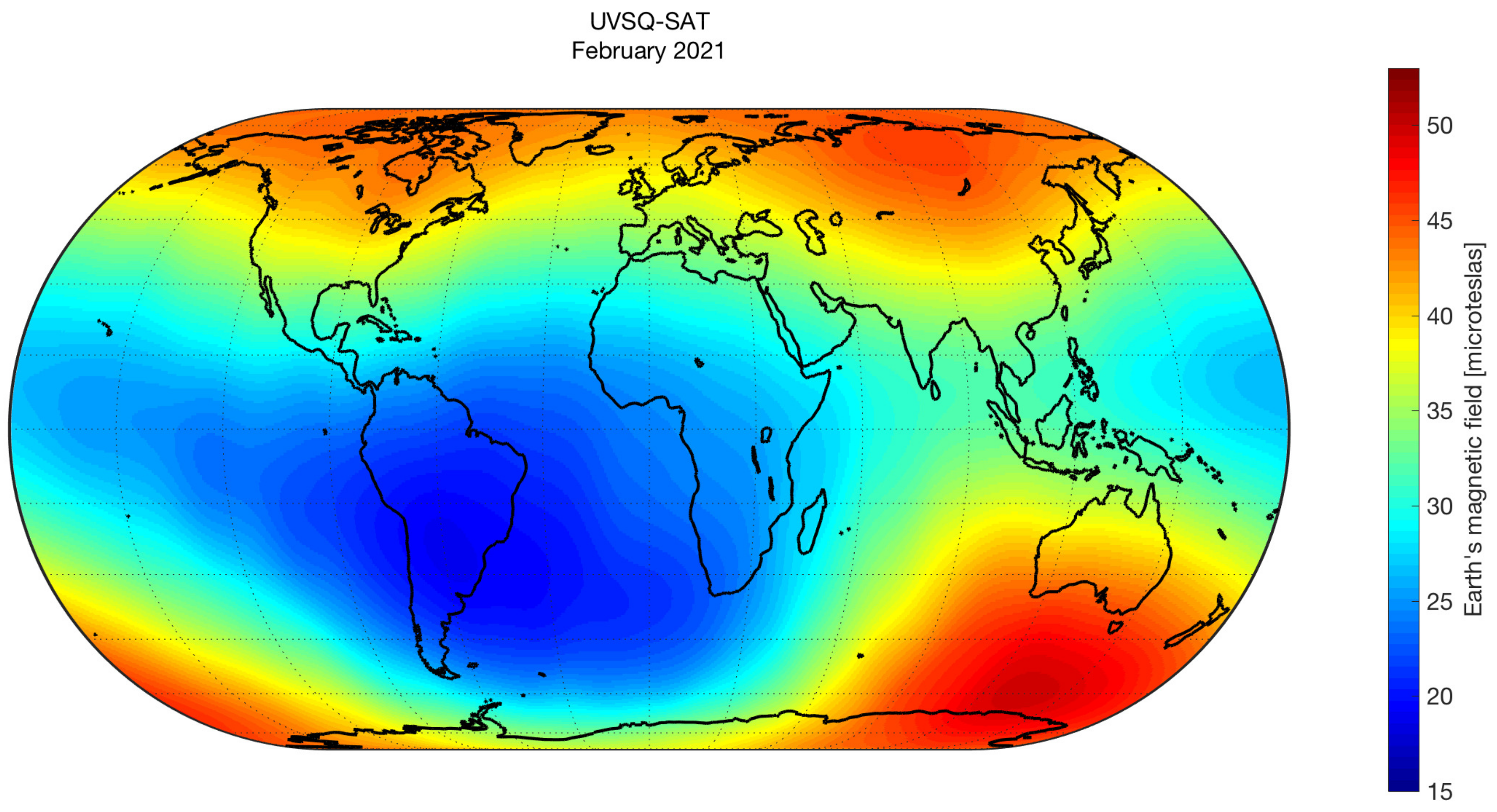
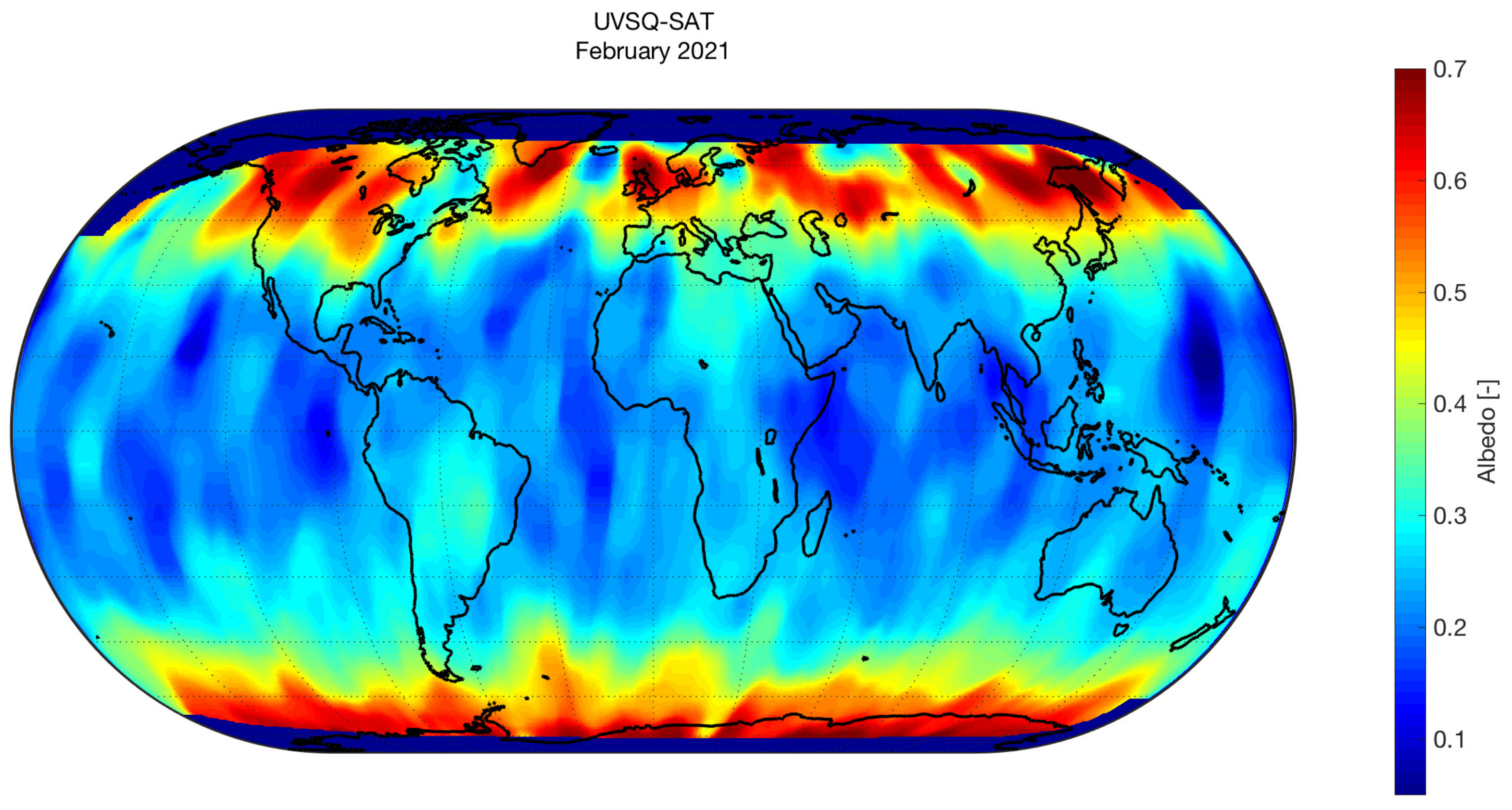
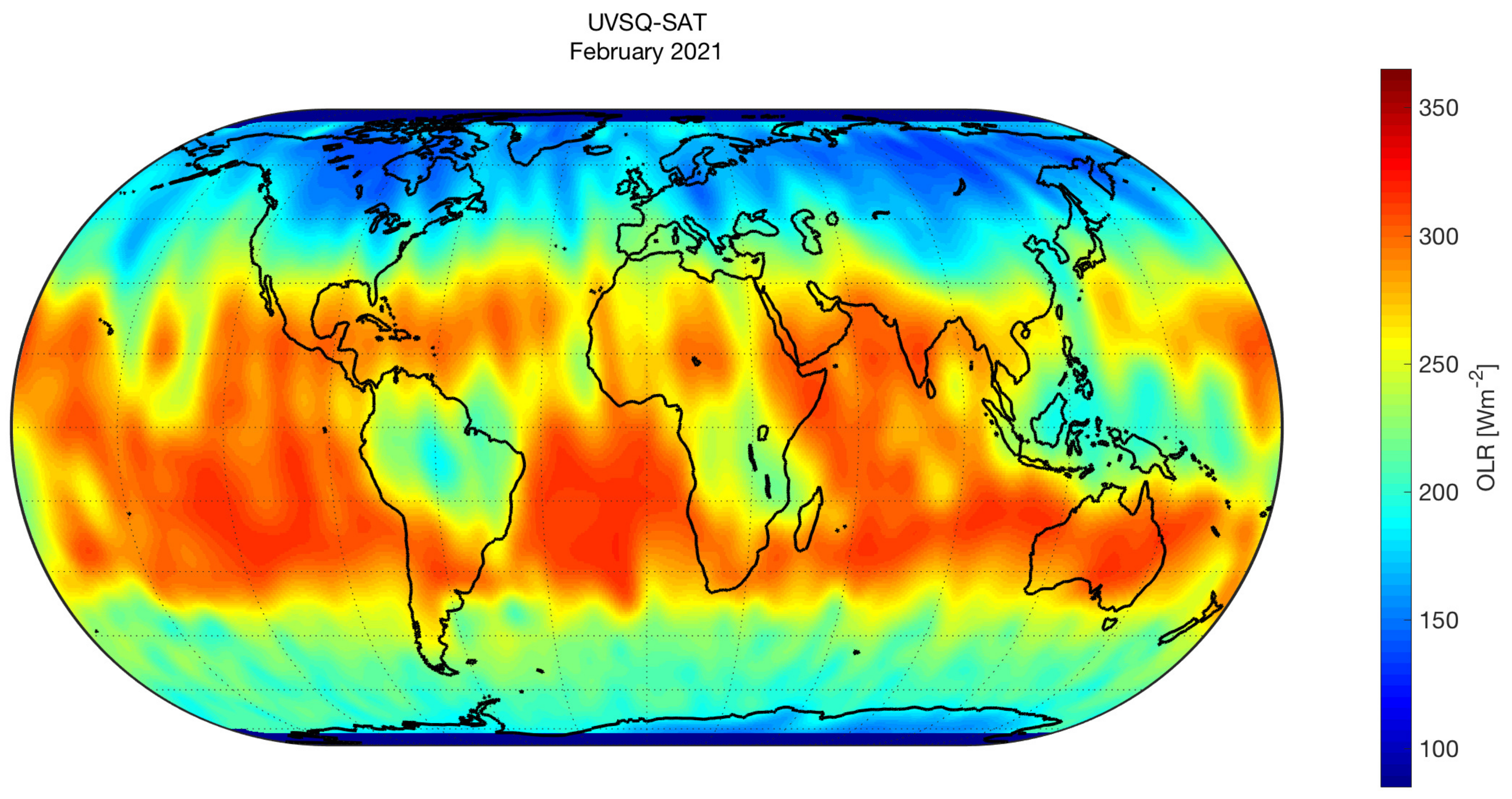
4.2. UVSQ-SAT Maps Reconstruction
5. Perspectives—Toward a Satellites Constellation for Climate Studies
6. Conclusions
Author Contributions
Funding
Acknowledgments
Conflicts of Interest
References
- Meftah, M.; Damé, L.; Keckhut, P.; Bekki, S.; Sarkissian, A.; Hauchecorne, A.; Bertran, E.; Carta, J.P.; Rogers, D.; Abbaki, S.; et al. UVSQ-SAT, a pathfinder cubesat mission for observing essential climate variables. Remote Sens. 2020, 12, 92. [Google Scholar] [CrossRef] [Green Version]
- Twiggs, R.J. Space system developments at Stanford University: From launch experience of microsatellites to the proposed future use of picosatellites. In Proceedings of the Small Payloads in Space, San Diego, CA, USA, 7 November 2000; Horais, B.J., Twiggs, R.J., Eds.; Volume 4136, pp. 79–86. [Google Scholar] [CrossRef]
- Puig-Suari, J.; Schoos, J.; Turner, C.; Wagner, T.; Connolly, R.; Block, R.P. CubeSat developments at Cal Poly: The standard deployer and PolySat. In Proceedings of the Small Payloads in Space, San Diego, CA, USA, 7 November 2000; Horais, B.J., Twiggs, R.J., Eds.; 2000; Volume 4136, pp. 72–78. [Google Scholar] [CrossRef]
- Xie, S.P.; Kosaka, Y. What caused the global surface warming hiatus of 1998–2013? Curr. Clim. Chang. Rep. 2017, 3, 128–140. [Google Scholar] [CrossRef]
- Von Schuckmann, K.; Palmer, M.D.; Trenberth, K.E.; Cazenave, A.; Chambers, D.; Champollion, N.; Hansen, J.; Josey, S.A.; Loeb, N.; Mathieu, P.P.; et al. An imperative to monitor Earth’s energy imbalance. Nat. Clim. Chang. 2016, 6, 138–144. [Google Scholar] [CrossRef] [Green Version]
- Loeb, N.G.; Manalo-Smith, N.; Su, W.; Shankar, M.; Thomas, S. CERES top-of-atmosphere Earth radiation budget climate data record: Accounting for in-orbit changes in instrument calibration. Remote Sens. 2016, 8, 182. [Google Scholar] [CrossRef] [Green Version]
- Allan, R.P.; Liu, C.; Loeb, N.G.; Palmer, M.D.; Roberts, M.; Smith, D.; Vidale, P.L. Changes in global net radiative imbalance 1985–2012. Geophys. Res. Lett. 2014, 41, 5588–5597. [Google Scholar] [CrossRef] [PubMed]
- Trenberth, K.E.; Fasullo, J.T.; Von Schuckmann, K.; Cheng, L. Insights into Earth’s energy imbalance from multiple sources. J. Clim. 2016, 29, 7495–7505. [Google Scholar] [CrossRef]
- Boyer, T.; Domingues, C.M.; Good, S.A.; Johnson, G.C.; Lyman, J.M.; Ishii, M.; Gouretski, V.; Willis, J.K.; Antonov, J.; Wijffels, S.; et al. Sensitivity of global upper-ocean heat content estimates to mapping methods, XBT bias corrections, and baseline climatologies. J. Clim. 2016, 29, 4817–4842. [Google Scholar] [CrossRef]
- Cheng, L.; Trenberth, K.E.; Fasullo, J.; Boyer, T.; Abraham, J.; Zhu, J. Improved estimates of ocean heat content from 1960 to 2015. Sci. Adv. 2017, 3, e1601545. [Google Scholar] [CrossRef] [PubMed] [Green Version]
- Kiehl, J.T.; Trenberth, K.E. Earth’s annual global mean energy budget. Bull. Am. Meteorol. Soc. 1997, 78, 197–208. [Google Scholar] [CrossRef] [Green Version]
- Stephens, G.L.; Li, J.; Wild, M.; Clayson, C.A.; Loeb, N.; Kato, S.; L’Ecuyer, T.; Stackhouse, P.W.; Lebsock, M.; Andrews, T. An update on Earth’s energy balance in light of the latest global observations. Nat. Geosci. 2012, 5, 691–696. [Google Scholar] [CrossRef]
- Trenberth, K.E.; Fasullo, J.T. Tracking Earth’s Energy. Science 2010, 328, 316–317. [Google Scholar] [CrossRef] [PubMed]
- Hansen, J.; Sato, M.; Kharecha, P.; von Schuckmann, K. Earth’s energy imbalance and implications. Atmos. Chem. Phys. 2011, 11, 13421–13449. [Google Scholar] [CrossRef] [Green Version]
- Von Schuckmann, K.; Cheng, L.; Palmer, M.D.; Hansen, J.; Tassone, C.; Aich, V.; Adusumilli, S.; Beltrami, H.; Boyer, T.; Cuesta-Valero, F.J.; et al. Heat stored in the Earth system: Where does the energy go? Earth Syst. Sci. Data 2020, 12, 2013–2041. [Google Scholar] [CrossRef]
- Pachauri, R.K.; Allen, M.R.; Barros, V.R.; Broome, J.; Cramer, W.; Christ, R.; Church, J.A.; Clarke, L.; Dahe, Q.; Dasgupta, P.; et al. Climate Change 2014: Synthesis Report. Contribution of Working Groups I, II and III to the Fifth Assessment Report of the INTERGOVERNMENTAL Panel on CLIMATE CHANGE; IPCC: Geneva, Switzerland, 2014. [Google Scholar]
- Gristey, J.J.; Chiu, J.C.; Gurney, R.J.; Han, S.C.; Morcrette, C.J. Determination of global Earth outgoing radiation at high temporal resolution using a theoretical constellation of satellites. J. Geophys. Res. Atmos. 2017, 122. [Google Scholar] [CrossRef]
- Finance, A.; Meftah, M.; Dufour, C.; Boutéraon, T.; Bekki, S.; Hauchecorne, A.; Keckhut, P.; Sarkissian, A.; Damé, L.; Mangin, A. A New Method Based on a Multilayer Perceptron Network to Determine In-Orbit Satellite Attitude for Spacecrafts without Active ADCS Like UVSQ-SAT. Remote Sens. 2021, 13, 1185. [Google Scholar] [CrossRef]
- Swartz, W.; Lorentz, S.; Papadakis, S.; Huang, P.; Smith, A.; Deglau, D.; Yu, Y.; Reilly, S.; Reilly, N.; Anderson, D. RAVAN: CubeSat Demonstration for Multi-Point Earth Radiation Budget Measurements. Remote Sens. 2019, 11, 796. [Google Scholar] [CrossRef] [PubMed] [Green Version]
- Wiscombe, W.; Chiu, C. The next step in Earth radiation budget measurements. In AIP Conference Proceedings; American Institute of Physics: College Park, MD, USA, 2013; Volume 1531, pp. 648–651. [Google Scholar]
- Baker, D.N.; Chandran, A.; Chang, L.; Macdonald, M.; Meftah, M.; Millan, R.M.; Park, J.H.; Kumar, P.; Price, C.; von Steiger, R.; et al. An International Constellation of Small Spacecraft. Space Res. Today 2020, 208, 23–28. [Google Scholar] [CrossRef]


| Contributor/Imbalance | Acronym | Flux |
|---|---|---|
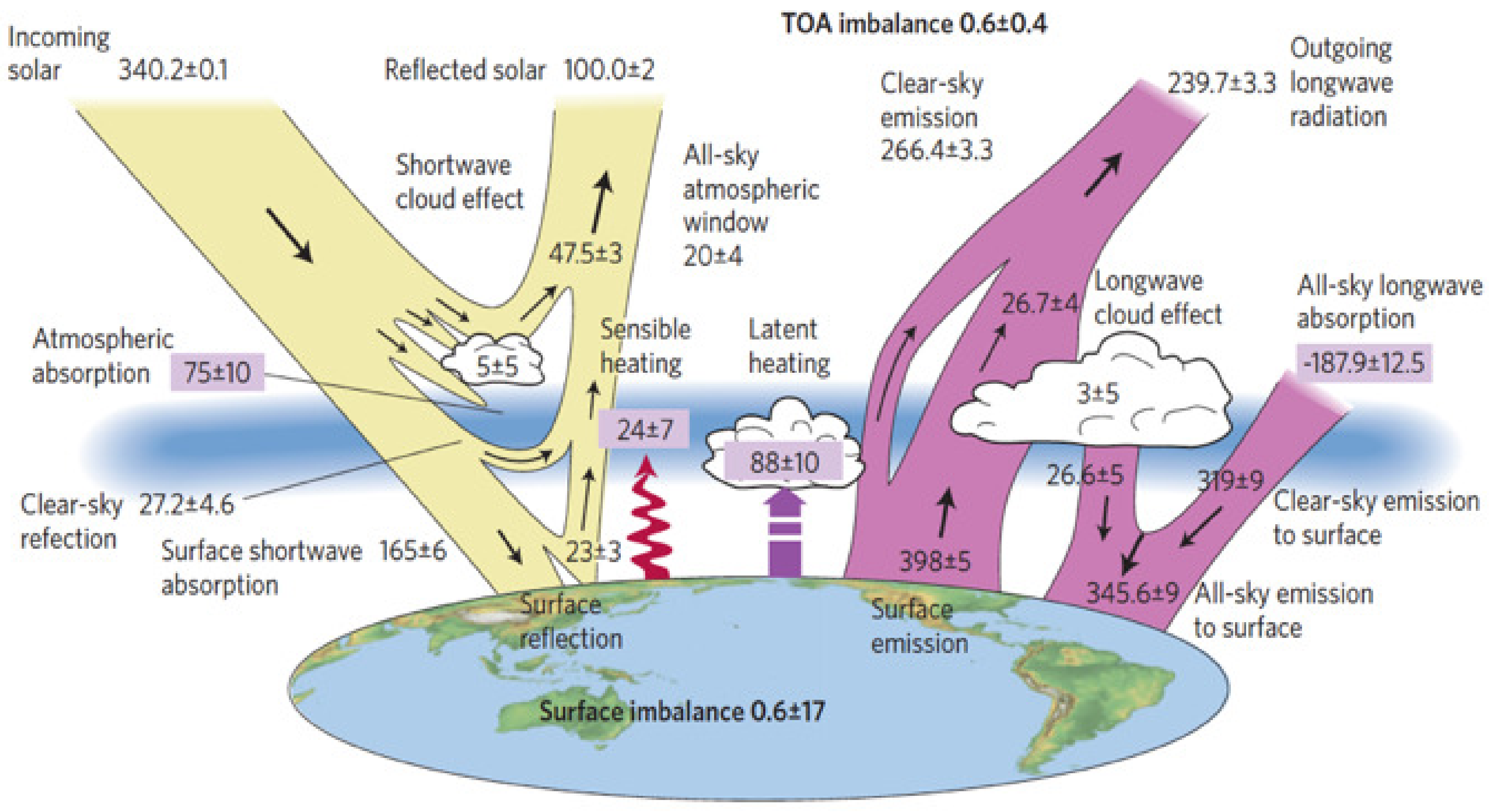
| Incoming solar radiation | TSI/4 | 340.2 ± 0.1 Wm |
| Outgoing shortwave radiation | OSR | 100.0 ± 2.0 Wm |
| Outgoing longwave radiation | OLR | 239.7 ± 3.3 Wm |
| TOA Earth energy imbalance | EEI at TOA | +0.6 ± 0.4 Wm |
| Surface Earth energy imbalance | EEI at surface | +0.6 ± 17.0 Wm |
| Requirements | Scientific Relevance | |||
| – | Absolute uncertainty | Stability per decade | Spatial resolution | Time resolution |
| TSI | ±0.54 Wm at 1 | ±0.14 Wm at 1 | – | 24 h |
| OSR | ±1.00 Wm at 1 | ±0.10 Wm at 1 | 10–100 km | Diurnal cycle |
| OLR | ±1.00 Wm at 1 | ±0.10 Wm at 1 | 10–100 km | Diurnal cycle |
| Requirements | UVSQ-SAT Performances | |||
| – | Absolute uncertainty | Stability per year | Spatial resolution | Time resolution |
| TSI | – | – | – | – |
| OSR | ±10 Wm at 1 | ±5 Wm at 1 | 1000 km | 15 days |
| OLR | ±10 Wm at 1 | ±1 Wm at 1 | 1000 km | 15 days |
Publisher’s Note: MDPI stays neutral with regard to jurisdictional claims in published maps and institutional affiliations. |
© 2021 by the authors. Licensee MDPI, Basel, Switzerland. This article is an open access article distributed under the terms and conditions of the Creative Commons Attribution (CC BY) license (https://creativecommons.org/licenses/by/4.0/).
Share and Cite
Meftah, M.; Boutéraon, T.; Dufour, C.; Hauchecorne, A.; Keckhut, P.; Finance, A.; Bekki, S.; Abbaki, S.; Bertran, E.; Damé, L.; et al. The UVSQ-SAT/INSPIRESat-5 CubeSat Mission: First In-Orbit Measurements of the Earth’s Outgoing Radiation. Remote Sens. 2021, 13, 1449. https://doi.org/10.3390/rs13081449
Meftah M, Boutéraon T, Dufour C, Hauchecorne A, Keckhut P, Finance A, Bekki S, Abbaki S, Bertran E, Damé L, et al. The UVSQ-SAT/INSPIRESat-5 CubeSat Mission: First In-Orbit Measurements of the Earth’s Outgoing Radiation. Remote Sensing. 2021; 13(8):1449. https://doi.org/10.3390/rs13081449
Chicago/Turabian StyleMeftah, Mustapha, Thomas Boutéraon, Christophe Dufour, Alain Hauchecorne, Philippe Keckhut, Adrien Finance, Slimane Bekki, Sadok Abbaki, Emmanuel Bertran, Luc Damé, and et al. 2021. "The UVSQ-SAT/INSPIRESat-5 CubeSat Mission: First In-Orbit Measurements of the Earth’s Outgoing Radiation" Remote Sensing 13, no. 8: 1449. https://doi.org/10.3390/rs13081449