Article

Uncertainty Estimation for Deep Learning-Based Segmentation of Roads in Synthetic Aperture Radar Imagery

1
Synthetic Aperture Radar Lab (SARlab), School of Engineering Science, Simon Fraser University, Burnaby, BC V5A 1S6, Canada
2
Digitalist Canada Ltd., Vancouver, BC V6B 4R3, Canada
*
Author to whom correspondence should be addressed.
Remote Sens. 2021, 13(8), 1472; https://doi.org/10.3390/rs13081472
Submission received: 12 March 2021 / Revised: 29 March 2021 / Accepted: 6 April 2021 / Published: 11 April 2021
(This article belongs to the Section Remote Sensing Image Processing)

Abstract

:
Mission-critical applications that rely on deep learning (DL) for automation suffer because DL models struggle to provide reliable indicators of failure. Reliable failure prediction can greatly improve the efficiency of a system, because it becomes easier to predict when human intervention is required. DL-based systems thus stand to benefit greatly from robust measures of uncertainty over model predictions. Monte Carlo dropout (MCD), a Bayesian method, and deep ensembles (DE) have emerged as two of the most popular and competitive ways to perform uncertainty estimation. Although literature exploring the usefulness of these approaches exists in medical imaging, robotics and autonomous driving domains, it is scarce to non-existent for remote sensing, and in particular, synthetic aperture radar (SAR) applications. To close this gap, we have created a deep learning model for road extraction (hereafter referred to as segmentation) in SAR and use it to compare standard model outputs against the aforementioned most popular methods for uncertainty estimation, MCD and DE. We demonstrate that these methods are not effective as an indicator of segmentation quality when measuring uncertainty (as indicated by model softmax outputs) across an entire image but are effective when uncertainty is measured from the set of road predictions only. Furthermore, we show a marked improvement in the correlation between prediction uncertainty and segmentation quality when we increase the set of road predictions by including predictions with lower softmax scores. We demonstrate the efficacy of our application of MCD and DE methods with an experimental design that measures performance in real-world quality assessment using in-distribution (ID) and out-of-distribution (OOD) data. These results inform the development of mission-critical deep learning systems in remote sensing. Tasks in medical image analysis that have a similar morphology to road structures, such as blood vessel segmentation, can also benefit from our findings.

Graphical Abstract

1. Introduction

1.1. Overview

Despite the enormous power of deep learning (DL) models, they are notoriously opaque. Mission critical domains such as autonomous driving, medical imaging, robotics and geospatial analysis all benefit greatly from the power of deep learning, but application and growth of DL in these areas is seriously hindered by models unable to identify failure modes reliably; models “do not know what they do not know” [1,2,3,4,5,6].
For example, we may wish to automate large-scale mapping of road structures in parts of the world undergoing rapid urban expansion so that emergency services can quickly reach these new areas via digital navigation applications. Deep learning systems can be trained to automatically extract roads from satellite images and do so much faster than any manual process.
However, a robust DL system must be able to manage inevitable quality problems. Models must indicate when their predictions are likely incorrect, or at least be able to flag inputs that the model has not been trained to deal with. Imagine that the road extraction model in the above example accidently received an image from a different distribution: an image processed with a different type of speckle filter or from a different sensor mode. In both of these cases, the model would have no reliable way of indicating that a problem has occurred. Moreover, production systems often experience dataset shift, which arises when subtle changes to data over time result in models being asked to make predictions over a slightly different distribution than that used for training [7]. This violates a basic assumption about DL models—that they are trained and tested on a single independently and identically distributed (IID) dataset—and means that resultant model behaviour is undefined. Other factors can also contribute to model uncertainty in the geospatial domain: labelling inaccuracies, a shortage of data over a particular terrain type, subtle differences in image preprocessing, differing weather conditions or image acquisition modes are a few examples. Ideally, estimation of uncertainty arising from these factors is reliable and clear so that systems flag images they cannot handle, human oversight is minimal and the benefits of automation are harvested in full.
Uncertainty estimation in deep learning is an open problem. Although the outputs of standard segmentation models are pushed through a softmax function to produce confidence scores over classes, it is well known that such confidence scores are miscalibrated, i.e., prone to overconfidence or underconfidence, even when the classifications are correct [1,8]. Additionally, the model outputs for each pixel are single deterministic class values (point estimates), which do not permit broader reasoning about uncertainty.
Various solutions have been proposed. One is to perform a post-hoc re-calibration of the model’s softmax outputs [1]. This is essentially a function that scales network outputs such that the predicted probability of each class matches the accuracy rate of each class. A limitation here is that calibration occurs with respect to in-distribution (ID) data, and this does not account for dataset shift or out-of-distribution (OOD) examples [7]. Another option is to use a generative model as a density estimator. Autoregressive models, for example, offer an exact marginal likelihood over data. Unfortunately, in practice, this approach does not yet work well [9]. Alternatively, Bayesian deep learning (BDL) methods can provide uncertainty estimates via a predictive distribution instead of the simple softmax point estimates afforded by deterministic models [3,7]. The caveat is that, due to the size and complexity of neural networks, BDL is not tractable without approximations to the posterior. Most approximations involve sampling techniques (e.g., Markov Chain Monte Carlo) or variational inference schemes [2,10,11]. Finally, although not technically Bayesian, DEs (training multiple similar networks and sampling predictions from each) have been proposed as a competitive strategy for obtaining uncertainty information [12].
Summary of Contributions: In this paper, we investigate the effectiveness of BDL methods for uncertainty measurement in automated road extraction from SAR images. We highlight the usefulness of SAR imagery for road extraction as an alternative to using optical imagery, as SAR is not subject to the same limitations (e.g., fog, nighttime) that optical sensors are. In doing so, we present a unique variation of the popular DeepLab model [13] that is a simple and effective way to segment roads. We assess uncertainty measurement methods on both ID and OOD samples using an experimental design that reflects real-world quality control performance. This allows us to explore the usefulness of uncertainty methods in “regular” data as well as robustness under dataset shift—specifically dataset shift under a typical SAR preprocessing variable: the presence of speckle. We emphasize that our goal is not to measure segmentation performance—which can vary substantially based on the preprocessing techniques or SAR sensor types used to construct a dataset—but to measure uncertainty performance, which should remain reasonably stable across differences in datasets. Importantly, we demonstrate that measuring uncertainty over all image pixels is not effective, and we significantly increase quality assessment performance by measuring uncertainty over road predictions using a low initial decision threshold. To the best of our knowledge, this is the first time this simple technique, which is different than recalibration, has been used in the literature in this way to increase the usefulness of softmax scores for uncertainty estimation. We also present the surprising result that none of the metrics proposed to reason about distributions of samples from a stochastic model’s softmax outputs (e.g., variance, mutual information, Kwon et al.’s aleatoric or epistemic uncertainty [14]) provide more useful information than Bayesian model averages (BMA). Finally, we add to existing evidence that DEs provide more useful uncertainty information than the popular MCD method, though DEs still struggle to approximate the predictive posterior distribution.

1.2. Prior Work

Prior to operational DL methods, road extraction in SAR images used classical models that were constructed with hand-picked features such as geometry, radiometry and topology [15,16,17]. The basic idea was to craft knowledge of road-specific characteristics, e.g., linearity, height relative to surroundings, surface characteristics etc. into the model a priori. As feature rules could vary based on region or sensor type, models relied on the fusion of feature and image sets to improve generalization [16,18]. Some approaches utilized a Bayesian framework to reason about distributions of features in different contexts [19,20,21]. The challenge with these initial approaches was that even ostensibly simple a priori knowledge is extremely complex and difficult to encode in a model. For example, it is true that roads are generally “linear”, but across suburbs, highways and ocean sides they have complex geometries (width, degree of curvature, widely varying lengths) that make codification into a ruleset difficult or impossible.
Supervised learning methods such as conditional random fields and support vector machines alleviated these issues somewhat by learning parameters over features, so that knowledge did not have to be encoded as explicitly [22,23,24]. However, features still needed to be crafted prior to ingestion into the model (e.g., with Gabor filters), so that the information over which the model “learned” was tractable. So, while the complexity of explicit encoding within the model was reduced, the question of which features to use remained unanswered.
Deep learning addresses this issue. With minimal preprocessing of data, a DL model is capable of learning which features are best for the task the model is trained on [25]. To the best of our knowledge, no extensive performance comparison between classical, early machine learning (ML) and DL models has been conducted for SAR applications. However, DL methods applied to image segmentation and classification tasks have produced far superior results to earlier methods across a variety of computer vision applications [26,27,28], and we have no reason to believe SAR segmentation applications would behave differently.
Recently, work on DL-based road extraction in SAR remote sensing images includes Zhang et al. using a U-Net to extract roads from Sentinel-1 data (10 m × 10 m per pixel resolution) with good results [29]. Similarly, Henry et al. explore road extraction in TerraSAR-X imagery (1.25 m × 1.25 m resolution) using a U-Net and DeepLab, and find the latter to be superior [30]. Both methods use speckle filtering techniques to preprocess the data.
Nearly all applications of Bayesian deep learning (BDL) methods in the literature arise in medical imaging or autonomous driving domains [5,6]. Only one paper has explored BDL in the SAR domain [31]. However, this paper only achieves a maximum a posteriori (MAP) point estimate of uncertainty, as their generative adversarial network (GAN)-based approach is deterministic: it takes a previous network’s outputs as its inputs, as opposed to the Gaussian noise that a standard GAN receives. Furthermore, although several DL methods for uncertainty measurement and calibration have been published [1,2,10,11,12,32,33], evaluations of the utility of these uncertainty measurements in real-world scenarios are sparse [5,14,34,35,36] and are non-existent in SAR literature.
Comparing the effectiveness of BDL methods across domains, tasks and datasets is a large task far beyond the scope of the present study, which instead is motivated specifically by the paucity of BDL research in SAR. Concretely, our paper aims to demonstrate the effectiveness of BDL for the SAR road extraction task. Beyond the specific focus of the paper, we hope to contribute to an emerging consensus on the effectiveness of BDL techniques generally as a starting point to use BDL in novel contexts for other applications, especially in the remote sensing domain.

2. Materials and Methods

2.1. Dataset

We are not aware of a publicly available SAR dataset specific to road segmentation, so we created one from RADARSAT-2 (R2) data. The data used for all experiments is a 15-image stack of 18,000 km2 swaths of R2 SGF, extra-fine imagery over the San Francisco Bay Area. Images were acquired from 21 July 2014 to 7 March 2017. RADARSAT-2’s SGF extra fine mode has a nominal ground resolution of approximately 5m. Images have HH polarization and are right-looking with a mid-image incidence angle of 41 degrees.
All 15 raw SAR images were coregistered to better than 1/10 of a full-resolution pixel, and then converted from the native 16bit unsigned integer to lossless 32bit floating point TIFF images. Multi-temporal filtering (MTF) across all images was used to remove speckle noise and improve the quality of the segmentation results [30]. Ground truth labels were created from OpenStreetMap data. The data were geocoded and projected to match the SAR image and converted to a binary raster image using GDAL.
A histogram analysis of SAR images revealed that most information is concentrated between floating point values of 0 and 0.1, with a very long tail. Clipping the data at 0.3 improved numerical stability during training, while including the majority of sensor information.
The processed SAR image and accompanying label image was then cut into 2012 512 px × 512 px image “chip” pairs, with 402 image chips (20%) reserved for testing. As the most time-consuming portion of a real-world system would involve quality checking complex road structures in developed areas, we withdraw test image chips that do not contain roads, e.g., areas over water. Since we do not have access to the unfiltered, raw SAR images, we chose to create an OOD dataset using a function to re-introduce SAR amplitude speckle with the corresponding MTF image chips serving as the underlying backscatter maps. Each MTF image chip thus has a speckled counterpart. The result is a new test set that is exactly twice the size of the ID set, composed of speckled and filtered image chips. We consciously chose this approach as appropriate for the SAR case over alternate distortions that arise in optical sensors (and accompanying benchmarks), such as defocus blur or changes in brightness and contrast [37]. The speckle simulation function is:
S   =   I [ 0.5 0.5 ( F 2 + G 2 ) 0.5 ]  
where S is the resultant speckled image chip, I is the MTF SAR image chip, ⊙ represents the Hadamard product, and F,G are chip-sized 512 × 512 matrices with elements independently random-sampled from a standard Gaussian distribution. Example image chips are shown in Figure 1b. Prior to model ingestion, all image chips were randomly augmented with horizontal or vertical flips, and 90-degree rotations.
Some final notes on the limitations of this dataset should be mentioned. The labels created from OpenStreetMap contain an unavoidable level of noise. This is due to three factors: the OpenStreetMap data did not perfectly match the actual widths of roads, the filtered SAR images spanned approximately 2.75 years and thus some roads were presumably built/changed in that time, and there are likely also errors present in the OpenStreetMap road data itself. Additionally, our particular SAR sensor data and preprocessing methods have been chosen to create high signal-to-noise ratio data ideal for road segmentation. As such, our data quality approximates that which would be used in a real-world, production quality system. Using data from a different sensor (especially with a lower SNR), choosing different imaging or preprocessing methods, an increased number of image artifacts (foreshortening, motion errors [38]) or having perfect labels would alter the quality of the segmentation model. However, our aim is not to deliver state-of-the-art segmentation results, nor to determine the optimal image specifications required to perform road segmentation. Instead, we provide an experimental framework to assess the usefulness of uncertainty measurement methods in a real-world system. With this in mind, it is our contention that sources of error in the labels or the presence of image artifacts are a feature, not a bug, as these reflect real-world conditions and emphasize the utility of uncertainty measures. This said, an ideal dataset would contain numerous sensor types, imaging methods, etc., in order to precisely examine the generalizability of these methods to any context, since no such formal guarantees exist in DL yet. Constructing a dataset to exhaustively meet these empirical demands, although an excellent topic for future research, would be very expensive and is beyond the scope of this study. However, our results across ID and OOD datasets provide evidence that uncertainty methods generalize reasonably well, despite our expectation that segmentation performance will fluctuate significantly across models and datasets (see Section 3 for more details).

2.2. Segmentation Model

It is generally accepted that convolutional neural networks (CNN) are the method of choice for image segmentation problems. We define image segmentation given input image X, a corresponding ground truth binary map Y of size XHeight·XWidth indicating the presence or absence of a road at each pixel, and the output of the model Y ^ of size XHeight·XWidth·2, which contains a softmax probability over the road/no-road classes. To test the model’s output with the ground truth label, we select the larger softmax probability for each pixel and are then left with a binary map that can be directly compared with ground truth.
Two of the most common model choices for image segmentation problems are U-Net and DeepLab [13,39]. We found experimentally that our adapted DeepLab model was superior to a U-Net configuration (Figure 2), and therefore use DeepLab for all of our experiments. DeepLab is composed of a ResNet backbone and an Atrous Spatial Pyramid Pooling (ASPP) block. As roads in SAR images can occupy as little as 4–6 px in width, the standard receptive field sizes of a ResNet (at least 16 px) are too large to detect them. We reduce downsampling to produce a receptive field size of 4px at the output of the ResNet backbone. These embeddings are fed into the ASPP block and upsampled to produce class predictions for each pixel in the image, as per the standard DeepLab architecture. Although less downsampling reduces the so-called “information bottleneck”, there is evidence to suggest that bottlenecking is not as essential to learning in deep models as previously thought [40]. The strong performance of our network supports this idea empirically. We believe it may not always be necessary to have more complex architectures that include bottleneck structures with skip connections (e.g., U-Net, DeepLab3+) such as are used to recover higher-detail information after the downsampling process.

2.3. Uncertainty in Deep Learning

Although the softmax output of a segmentation model resembles a probability distribution over class predictions, this does not necessarily provide an unbiased and accurate measure of uncertainty. Models are often incorrect with high confidence [1,6]. Models also lack awareness of whether a given input is from the distribution they were trained on. A model trained on speckle filtered SAR images would not be well-equipped to predict results on speckled SAR images. The uncertainty from an OOD input may not be evident in the result, meaning the model confidently makes predictions on data it knows nothing about.
In addition to these limitations, a softmax output from a single deterministic model provides only a point estimate of uncertainty. In contrast, Bayesian methods [41] provide a posterior over model parameters given the data:
p ( ω | X , Y ) = p ( Y | X , ω ) p ( ω ) p ( Y | X )
where X, Y is the set of all image chips and corresponding ground truth labels respectively, and ω is the set of model parameters. To produce a predictive distribution, we employ the posterior and model predictions, and integrate over model parameters [41]:
p ( y ^ | x , X , Y )   =     p ( y ^ | x   , ω ) p ( ω | X , Y ) d ω  
which permits, for a pixel x, a posterior-weighted average over model predictions y ^ , also known as a Bayesian model average. The difficulty here is that deep learning models have too many parameters to allow an analytical solution for the posterior. This is due to the marginal likelihood term from Equation (2):
p ( Y |   X )   =     p ( Y |   X , ω ) p ( ω ) d ω  
where ω has millions of parameters and so renders integration intractable. Bayesian deep learning thus seeks to approximate the posterior. Perhaps the most common way to do this in deep neural networks is to use Monte Carlo Dropout [2,3]. Dropout, which involves randomly dropping neurons from network layers during training, was originally motivated as a technique to prevent overfitting [42]. However, it can be shown that, when used with the proper minimization objective, dropout is analogous to variational inference [2].
Variational inference proposes an approximating distribution for the posterior, q θ ( ω ) = p ( ω | X , Y ) , and relies on a minimisation objective to shape the parameters θ of q θ ( ω ) , such that the two distributions are as similar as possible. The Kullback–Liebler divergence is used as a similarity metric, and minimizing this divergence is synonymous with maximizing the evidence lower bound. Our variational loss objective, L V I , becomes [2]:
L V I ( θ )   : =   q θ ( ω ) l o g p ( Y | X , ω ) d ω     K L ( q θ ( ω ) | | p ( ω ) )  
The first (likelihood) term can be interpreted as penalizing model inaccuracy, and the second (KL) term can be interpreted as enforcing similarity between the posterior and prior distributions. It can be shown that minimizing this objective is analogous to training a neural network with L2 regularization and a dropout scheme, which affords a mixture of Gaussians as approximation to the posterior [2].
Once the model is trained, leaving dropout enabled at prediction time can be interpreted as taking samples from the posterior. These samples approximate an integration over the predictive distribution, and averaging predictions results in our BMA [2]:
p ( y * | x * , X , Y )   p ( y * |   x * , ω ) q ( ω ) d ω   1 T t = 1 T p ( y * | x * , ω t )  
Other measures of uncertainty over our predictive distribution can be taken. Aleatoric uncertainty arises from noise in the data, e.g., label noise or sensor noise inherent in the acquisition process. Epistemic uncertainty originates from the model, which can include capacity, architecture or other such model parameters, as well as uncertainty due to a lack of data.
Kendal and Gal [6] proposed a method to decompose model outputs into aleatoric and epistemic measures of uncertainty. While their solution for the regression case is reasonable, the classification case (which interests us here) is potentially problematic [14]. Kwon et al. argue that Kendal and Gal’s method measures uncertainty only indirectly, i.e., over the linear outputs of the network (logits) rather than the post-softmax non-linear predictive distribution. Additionally, Kwon et al.’s measurement of the predictive distribution requires no additional parameters during training. We therefore investigate Kwon et al.’s proposed method:
1 T t = 1 T d i a g ( p t ^ ) p ^ t 2   +   1 T t = 1 T ( p ^ t p ¯   ) 2  
where p ¯ = t = 1 T p t ^ / T and p t ^ = S o f t m a x { f w ^ t ( x * ) } , the left side of the summation is aleatoric uncertainty, and the right side is epistemic uncertainty. Here, “epistemic” uncertainty is high when predictions vacillate confidently from one class to another, while “aleatoric” uncertainty is high when multiple class predictions are close to the decision threshold (e.g., 50% for a binary decision).
We can also measure the variance, entropy and mutual information over model outputs. Entropy is a measure of the information present in the predictive distribution [43]:
H [ y i * | x i * , X , Y ]     c = 1 C 1 T t = 1 T p ( y i * = c | x i * , ω t ) l o g ( 1 T t = 1 T p ( y i * = c | x i * , ω t ) )
where C is the number of classes, T is the number of samples from the model and ωt is the model weights at sample t. Mutual information is the difference of the entropy of the average model prediction and the expectation of entropy over each prediction [43]:
M I [ y i * , ω | x i * , X , Y ]   H [ y i * | x i * , X , Y ]   E [ H [ y i * | x i * , ω ] ]
This quantity differs from entropy in that it highlights cases where the model is confident in each prediction but vacillates between classes across predictions.
It is notable that MCD can be interpreted as averaging over an ensemble of networks with shared weights [42], and this has motivated investigation into ensembles without shared weights as a method of uncertainty measurement [12]. DEs can be created for this purpose by training the same architecture multiple times, with each training instance initialized by a unique set of random weights. At prediction time, the same data point is evaluated by each individual network and the results are averaged. Although this process is not Bayesian, it arguably results in a Bayesian model average [10], and the samples taken over multiple models can be measured with the same quantities noted above.
Recent research has demonstrated that DEs provide superior measures of uncertainty to non-ensembled Bayesian techniques such as MCD or SWAG [3,7,10]. It is speculated that this is because these latter methods sample weights in the neighbourhood of a single local minimum. Models in a DE each converge on unique local minima across the loss landscape, and this greater diversity of sampling regions is thought to produce a better predictive distribution [10,44]. However, this strategy carries the cost of longer training times and more overhead due to the management of several large models per inference pass.

2.4. Loss Function and Segmentation Metrics

Road pixels comprise a relatively small fraction of the dataset, compared to non-road pixels. The binary cross-entropy loss function is standard in classification tasks in ML [41], and is used in our segmentation task as well:
L C E =   v V p ( y v ) l o g p ( y ^ v )   + p ( 1 y v ) l o g p ( 1 y ^ v )
where V is the set of image pixels, y is the ground truth label for the pixel and y ^ is the corresponding model softmax output for that class, which considers each pixel’s class equally, and unless weighted to account for a class imbalance, generates much more loss from non-road pixels. Intersection over union (IoU, also known as Jaccard index [45]) shows up frequently in ML and provides a direct comparison of ground truth and predicted road areas, and thus accounts for the class imbalance. IoU is formulated as:
L I o U =   T P F P   +   T P   +   F N = I ( X ) U ( X )
where TP, FP and FN are the true positive, false positive and false negative counts of pixels in an image chip, respectively. In order to make this differentiable, we define I(X) and U(X) as [46]:
I ( X ) = v V X v Y v
U ( X ) = v V ( X v + Y v X v Y v )  
where V is the set of all pixels in an image chip, Xv is the probability of a road pixel at pixel v, and Yv is a one-hot encoding of the ground truth label at pixel v.
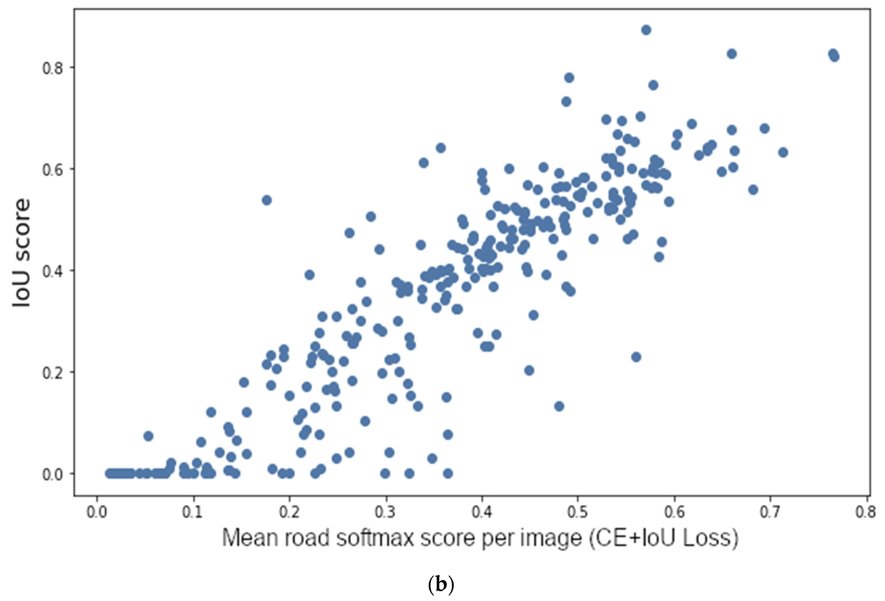
We observed experimentally that an objective function consisting of the sum of cross-entropy and IoU loss yielded the best test time results. Adding cross-entropy to the IoU loss also provided better calibration than IoU alone (Figure 3).
In addition to road morphology, which is measured by IoU, we also wish to assess road topology. Average path length score (APLS) has been proposed to measure this quality in road structures [47]:
A P L S   =   1     1 N n = 1 N m i n { 1 , | L ( a , b )     L ( a , b ) | L ( a , b ) }
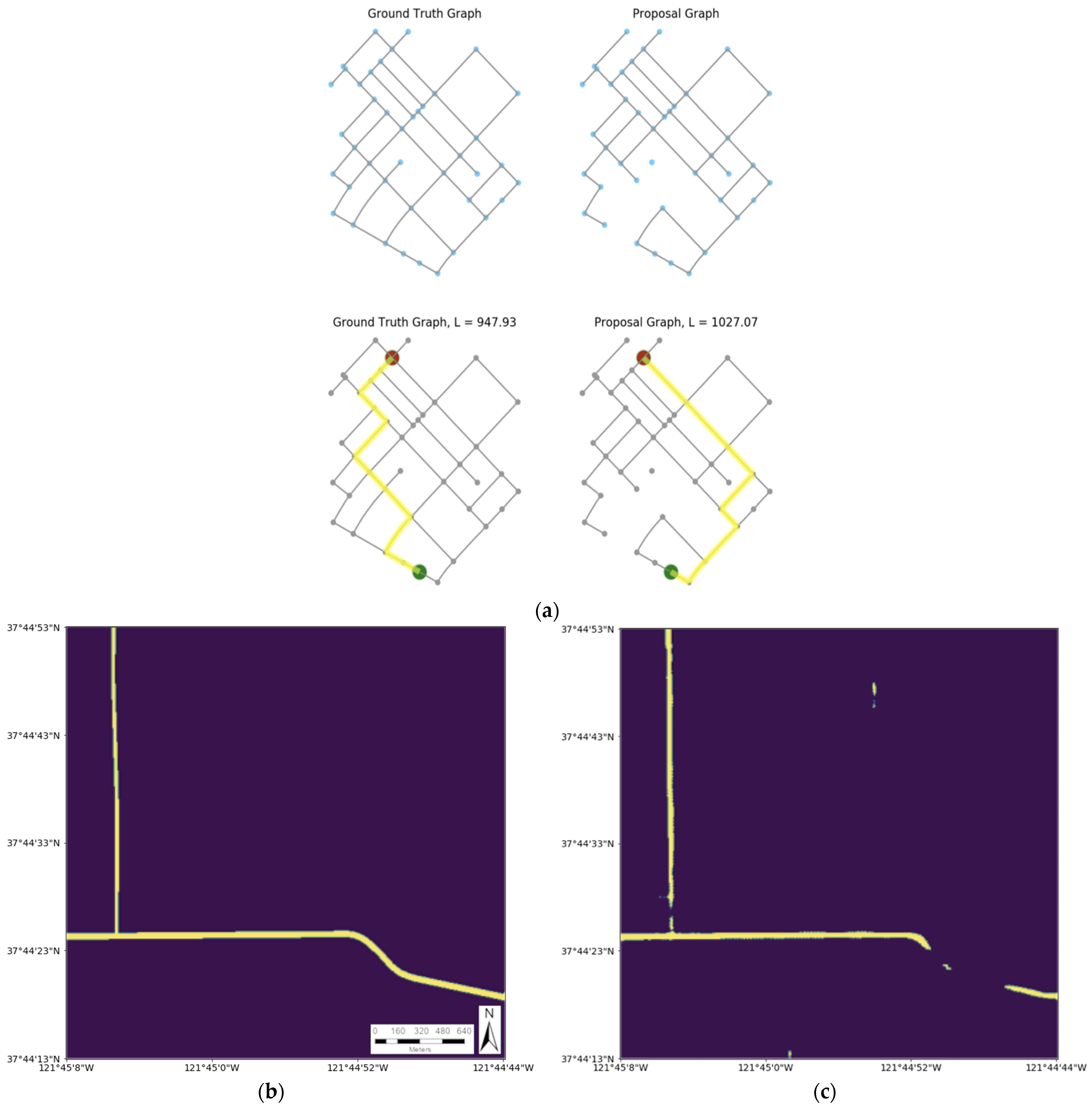
Here, we first take model predictions and transform them into graph representations (Figure 4a). In Equation (14), N is the total number of paths between all nodes in the graph, a,b represents start and end nodes of a path in the ground truth graph, a′,b′ are the closest corresponding nodes from the prediction graph, and L is a distance function. APLS is penalized both for adding edges (false positive road sections) that allow for shorter paths, and for excluding edges (false negatives) that create longer paths (see [47] for more details).
The motivation for this additional metric becomes clear when compared to IoU. IoU penalizes errors in the area of roads but does not heavily penalize connective mistakes (Figure 4b,c). Note that APLS is not differentiable with respect to model weights (due to transformations required to produce a graph from the segmented predictions output from the network) and cannot be used as a loss function.
To measure the real-world usefulness of uncertainty methods, we use an experimental design proposed by Leibig et al. [5]. Here, the p percent most uncertain image chips are excluded from testing scores. The idea is that the image chips the model reports as most uncertain are advanced for inspection and correction by humans. We then score the model only on image chips not advanced for inspection. If model uncertainty and segmentation quality are well correlated, model scores (as measured by IoU and APLS) increase as we send more image chips for inspection.
To allow us to analyze score improvements made by thresholding image chips separately from model performance, we propose a simple sum of uncertainty gains (SUG) metric, which is the sum of differences of scores of each percentage of retained data and the full test set:
C   =   m M k = 1 K D m 100 10 k D m 100
where D is the score of metric m in M = {IoU, APLS} with percentage 100 − 10k of the test data retained for scoring, and K is the number of thresholds at which we measure score improvement. For example, if one model performs worse than another on overall segmentation quality, but the underperforming model shows more improvement than the other when thresholding image chips for quality review, it will have a higher SUG score.

2.5. Improving Uncertainty Measurements

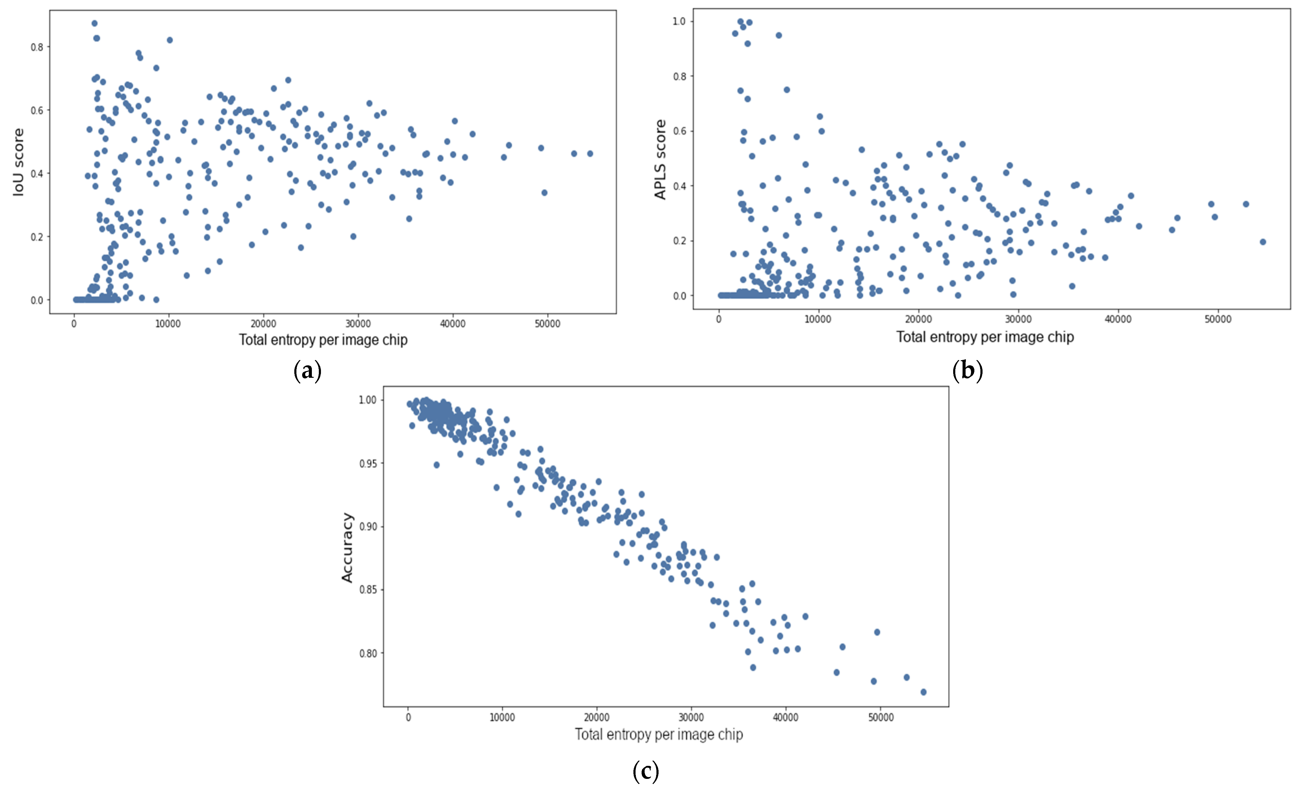
That relatively few image chip pixels are roads means that the uncertainty in a given image chip can be suppressed by a majority of very confident non-road pixels. This obscures a correlation between image chip uncertainty and segmentation quality. For example, although there is a strong correlation between entropy over all image chip pixels and pixel-wise segmentation accuracy (the percentage of correctly classified pixels in a chip), entropy measured in this manner does not correlate with IoU or APLS metrics (Figure 5).
This means that entropy over all pixels cannot be used to threshold poorly segmented image chips for quality inspection. To rectify this problem, we measure uncertainty only over road pixels, which is well correlated with our metrics of interest (Figure 3).
Intuitively, this makes sense: It is reasonable that the model would learn that roads tend not to have discontinuities. However, for various reasons—such as cul-de-sacs in suburbs, overhanging trees, and unusual surface variations—gaps do arise, and it is often these places that the model classifies pixels incorrectly. Measurement of uncertainty within these connective regions would increase the quality of the uncertainty for a given image chip, but it is difficult to reliably identify such areas in the absence of ground truth labels.
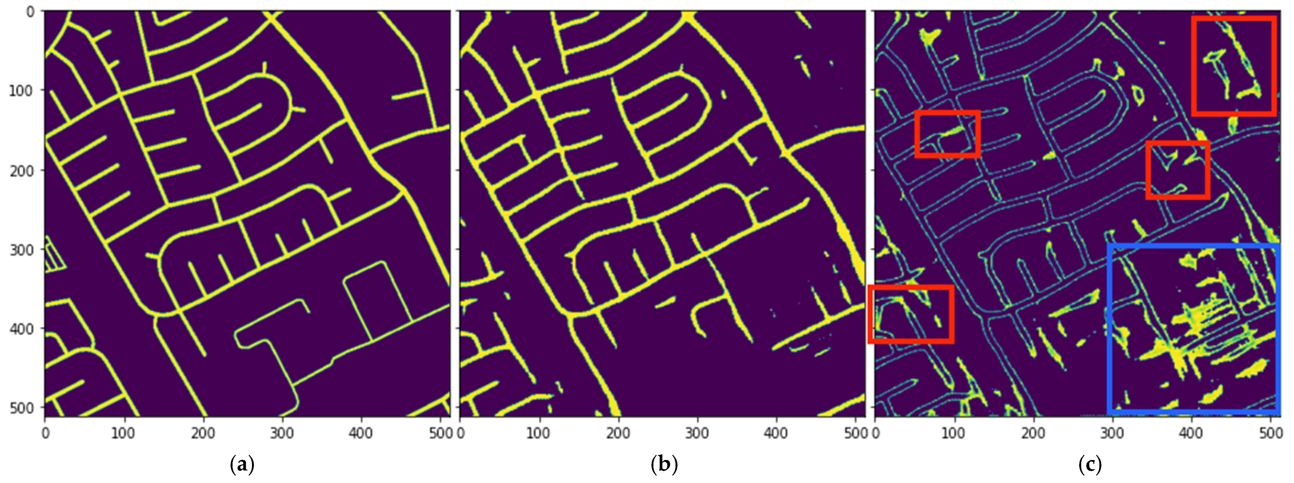
To provide a way forward, we observe that we can improve our uncertainty measurement by simply decreasing the selection threshold (increasing the recall) of road predictions. Specifically, for our model’s two class per pixel output, instead of selecting the class with the highest softmax confidence, i.e., the max[class1, class2] over each pixel, we say that the pixel is a road if the softmax score for the road class exceeds a threshold. We then measure the effectiveness of uncertainty measurements over road pixels when using varying thresholds in the range [0.01,0.5] (0 indicates the model is 100% confident the pixel is not a road, 0.5 indicates the model is undecided and 1.0 indicates 100% confident the pixel is a road). We thus include non-road predictions (at varying thresholds of confidence) in our uncertainty measurement.
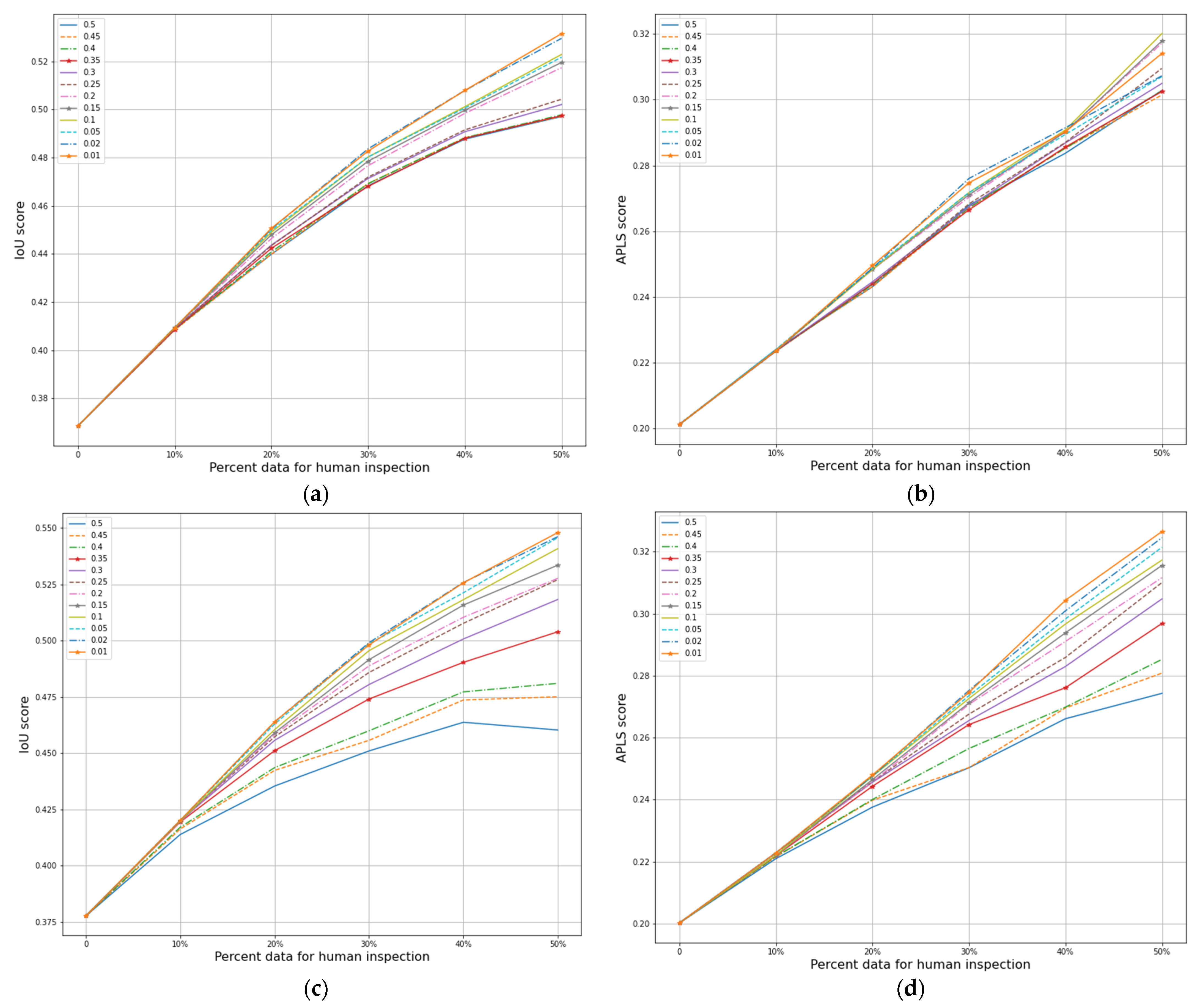
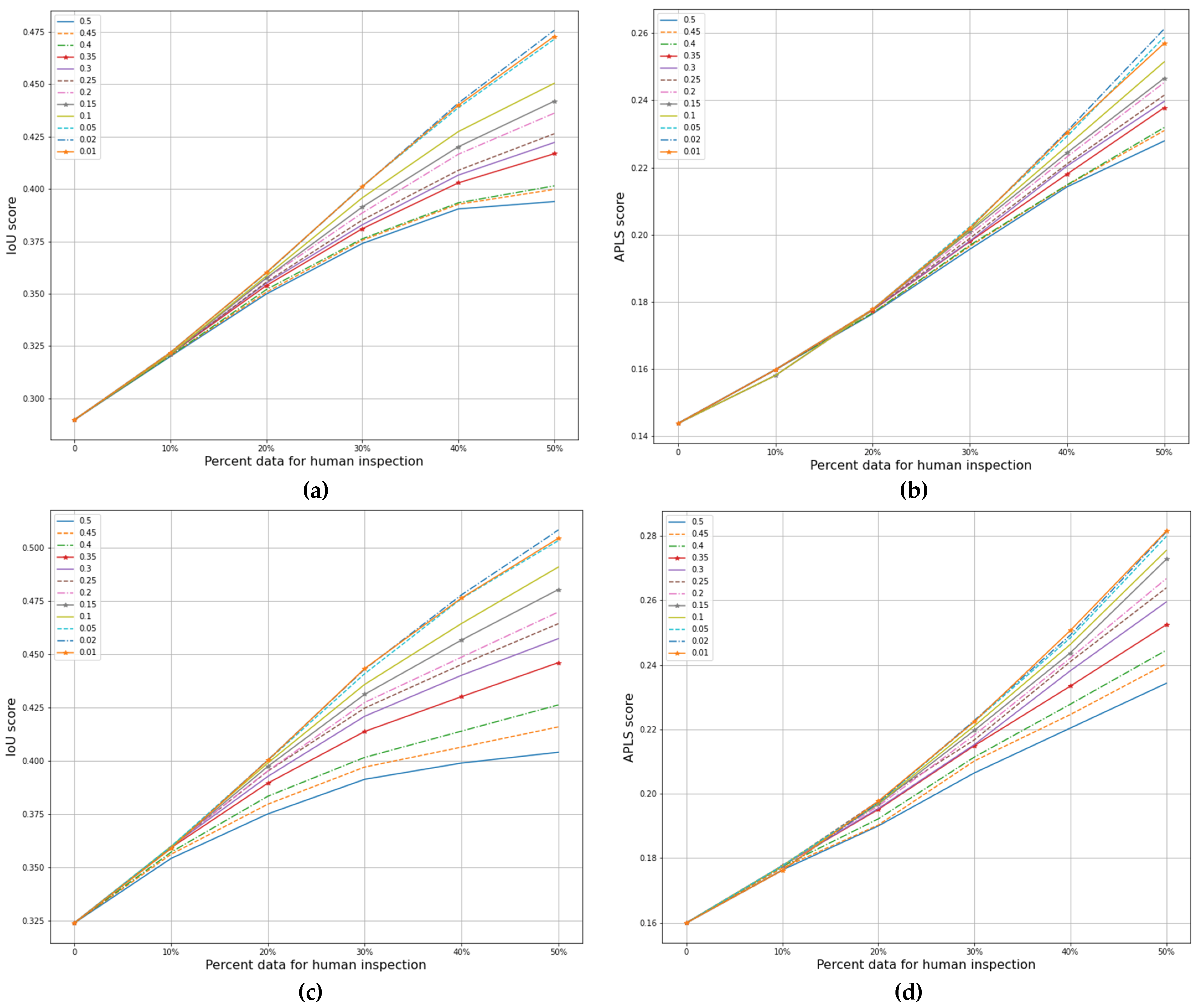
This increases the number of road pixels in the set of pixels used to measure uncertainty by drawing them from connective regions and road boundaries (Figure 6). Note that we do not modify model predictions used for scoring IoU and APLS; we only change the prediction threshold of road pixels to take our uncertainty measurement. Therefore, increasing recall for uncertainty measurement does not change the false positive or false negative rate in per-image chip scoring. It does, however, change the overall false positive/false negative rate across the test set. This is desirable, evidenced by the fact that IoU and APLS scores increase substantially when thresholding image chips according to this method of uncertainty measurement (Figures 7, 8, and 10).

2.6. Training and Testing

All models were implemented and trained using PyTorch 1.3 on four NVIDIA Tesla V100 GPUs. Training progressed using the ADAM optimizer with a learning rate of 1 × 10⁻³. MCD models were trained multiple times to perform a parameter search over optimal dropout rates, with 0.09 found to be best. L2 regularization was set to 1 × 10⁻⁵ for MCD models; no L2 regularization was used on deterministic models. Batch sizes of 16 were found to be best for the deterministic models, while a batch size of 48 performed best for MCD models. No pretraining (e.g., from ImageNet) was used, as this was found to produce lower scores. The loss function was an unweighted sum of IoU and cross-entropy (Section 2.4). Deterministic models were selected from training runs of up to 200 epochs, and MCD models were selected from training runs up to 300 epochs.
During testing, each image chip was run through the model 25 times (see Equation (6)) for MCD, and five models were used to generate the DE average. Increasing the sampling rate for MCD did not provide improvement.

3. Results

3.1. In-Distribution Test Data

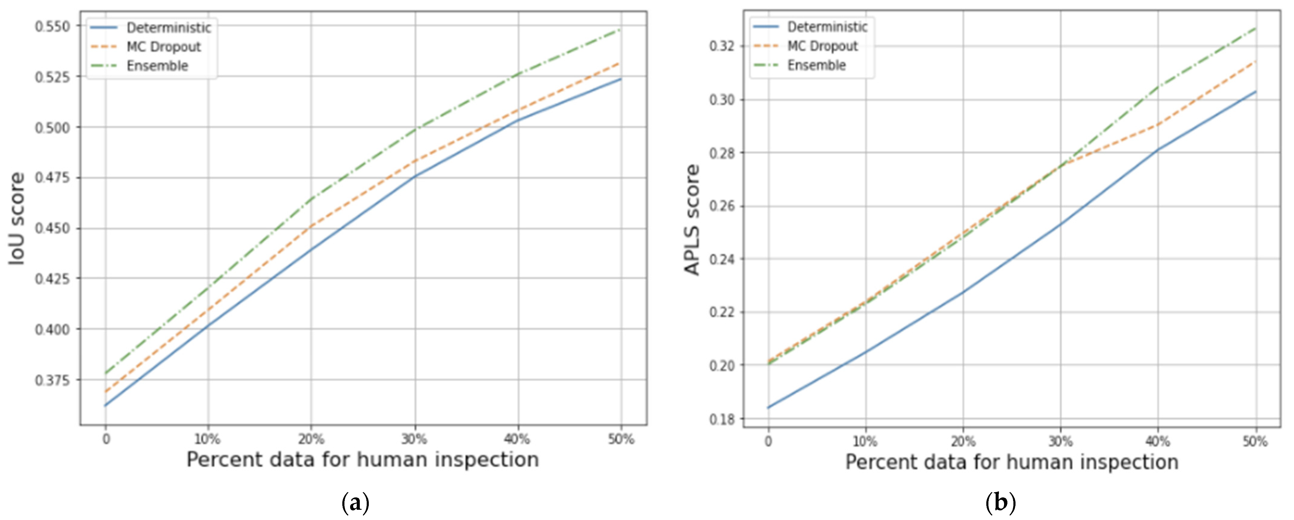
Table 1 shows results of the best models, selected from multiple training runs, over the test set before assessing performance in quality thresholding. As noted earlier, a direct comparison to other SAR road extraction models is not possible due to the lack of a standard image dataset. As expected, DEs perform best, followed by MCD. Interestingly, MCD matches the performance of DEs in the APLS score. These initial results suggest that the small gain provided by DEs may not be worth the additional computational complexity. However, our uncertainty quality results increase this performance gap and indicate, as we expected, that a simple performance baseline such as Table 1 is not sufficient to make a decision about model architecture for this task. Further results support DEs as the best method for both uncertainty estimation and performance.
Our proposed method of increasing the recall of road pixels used for uncertainty measurement (Section 2.5) improves IoU and APLS scores substantially. This effect was most pronounced in DEs, where we observed a nearly 3% IoU increase when allowing 20% of data to be submitted to human reviewers, and a nearly 9% IoU increase when submitting 50% of data (Figure 7c,d). Similar, but slightly smaller, improvements were noted when we applied this process to MCD and the deterministic model (Figure 7a,b). Across all model types, the effect size grows monotonically as the number of thresholded images increases. Since increasing recall for both pixels used for uncertainty measurement and pixels used for image scoring did not improve scores as much as doing only the former, we note that this is not a simple issue of calibration. In other words, the model is not simply assigning too low a probability to false negatives (Figure 6). Rather, increasing recall only on road pixels used for uncertainty measurement and not on predictions used for scoring supports our hypothesis: connective regions of road networks provide essential uncertainty information beyond that measurable in road predictions alone.
It is difficult to ascertain why this effect is more pronounced for ensembles. One hypothesis is that when ensembles do predict a road, they tend more often to be correct than MCD, and tend also to express less uncertainty about the choice. This results in more image predictions that are “confident” but contain significant segmentation errors. The inclusion of less confident regions via an increase in recall then exposes key areas of uncertainty that correlate more strongly with segmentation quality.
Model performance, using a BMA (or softmax point estimate, in the case of the deterministic model) at various rates of data retention is shown in Figure 8. As expected, DEs perform best, followed by MCD, although MCD performs comparatively well on the APLS score. Table 2 indicates that DEs not only produce better segmentation across images of varying uncertainty (AUC metric), but also improve more as increasingly confident images are thresholded (SUG metric). In other words, as more images are thresholded for human inspection, DEs are better able to select those with more segmentation problems than MCD and deterministic models can. This supports a growing body of evidence that ensembles are currently the best way to deal with uncertainty in DL.
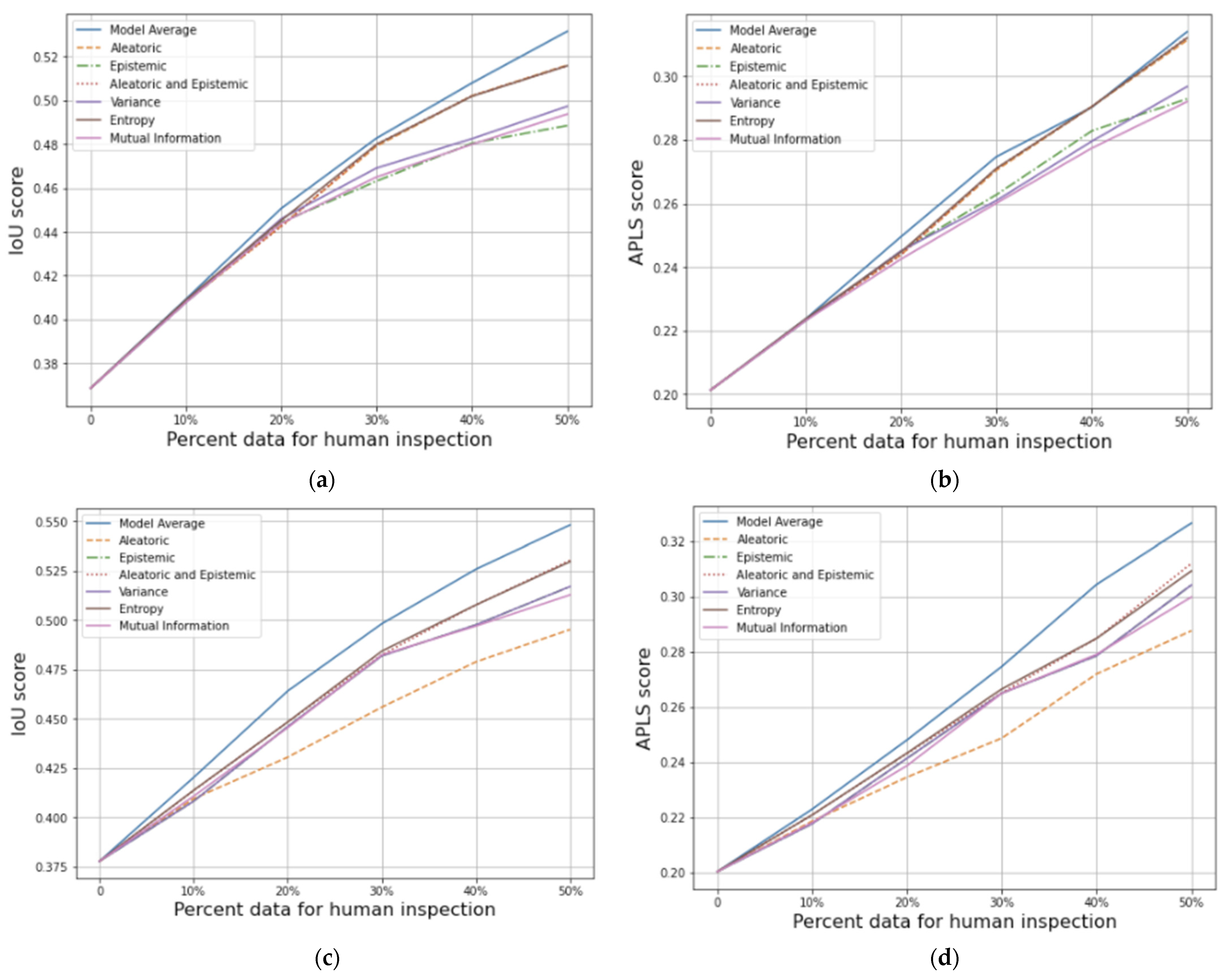
All other measures of uncertainty (variance, mutual information, etc.) provide no improvement for quality thresholding (Figure 9) over BMAs. Performance is worse in both MCD and DE models. This indicates that these methods are able to come up with a reasonable posterior mode estimate, but do not adequately model the posterior distribution. This is not entirely surprising: as noted above, MCD can only perform an approximation of the posterior distribution, and the choice of prior may not be ideal. For DEs, only five models are used, and this few samples may be too small to derive an accurate posterior. Both issues remain an open problem in deep learning and should be explored in future research.

3.2. Out-of-Distribution Test Data

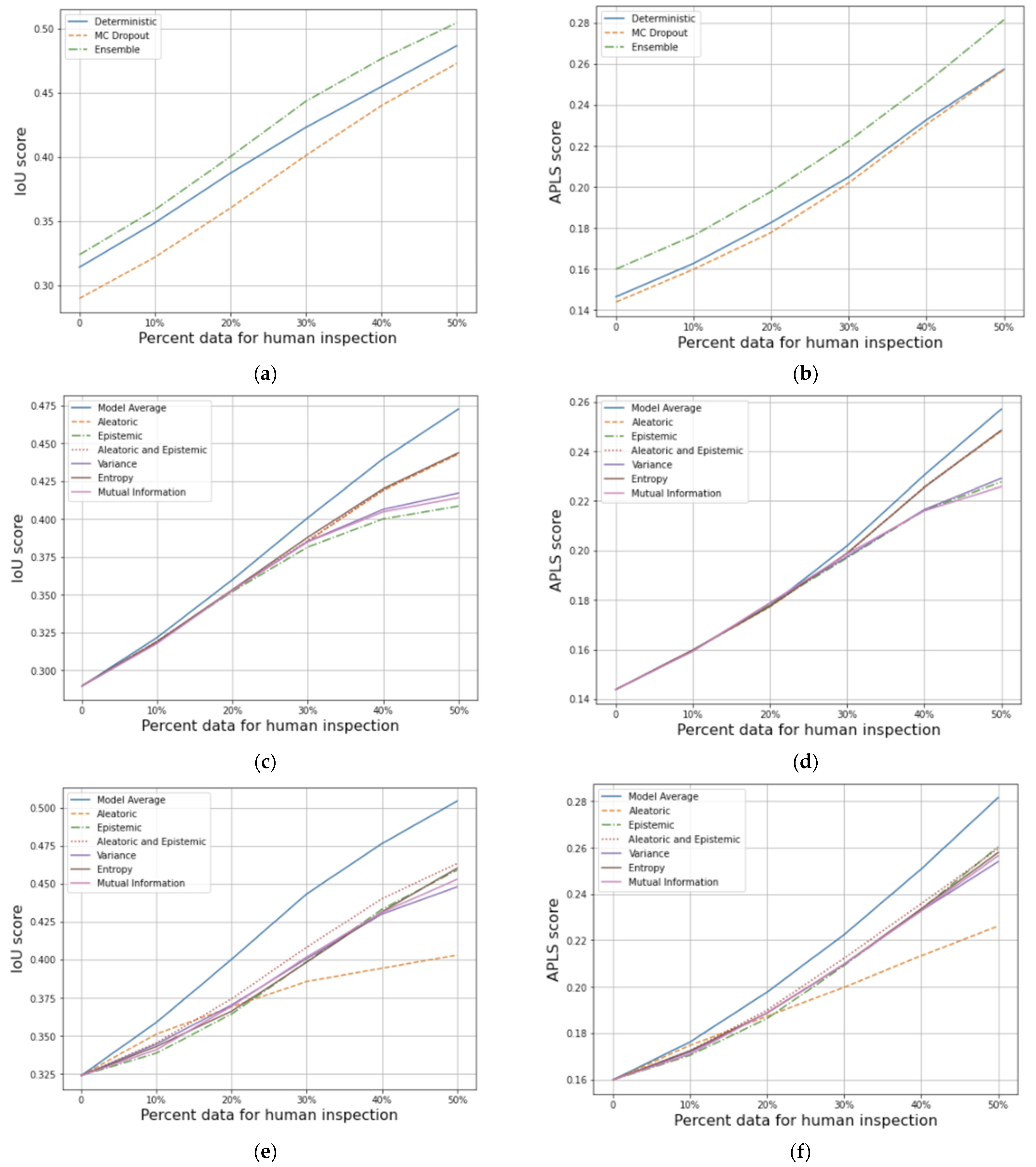
Once again, our proposed method of increasing the recall of road pixels used for uncertainty measurement, as described in Section 2.5, improves IoU and APLS scores substantially during thresholding (Figure 10). DEs again performed best across all metrics for the OOD test set. In contrast to ID data, deterministic models performed better than MCD models (Figure 11a,b). Model averages again proved more useful than all other measurements (Table 3, Figure 11c–f).
Notably, the MCD model thresholds out more OOD data than the DE, but DEs are much better at identifying the most poorly segmented data (Table 4). This is because OOD image chips are still SAR chips, albeit with corruption (Figure 1b), and the DE is better at segmenting both ID and OOD chips. Interestingly, deterministic models outperformed MCD despite the fact that MCD was better able to identify OOD examples. We discuss why this might be the case in Section 4.

4. Discussion

This paper explored a method to measure uncertainty to optimize human intervention levels in automated road segmentation pipelines that use DL. While others’ previous research has indicated that MCD and DEs can provide an uncertainty measurement more useful than the softmax output of a single deterministic model, that research focused primarily on medical imaging and autonomous driving domains. There is not, as of yet, research assessing the comparative usefulness of the most popular uncertainty methods with respect to the unique challenges of SAR segmentation tasks.
Our results presented in the previous section suggest that MCD models score higher than deterministic models for the ID test set, although this seems to be primarily due to improved model performance (as indicated by AUC scores) and not so much uncertainty information revealing segmentation quality (as indicated by SUG scores). This performance improvement is possibly due to the regularizing effect of dropout [42]. This regularization could also explain the counter-intuitive result that MCD performed more poorly than its deterministic counterpart on the OOD test data. DL models are highly underspecified and can learn numerous “predictors” that score well on a test set but are only indirectly related to the task in question [48]. It is possible that the deterministic model was able to learn such a correlation that coincidently enhanced its segmentation capability with the speckled (OOD) data, while MCD models were more restricted to learning predictors more relevant to ID data, due to the regularization induced by dropout. This would also explain the higher percentage of OOD images that MCD included in the image chip set thresholded for human intervention. In other words, MCD was indeed more aware of “what it didn’t know,” but the deterministic model was simply able to segment both ID and OOD images better.
Surprisingly, uncertainty measurements across the predictive distribution (i.e., mutual information, variance etc.) did not surpass BMAs on any score or amount of thresholding. This suggests that posterior approximations may be inadequate. Additionally, we had hypothesized that the epistemic-aleatoric distinction might correlate with different segmentation quality issues. For example, most label noise (which should correlate with higher aleatoric uncertainty) should arise from variations in the widths of roads. We speculated that this edge noise would impact IoU more than APLS, since variations at road edges do not result in connectivity changes. However, this does not seem to be the case, as there is no distinct correlation between aleatoric or epistemic uncertainty and segmentation metrics that would allow for the optimization of human intervention according to one metric rather than the other. This is at least partly due to the fact that aleatoric and epistemic uncertainty overlap significantly across pixels (at least in the manner defined by Kwon et al. [14]). Additionally, wider road structures with gaps in mid regions can also create topology differences when converted to graphs, e.g., such roads may be converted to two roads instead of one. We may have underestimated these kinds of effects and the noise they contribute to an epistemic-aleatoric distinction. Assessing this fully is beyond the scope of this paper, but an interesting subject for future research.
In both ID and OOD cases, epistemic uncertainty correlated more strongly with segmentation quality in DEs than aleatoric uncertainty. This was not observed in the MCD model. This may be further evidence that DEs provide much greater model diversity than MCD [44]. Possibly, since models in the DE are trained separately, they can optimize over different problem spaces. In MCD, the model must optimize over a single problem space, given the single local minimum it converges to. This would allow different models in the DE to express very diverse softmax scores about an uncertain pixel (epistemic uncertainty), while contrarily the MCD would generate multiple similar softmax scores (aleatoric uncertainty).
Furthermore, the results of ID and OOD experiments indicate that our method of measuring uncertainty over predicted road pixels with a low decision threshold increases the usefulness of the examined DL methods. This is evidenced by relatively stable SUG scores (which disentangle uncertainty usefulness from model performance) across ID and OOD data. As discussed in Section 1.1 and Section 2.1, though we would expect the segmentation performance of models to fluctuate substantially across models trained or tested on varying SNR images, our results suggest that our proposed uncertainty measurement will yield reasonably consistent and useful results.

5. Conclusions

This paper developed a quantitative method to measure uncertainty to optimize human intervention levels in automated road segmentation pipelines that use DL on SAR images. We showed that uncertainty must be measured over a set of predicted road pixels in order to be effective, and that, most importantly, the uncertainty information provided by this set can be significantly improved by including road pixels with lower softmax scores.
Deep ensembles (DE) outperform Monte Carlo dropout (MCD) and deterministic models on both in-distribution and out-of-distribution data. With DEs, we were able to achieve an IoU increase of almost 3% when sending 20% of test data for quality inspection, and nearly 9% when sending 50% of data for quality inspection. We provide more evidence that DEs have advantages over single models, although this comes at increased computational cost. Despite this cost, DEs are likely the best option for most real-world applications due to their superior performance, as noted in Table 2 and Table 3.
In future research, we would like to explore the development of alternative methods that can achieve state-of-the-art performance and uncertainty without invoking ensembles. We would also like to explore how different uncertainty measurements correlate with specific segmentation errors. For example, it would be useful to tailor the system to threshold less morphological or topological error, as the situation warranted. Finally, as discussed in Section 2.1, due to the formidable time and cost requirements of constructing a global scale road dataset, our study’s results are limited to a single SAR sensor, single incidence angle, and a relatively small geographic area. We leave the construction of such a dataset, which could improve understanding of any variability in uncertainty methods by specific types of changes in data, to future work. While much work lies ahead, we believe we have provided solid initial evidence, across ID and OOD data, that the presented techniques can be useful in a real-world, large-scale road extraction system.

Author Contributions

Conceptualization, J.H.; data curation, J.H.; investigation, J.H.; methodology, J.H.; supervision, B.R.; writing—original draft, J.H.; writing—review and editing, B.R. All authors have read and agreed to the published version of the manuscript.

Funding

This study was fully funded through the NSERC Industrial Research Chair in SAR Technology, Methods and Applications at Simon Fraser University.

Data Availability Statement

The RADARSAT-2 data used in this study is not available for public release due to licensing requirements by MDA.

Acknowledgments

We would like to William Yolland for providing a sounding-board for ideas and assisting with proof-reading the manuscript.

Conflicts of Interest

The authors declare no conflict of interest.

References

  1. Guo, C.; Pleiss, G.; Sun, Y.; Weinberger, K.Q. On Calibration of Modern Neural Networks. arXiv 2017, arXiv:170604599. [Google Scholar]
  2. Gal, Y.; Ghahramani, Z. Dropout as a Bayesian Approximation: Representing Model Uncertainty in Deep Learning. arXiv 2016, arXiv:150602142. [Google Scholar]
  3. Henne, M.; Schwaiger, A.; Roscher, K.; Weiss, G. Benchmarking Uncertainty Estimation Methods for Deep Learning with Safety-Related Metrics. In Proceedings of the 34th AAAI Conference on Artificial Intelligence SafeAI, New York, NY, USA, 9–12 February 2020; p. 8. [Google Scholar]
  4. Loquercio, A.; Segù, M.; Scaramuzza, D. A General Framework for Uncertainty Estimation in Deep Learning. IEEE Robot. Autom. Lett. 2020, 5, 3153–3160. [Google Scholar] [CrossRef] [Green Version]
  5. Leibig, C.; Allken, V.; Ayhan, M.S.; Berens, P.; Wahl, S. Leveraging Uncertainty Information from Deep Neural Networks for Disease Detection. Sci. Rep. 2017, 7, 17816. [Google Scholar] [CrossRef] [PubMed] [Green Version]
  6. Kendall, A.; Gal, Y. What Uncertainties Do We Need in Bayesian Deep Learning for Computer Vision? arXiv 2017, arXiv:170304977. [Google Scholar]
  7. Ovadia, Y.; Fertig, E.; Ren, J.; Nado, Z.; Sculley, D.; Nowozin, S.; Dillon, J.V.; Lakshminarayanan, B.; Snoek, J. Can You Trust Your Model’s Uncertainty? Evaluating Predictive Uncertainty Under Dataset Shift. arXiv 2019, arXiv:190602530. [Google Scholar]
  8. Nixon, J.; Dusenberry, M.; Jerfel, G.; Nguyen, T.; Liu, J.; Zhang, L.; Tran, D. Measuring Calibration in Deep Learning. arXiv 2020, arXiv:190401685. [Google Scholar]
  9. Nalisnick, E.; Matsukawa, A.; Teh, Y.W.; Gorur, D.; Lakshminarayanan, B. Do Deep Generative Models Know What They Don’t Know? arXiv 2019, arXiv:181009136. [Google Scholar]
  10. Wilson, A.G.; Izmailov, P. Bayesian Deep Learning and a Probabilistic Perspective of Generalization. arXiv 2020, arXiv:200208791. [Google Scholar]
  11. Maddox, W.; Garipov, T.; Izmailov, P.; Vetrov, D.; Wilson, A.G. A Simple Baseline for Bayesian Uncertainty in Deep Learning. arXiv 2019, arXiv:190202476. [Google Scholar]
  12. Lakshminarayanan, B.; Pritzel, A.; Blundell, C. Simple and Scalable Predictive Uncertainty Estimation Using Deep Ensembles. arXiv 2017, arXiv:161201474. [Google Scholar]
  13. Chen, L.-C.; Zhu, Y.; Papandreou, G.; Schroff, F.; Adam, H. Encoder-Decoder with Atrous Separable Convolution for Semantic Image Segmentation. arXiv 2018, arXiv:180202611. [Google Scholar]
  14. Kwon, Y.; Won, J.-H.; Kim, B.; Paik, M. Uncertainty Quantification Using Bayesian Neural Networks in Classification: Application to Biomedical Image Segmentation. Comput. Stat. Data Anal. 2020, 142, 106816. [Google Scholar] [CrossRef]
  15. Steger, C.; Glock, C.; Eckstein, W.; Mayer, H.; Radig, B. Model-Based Road Extraction from Images. In Automatic Extraction of Man-Made Objects from Aerial and Space Images; Gruen, A., Kuebler, O., Agouris, P., Eds.; Birkhäuser: Basel, Switzerland, 1995; pp. 275–284. [Google Scholar]
  16. Hedman, K.; Wessel, B.; Soergel, U.; Stilla, U. Automatic road extraction by fusion of multiple SAR views. In Proceedings of the 3th International Symposium: Remote Sensing and Data Fusion on Urban Areas, Tempe, AZ, USA, 14–16 March 2005. [Google Scholar]
  17. Hinz, S.; Baumgartner, A.; Steger, C.; Mayer, H.; Eckstein, W.; Ebner, H.; Radig, B.; Smati, S.M. Road Extraction in Rural and Urban Areas. In Semantic Modeling for the Acquisition of Topographic Information from Images and Maps; Birkhäuser: Basel, Switzerland, 1999. [Google Scholar]
  18. Steger, C.; Mayer, H.; Radig, B. The Role of Grouping for Road Extraction. In Automatic Extraction of Man-Made Objects from Aerial and Space Images (II); Birkhäuser: Basel, Switzerland, 1997. [Google Scholar]
  19. Xu, R.; He, C.; Liu, X.; Chen, D.; Qin, Q. Bayesian Fusion of Multi-Scale Detectors for Road Extraction from SAR Images. ISPRS Int. J. Geo. Inf. 2017, 6, 26. [Google Scholar] [CrossRef] [Green Version]
  20. Elguebaly, T.; Bouguila, N. A Bayesian Approach for SAR Images Segmentation and Changes Detection. In Proceedings of the 25th Biennial Symposium on Communications, Kingston, ON, Canada, 12–14 May 2010; pp. 24–27. [Google Scholar]
  21. Zhao, Q.; Li, Y.; Liu, Z. SAR Image Segmentation Using Voronoi Tessellation and Bayesian Inference Applied to Dark Spot Feature Extraction. Sensors 2013, 13, 14484–14499. [Google Scholar] [CrossRef] [Green Version]
  22. Melgani, F.; Bruzzone, L. Classification of Hyperspectral Remote Sensing Images with Support Vector Machines. IEEE Trans. Geosci. Remote Sens. 2004, 42, 1778–1790. [Google Scholar] [CrossRef] [Green Version]
  23. Yager, N.; Sowmya, A. Support Vector Machines for Road Extraction from Remotely Sensed Images. In Computer Analysis of Images and Patterns, Proceedings of the CAIP 2003, Groningen, The Netherlands, 25–27 August 2003; Springer: Berlin/Heidelberg, Germany; Volume 2756.
  24. Yousif, O.; Ban, Y. Improving SAR-Based Urban Change Detection by Combining MAP-MRF Classifier and Nonlocal Means Similarity Weights. IEEE J. Sel. Top. Appl. Earth Obs. Remote Sens. 2014, 7, 4288–4300. [Google Scholar] [CrossRef]
  25. Zeiler, M.D.; Fergus, R. Visualizing and Understanding Convolutional Networks. arXiv 2014, arXiv:abs/1311.2901. [Google Scholar]
  26. Krizhevsky, A.; Sutskever, I.; Hinton, G.E. ImageNet Classification with Deep Convolutional Neural Networks. Commun. ACM 2012, 60, 84–90. [Google Scholar] [CrossRef]
  27. Kemker, R.; Salvaggio, C.; Kanan, C. Algorithms for Semantic Segmentation of Multispectral Remote Sensing Imagery Using Deep Learning. ISPRS J. Photogramm. Remote Sens. 2018, 145, 60–77. [Google Scholar] [CrossRef] [Green Version]
  28. Seo, H.; Khuzani, M.B.; Vasudevan, V.; Huang, C.; Ren, H.; Xiao, R.; Jia, X.; Xing, L. Machine Learning Techniques for Biomedical Image Segmentation: An Overview of Technical Aspects and Introduction to State-of-Art Applications. Med. Phys. 2020, 47, e148–e167. [Google Scholar] [CrossRef]
  29. Zhang, Q.; Kong, Q.; Zhang, C.; You, S.; Wei, H.; Sun, R.; Li, L. A New Road Extraction Method Using Sentinel-1 SAR Images Based on the Deep Fully Convolutional Neural Network. Eur. J. Remote Sens. 2019, 52, 572–582. [Google Scholar] [CrossRef] [Green Version]
  30. Henry, C.; Azimi, S.M.; Merkle, N. Road Segmentation in SAR Satellite Images with Deep Fully Convolutional Neural Networks. IEEE Geosci. Remote Sens. Lett. 2018, 15, 1867–1871. [Google Scholar] [CrossRef] [Green Version]
  31. Xiong, D.; He, C.; Liu, X.; Liao, M. An End-To-End Bayesian Segmentation Network Based on a Generative Adversarial Network for Remote Sensing Images. Remote Sens. 2020, 12, 216. [Google Scholar] [CrossRef] [Green Version]
  32. Wen, Y.; Vicol, P.; Ba, J.; Tran, D.; Grosse, R.B. Flipout: Efficient Pseudo-Independent Weight Perturbations on Mini-Batches. arXiv 2018, arXiv:abs/1803.04386. [Google Scholar]
  33. Hernández-Lobato, J.M.; Adams, R. Probabilistic Backpropagation for Scalable Learning of Bayesian Neural Networks. In Proceedings of the 32nd International Conference on Machine Learning, Lille, France, 6–11 July 2015. [Google Scholar]
  34. Nair, T.; Precup, D.; Arnold, D.; Arbel, T. Exploring Uncertainty Measures in Deep Networks for Multiple Sclerosis Lesion Detection and Segmentation. arXiv 2018, arXiv:abs/1808.01200. [Google Scholar]
  35. McClure, P.; Rho, N.; Lee, J.A.; Kaczmarzyk, J.R.; Zheng, C.Y.; Ghosh, S.; Nielson, D.M.; Thomas, A.G.; Bandettini, P.; Pereira, F. Knowing What You Know in Brain Segmentation Using Bayesian Deep Neural Networks. Front. Neuroinformatics 2019, 13, 67. [Google Scholar] [CrossRef] [PubMed]
  36. Filos, A.; Farquhar, S.; Gomez, A.N.; Rudner, T.G.J.; Kenton, Z.; Smith, L.; Alizadeh, M.; Kroon, A.D.; Gal, Y. A Systematic Comparison of Bayesian Deep Learning Robustness in Diabetic Retinopathy Tasks. arXiv 2019, arXiv:abs/1912.10481. [Google Scholar]
  37. Hendrycks, D.; Dietterich, T.G. Benchmarking Neural Network Robustness to Common Corruptions and Perturbations. arXiv 2019, arXiv:abs/1903.12261. [Google Scholar]
  38. Pu, W. Deep SAR Imaging and Motion Compensation. IEEE Trans. Image Process. 2021, 30, 2232–2247. [Google Scholar] [CrossRef] [PubMed]
  39. Ronneberger, O.; Fischer, P.; Brox, T. U-Net: Convolutional Networks for Biomedical Image Segmentation. arXiv 2015, arXiv:abs/1505.04597. [Google Scholar]
  40. Saxe, A.M.; Bansal, Y.; Dapello, J.; Advani, M.; Kolchinsky, A.; Tracey, B.D.; Cox, D. On the Information Bottleneck Theory of Deep Learning. In Proceedings of the 6th International Conference on Learning Representations, Vancouver, BC, Canada, 30 April–3 May 2018. [Google Scholar]
  41. Bishop, C.M. Pattern Recognition and Machine Learning (Information Science and Statistics); Springer: New York, NY, USA, 2006. [Google Scholar]
  42. Hinton, G.E.; Srivastava, N.; Krizhevsky, A.; Sutskever, I.; Salakhutdinov, R. Improving Neural Networks by Preventing Co-Adaptation of Feature Detectors. arXiv 2012, arXiv:abs/1207.0580. [Google Scholar]
  43. Shannon, C. A Mathematical Theory of Communication. Bell. Syst. Tech. J. 1948, 27, 379–423. [Google Scholar] [CrossRef] [Green Version]
  44. Fort, S.; Hu, H.; Lakshminarayanan, B. Deep Ensembles: A Loss Landscape Perspective. arXiv 2019, arXiv:abs/1912.02757. [Google Scholar]
  45. Jaccard, P. The Distribution of the Flora in the Alpine Zone. New Phytol. 1912, 11, 37–50. [Google Scholar] [CrossRef]
  46. Rahman, M.A.; Wang, Y. Optimizing Intersection-Over-Union in Deep Neural Networks for Image Segmentation. In Proceedings of the 12th International Symposium ISVC, Las Vegas, NV, USA, 12–14 December 2016. [Google Scholar]
  47. Etten, A.V.; Lindenbaum, D.; Bacastow, T.M. SpaceNet: A Remote Sensing Dataset and Challenge Series. arXiv 2018, arXiv:abs/1807.01232. [Google Scholar]
  48. D’Amour, A.; Heller, K.; Moldovan, D.; Adlam, B.; Alipanahi, B.; Beutel, A.; Chen, C.; Deaton, J.; Eisenstein, J.; Hoffman, M.D.; et al. Underspecification Presents Challenges for Credibility in Modern Machine Learning. arXiv 2020, arXiv:2011.03395. [Google Scholar]
Figure 1. (a) The complete SAR image prior to chipping into 512 × 512 px regions for model ingestion. (b) Image chip after multi-temporal filtering, from the ID dataset. (c) The same image chip with speckle from the out-of-distribution (OOD) dataset. The speckled images have much noisier texture, which results in a different data distribution and poorer segmentation quality than filtered counterparts (note that a model trained on speckled images would have poorer performance with filtered images).
Remotesensing 13 01472 g001
Figure 2. Our modified DeepLab model. Since roads can have thickness less than the output stride (the number of input pixels represented by one output pixel) of the standard ResNet backbone, we reduce output stride by reducing downsampling in the backbone. We downsample only twice, such that the output stride of the network becomes four. This allows the fine-grain segmentation that we need to extract thin objects such as roads, while the ASPP layer still allows for high-context information to inform local decisions.
Remotesensing 13 01472 g002
Figure 3. (a) The Intersection over Union score is not well calibrated, i.e., image chips with low scores have confident softmax values, despite producing a well-trained model. This is problematic, as it prevents thresholding of low scoring image chips based on network output. (b) A loss function composed of the sum of IoU and cross-entropy losses provides a well calibrated threshold ramp, while maintaining model performance.
Remotesensing 13 01472 g003aRemotesensing 13 01472 g003b
Figure 4. (a) The average path length score (APLS) code takes a ground truth label and prediction from the segmentation network and converts those images to graph representations [47]. In this example, the proposal graph resulting from the predicted image is missing connective edges (roads). This results in a longer optimal path between the two points illustrated in the lower two images, and a lower APLS score. (b) Ground truth image chip. (c) APLS is heavily penalized (0.06) due to missing connective regions, and the addition of a false positive section in the upper middle of the image chip. Intersection over union (IoU) scores relatively high (0.66), despite this.
Remotesensing 13 01472 g004
Figure 5. IoU (a) and APLS (b) do not correlate with entropy per image chip, despite the fact that entropy is well correlated with average pixel-wise segmentation accuracy per chip (c). IoU and APLS are much better measures of the segmentation performance of the model.
Remotesensing 13 01472 g005
Figure 6. Ground truth (a), softmax predictions (b) (higher is brighter) and softmax predictions (c) in [0.01,0.5] (lower is brighter). Non-road predictions tend to be very confident (i.e., near zero; dark regions). Uncertainty tends to increase in connective regions (as denoted by red and blue squares). However, as the region inside the blue square indicates, this is not simply a matter of calibration. Selecting these pixels for uncertainty measurement would appropriately increase uncertainty; however, lowering the threshold for road prediction measurement in this region would result in a very high false positive rate.
Remotesensing 13 01472 g006
Figure 7. Performance comparison of MCD (a,b) and DE (c,d) model averages over varying decision thresholds for ID data. Scores increase substantially when using lower road class thresholds for uncertainty measurements, which are displayed for thresholds in the range [0.01,0.5] for the ID test set. This effect increases as more (higher confidence) image chips are sent to humans for quality assurance. The effect is more than twice as large for the DE than for MCD. The effect size for the deterministic model (not pictured) is similar to MCD.
Remotesensing 13 01472 g007
Figure 8. IoU (a) and APLS scores (b) over data retention rates for ID data. DEs provide the best performance overall, and MCD outperformed the deterministic model.
Remotesensing 13 01472 g008
Figure 9. Performance comparison of aleatoric, epistemic, variance, entropy and mutual information uncertainty measurements against model averages for MCD (a,b) and DE (c,d) with ID data. Model averages perform better at all levels of thresholding. In the MCD case, the magnitude of epistemic uncertainty is small enough that it adds almost nothing to the aleatoric measurement when combined. Interestingly, epistemic measurements are more useful than aleatoric in the DE model, and vice-versa for the MCD model. This evidences the idea that DEs provide more diverse support to the predictive distribution than samples from MCD models.
Remotesensing 13 01472 g009
Figure 10. Performance comparison of MCD (a,b) and DE (c,d) model averages over varying decision thresholds for OOD data. Scores again increase substantially with the OOD test set when using lower road class thresholds, which are displayed for thresholds in the range [0.01,0.5]. This effect increases as more (higher confidence) image chips are sent to humans for quality assurance. The effect is more than twice as large for the DE than for MCD. The effect size for the deterministic model (not pictured) is similar to MCD. The stability of these results across ID and OOD data supports the generalizability of our method.
Remotesensing 13 01472 g010
Figure 11. IoU (a) and APLS scores (b) over data retention rates for OOD data, and performance comparison of aleatoric, epistemic, variance, entropy and mutual information measurements with MCD (c,d) and DE (e,f) model averages on OOD data. As with ID data, DE’s perform best, and model averages perform better than other measurements at all levels of data retention.
Remotesensing 13 01472 g011
Table 1. Best model results on test data, selected from multiple training runs. Each score is the average over all image chips in the test set. MCD matches DEs on APLS, but DEs perform best overall.
MethodIoUAPLS
Deterministic0.3620.184
MC Dropout0.3690.201
Deep Ensemble0.3780.200
Table 2. Summary of model performance over all levels of data retention for ID data. Calculated from results plotted in Figure 8.
MethodSUG IoUSUG APLSTotal SUGAuC IoUAuC APLSTotal AuC
Deterministic0.5320.3490.8812.261.213.47
MC Dropout0.5400.3460.8852.301.303.60
Deep Ensemble0.5670.3750.9422.371.313.69
Table 3. Summary of results of model performance in OOD data at varying amounts of thresholding for quality assessment.
MethodSUG IoUSUG APLSTotal SUGAuC IoU 2AuC APLSTotal AuC
Deterministic0.5300.3080.8382.010.9843.00
MC Dropout0.5470.3080.8551.900.9692.87
Deep Ensemble0.5640.3290.8932.091.073.16
Table 4. Percentage of OOD image chips that get thresholded for quality assessment, out of the total number of image chips that gets thresholded at each data retention tier, i.e. if number is higher, the method includes more OOD image chips in the total batch sent for human review.
Method10%20%30%40%50%
Deterministic0.90.70.630.60.58
MC Dropout0.90.80.730.70.66
Deep Ensemble0.70.650.630.650.62
Publisher’s Note: MDPI stays neutral with regard to jurisdictional claims in published maps and institutional affiliations.