Abstract
While terrestrial laser scanning and photogrammetry provide high quality point cloud data that can be used for rock slope monitoring, their increased use has overwhelmed current data analysis methodologies. Accordingly, point cloud processing workflows have previously been developed to automate many processes, including point cloud alignment, generation of change maps and clustering. However, for more specialized rock slope analyses (e.g., generating a rockfall database), the creation of more specialized processing routines and algorithms is necessary. More specialized algorithms include the reconstruction of rockfall volumes from clusters and points and automatic classification of those volumes are both processing steps required to automate the generation of a rockfall database. We propose a workflow that can automate all steps of the point cloud processing workflow. In this study, we detail adaptions to commonly used algorithms for rockfall monitoring use cases, such as Multiscale Model to Model Cloud Comparison (M3C2). This workflow details the entire processing pipeline for rockfall database generation using terrestrial laser scanning.
1. Introduction
Ease of use and reduction of cost has led to an increased application of terrestrial laser scanning (TLS) and photogrammetry in a wide range of earth science applications. A review of earth science research using photogrammetry and terrestrial laser scanning by Telling et al. [1] notes that the number of publications using and citing methods including TLS has increased at a near exponential rate since 1995. While these methods result in the same type of raw data (e.g., using a lidar scanner to acquire point clouds or using structure from motion to construct point clouds from images), the applications in earth science are incredibly diverse. Point clouds can be used to create DEMs which have been used to map snow depth and movement [2,3,4]. In geomorphology, TLS and photogrammetry have been used to better understand erosional and depositional processes [5,6,7,8]. Likewise, TLS and photogrammetry have been implemented to perform rock slope characterization and monitoring for rockfall and landslide hazards [1,9].
In the past decade, TLS has become a commonly used method for slope monitoring and rockmass characterization [1,9,10,11]. As the amount of research in this field has increased, many applications of TLS have been developed including modelling rockfall volumes and fall scarps [1,9,12,13], conducting hazard and risk surveys [1,14,15] and analyzing trends using magnitude-frequency curves [16,17,18,19,20]. Recent studies have used TLS to generate rockfall databases, which can subsequently be used for various types of analyses [18,21,22].
In regions where rockfall hazard is prevalent, high-frequency monitoring activities are beneficial to understand slope degradation over time. It has been shown that data can be collected at a near continuous rate using TLS and photogrammetry [11,23,24,25]. The rockfall data collected with these methods have many uses. A rockfall database can be used to identify precursors to larger rockfall events [18,26,27,28,29,30], examine correlations between meteorological events and rockfall [31,32,33,34], establish and modify rockfall hazard rating systems [35,36,37,38] and better understand frequency of large rockfall events [13,18,19,24,39]. A common method for examining the frequency of rockfall is the magnitude cumulative-frequency curve (MCF), which can be used to forecast the recurrence interval of large rockfalls. These curves can be described by a power-law distribution ( that is defined by rockfall volume (V) and a set of constants (a and ) (Equation (1)).
The acquisition of high frequency TLS and photogrammetry (and the resultant rockfall database) is important to the interpretation of these MCF curves. Van Veen et al. [18] showed that the amount of time between scans will directly impact the resolution of MCF curves do to spatial overlap of rockfalls. However, the large amount of data that come from high frequency monitoring means that the quantity of data acquired by TLS and photogrammetry has begun to overwhelm users [40]. As a result, workflows have been developed in order to process point cloud data in an automated or semi-automated routine [9,11,23,41,42,43]. These routines seek to align point clouds to a common coordinate system, classify and/or remove unwanted zones from the point cloud (e.g., vegetation, talus, snow), calculate the change occurring between two point clouds, extract volumes that represent rockfall and classify rockfall shapes.
However, these workflows have some notable limitations and a review of the literature has found that there are aspects of the point cloud processing workflow that have not been well-documented including parameter choices for rockfall shape reconstruction and methods for classifying point clusters to create a rockfall database, with the exception of a few more recent studies [20,44,45]. Though progress has been made to adapt and improve change detection algorithms [24,43,46], complex geometry can influence the results of these calculations. While Williams et al. [24] and Kromer et al. [23] have already developed adaptations of the commonly used Multiscale Model-to-Model Cloud Comparison (M3C2) change calculation [43], further advances are proposed in this study that have shown improvements to the performance of the change algorithm, for the purpose of identifying rockfall events. Additionally, after individual volumes are extracted from the point cloud using clustering, the process of choosing parameters for volume reconstruction (e.g., alpha radius for alpha shapes or lambda for power crust) [47,48] and filtering out erroneous volumes is typically either ignored or performed manually. This study documents these processes and proposes a way of filtering rockfalls using the random forest algorithm. All aspects of the proposed workflow were designed with the goal of creating a rockfall database that could be used for analysis of slope processes at high temporal frequency. The source code is available on GitHub (https://github.com/hschovanec-usgs/point-cloud-processing (accessed on 1 February 2021)).
2. Materials and Methods
2.1. Study Site
The study site used for testing is located approximately one mile east of Glenwood Springs, Colorado, adjacent to Interstate-70 (I70). Glenwood Canyon is active with rockslides often causing road closures multiple times per year [49]. The site near Glenwood canyon is directly adjacent to both a walking path and the highway. The Colorado Department of Transportation (CDOT) monitors rockfall in this area to determine the stability of the slope and locations along the slope where rockfall must be controlled. This slope is composed of a coarse-grained, Precambrian, megacrystic granite [50] (Figure 1).
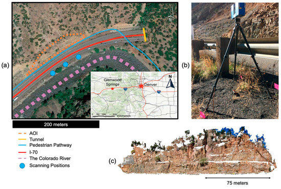
Figure 1.
(a) Location of the slope and scanning positions; (b) Example of scanning setup; (c) Point cloud representation of the slope in Glenwood Springs Colorado.
TLS data acquisition was performed using a Faro Focus 3D × 330 lidar scanner that allowed for the collection of intensity and color along with the standard x, y, z data. This scanner has two main ranging settings: “quality” and “resolution”. To provide high quality, dense point clouds for this slope at a distance of approximately 30 m from the instrument, the following settings were used: 4× quality and a ½ resolution. The 4× ensures that each data point is recorded and averaged for four times (approximately 8 µs) the baseline recording time (1 µs); ½ resolution defines a high point density for collections. The mean point density was greater than 3000 points per cubic meter and the distance between points in regions directly in front of the scanner with the highest point density was approximately 0.015 m. Three overlapping scans were collected from different viewpoints to further increase the point density and cover areas of the slope that may have been occluded from one viewpoint.
2.2. Workflow Overview
The proposed workflow follows an outline similar to those that have been previously published [18,24,41,46,51], which have four primary steps used to extract rockfall from a slope’s point cloud:
- Alignment: The process of putting one or more point cloud(s) in a common coordinate system.
- Classification: Categorizing points within the point cloud.
- Change calculation: Comparing the points between a reference cloud and a secondary (data) cloud to determine changes in point locations.
- Clustering: Labelling points by some characteristic of the points (e.g., point density).
However, a number of alterations and additions make this workflow unique. Figure 2 gives a high-level overview of the proposed workflow. The processing pipeline was written in C++ and MATLAB and implements the open-source software library, Point Cloud Library (PCL). While the parameters used in this workflow were tuned specifically for the study site, parameters can be specified using a config file and there is an option to dynamically calculate most parameters based upon point density (example configuration files can be found on GitHub at https://github.com/hschovanec-usgs/point-cloud-processing (accessed on 1 February 2021)). This makes the workflow applicable to any study site and the alignment algorithm has already been used by the authors on other slopes with minor parameter adjustments.
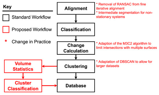
Figure 2.
Workflow overview showing the primary steps in the workflow, which is comprised of code in C++ and MATLAB. Specific inputs, outputs and steps are not shown here, but are detailed along with workflows specific to each step.
2.3. Preprocessing
For the purpose of this study, preprocessing steps were divided into two categories. The first type of preprocessing step is one required to setup the pipeline. These steps were organizational (performed at the onset to configure the pipeline) and were not automated. The second type of preprocessing step was a step that prepared the point cloud for one of the major pipeline steps (e.g., temporarily subsampling the cloud to reduce the computational time for the alignment algorithm).
The initial preprocessing steps required were as follows:
- Converting the scanner’s proprietary file format to ASCII.
- Selecting points that define the boundary of the area of interest in 3D space.
- Determining suitable ranges of parameters for the algorithms (e.g., subsampling size, normal calculation radius).
The secondary preprocessing steps included filtering, subsampling and segmenting (Table 1). The statistical outlier removal (SOR) filter was used to remove regions with highly variable point density [52]. These regions were found to be related to areas occluded from the view of the scanner and vegetated areas. Subsampling had two purposes in the proposed pipeline. First, point clouds were temporarily subsampled to expedite the alignment algorithm. The voxel grid filter in PCL is used to increase the efficiency of the course alignment algorithm, while the uniform sampling filter, which subsamples while retaining original points, was used to increase the efficiency of the fine (iterative) alignment algorithm [53]. Second, subsampling was used to define a final point spacing for the point cloud that included all three viewpoints. The subsampling parameters were tested for a range of values to account for the two most variable point cloud properties for rock slopes: point density and apparent surface roughness. The point density is a result of the scanning parameters and the distance between the scanner and the slope. A larger subsample size (tens of centimeters) both accounts for slopes with lower point densities and smooths apparent roughness. Thus, the parameter is applicable for a larger range of scanning setups and rock slopes.

Table 1.
Preprocessing parameters used for the Glenwood Springs study site.
2.4. Alignment
Alignment is the process of rotating or translating a point cloud to accomplish one or more of the following:
- Align scans from different viewpoints into a common location.
- Align scans from different points in time into a common location.
- Reference scans to a known coordinate system.
It is important to note that in this study, the locations and comparisons between point clouds were all conducted in a local coordinate system (with an arbitrary origin) and were not referenced to any geodetic coordinate system. It was important to generate the best possible alignment, as any alignment error would propagate through to the clustering and volume calculation [54]. This study implements a base model to which all other scans were aligned. The base model was created by manually aligning the three scan positions at the site. This was possible since the changes in the slope were limited to isolated rockfalls rather than large scale movements and the rejection methods used in the alignment removed areas with change greater than the thresholds set by the rejection criteria. As a result, any set of scans could be compared to one another, since they were aligned to the same location in the same local coordinate system.
Alignment workflows commonly follow a two-step process including coarse and fine alignment [54,55]. Both the coarse and fine alignment can be performed using PCL library methods. The coarse alignment was performed using feature histograms and correspondence rejection [56,57], while the fine alignment was performed using an iterative closest point (ICP) algorithm [58] (Figure 3).
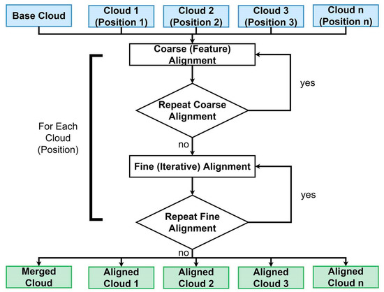
Figure 3.
Workflow showing the inputs and outputs of the alignment. This algorithm outputs each of the individually aligned scan positions as well as a complete merged cloud. Additionally, a subsampled version of the merged cloud can be exported.
Alignment was, perhaps, the most difficult step of this workflow. This was due to the tendency of alignment algorithms (specifically the ICP algorithm) to converge into a local minimum. To reduce the effects of this problem, the option to repeat alignment steps was added. This was done in order to “shake” the alignment out of the local minima by repeating the alignment step with slightly altered parameters. It was observed that individual dates aligned slightly differently depending on the presence of temporary obstructions (e.g., cars, snow, vegetation) and differences in scanning conditions. By repeating the scanning steps (once for the coarse alignment and four times for the fine, iterative alignment) the effects of these difference were reduced. The sampling size was reduced by 20% for each repeated coarse alignment and 10% for each repeated iterative alignment. Table 2 provides parameters used in both alignment algorithms. The parameters were chosen by repeatedly running the alignment steps for data with different degrees of subsampling and examining the results. Based on the range of acceptable values, a value that was centered between the extremes was chosen. Examining a large range of degrees of subsampling (achieved by varying the voxel grid size) ensures that for this type of setup, where the scanner is relatively close to the slope (e.g., for highway adjacent slopes) and a similar initial voxel filter is used, the parameters and algorithms should easily be adapted with reasonable adjustment to parameters.
Table 2.
Parameters used for alignment algorithms.
2.4.1. Coarse Alignment
A coarse alignment was implemented because the ICP requires an accurate initial estimate of the transformation parameters to achieve convergence. This was necessary since ICP has a tendency to converge to a local minimum [56,57]. As a result, it was advantageous to give an initial course alignment that was based upon features or picking point pairs, that the ICP could then further improve upon.
The first stop of the course alignment was segmentation to the general area of interest. Segmentation required that the positions of the point clouds be known a priori; however, since the acquisition system was not static, the initial position of the raw point cloud was not guaranteed. To account for this, the centroid of the scan position’s point cloud and the base model were collocated. This was not necessary for the alignment, but it allowed for segmentation of the point clouds to a rough area of interest, even though the initial location of scan positions in space was unknown.
The next step of the coarse alignment was to prepare the point clouds for keypoint calculation. Keypoints are a subset of points from a point cloud that are located in descriptive regions (often on corners and along edges). These keypoints are used to align the point cloud based upon geometrically distinct regions [55]. Useful keypoints were positioned along the edges and corners of structures, while poor keypoints were in locations with nonunique geometries (e.g., the center of a plane). This preparation included filtering noise using an SOR filter, subsampling with a voxel grid filter and computing the normals for all of the points with a normal radius of three meters. The coarse alignment was performed using keypoints and feature histograms. 3D keypoints were calculated using an Intrinsic Shape Signature (ISS) keypoint detector (ISSKeypoint3D) [55]. This method created a view-independent representation of the point cloud. Each point was described by three characteristics: intrinsic reference frame (Fi), a 3D shape feature and an intrinsic shape signature (Si). These values were all computed within the algorithm and were influenced by the point cloud’s point spacing, normals and a parameter that defined the size of the 3D shape features (Feature Size in Table 2). Once the keypoints were calculated, the Fast Point Feature Histogram (FPFH) used them as inputs to create feature descriptors for each keypoint. The feature size parameter is used to determine how far around the keypoint the algorithm searches for points in order to calculate descriptors for the feature. Since this is describing large-scale features, the feature radius must be large (approximately 5–10 times the point spacing after subsampling). While it is possible to simply pass the keypoints onto the rejection algorithm and use that to generate correspondences, the FPFH features are highly advantageous in that they are orientation invariant and reliable over a range of scales [56]. This is important since point clouds from other slopes will undoubtedly have different feature orientations (resulting from jointing and rock properties) and scales (resulting from scanner acquisition parameters and distance between the scanner and the slope). This algorithm is susceptible to variations in point density, which highlights the importance of performing subsampling that creates a near constant point density for the cloud prior to alignment.
Rejection of the keypoint descriptors was performed using Random Sample Consensus (RANSAC) [57,59]. The primary user-defined parameter in this step was the inlier distance (see Table 2). This denoted the distance after which a point would be determined an outlier. Since at this point in the workflow the clouds were only preliminarily aligned by their centroids, the inlier had to be relatively large. If the inlier was too small, then all of the correspondences were rejected.
2.4.2. Fine (Iterative) Alignment
Iterative closest point (ICP) alignment was used to further reduce the root mean square error (RMSE) between the scans, following the coarse alignment. There have been many variations of the ICP alignment algorithm developed since its introduction in 1991 [42,58]. However, the standard procedure includes the following steps:
- Choice of correspondence pair points that can be used to relate the two point clouds.
- Rejection of correspondence pairs points that do not match given criteria.
- Determination of the error corresponding to the pairs of points following transformation.
- Repetition until error is minimized below a threshold or until a stopping condition is satisfied.
First, normals were computed based on the smaller uniform sampling size used in this step of the alignment (Table 2). Then, correspondence pairs were calculated. A correspondence pair matches points from the two point clouds based upon geometric (e.g., normal) and visual (e.g., color) properties. PCL provides correspondence estimation based upon the normal of the two point clouds, called normal shooting, which finds points in a secondary cloud closest to the normal of a point in the primary cloud. While there were other ways to capture correspondences, it has been shown that using normal shooting will give better results for clouds that were initially not close [60]. This ensures that, even if the rough alignment leaves considerable space (greater than 10 cm) between the two clouds, the correspondences will still be found.
Some correspondences may negatively impact the alignment. As a result, correspondence rejection must be used to remove unsuitable correspondences. The first rejection criteria implemented was rejection of points in multiple correspondence pair. This eliminated duplicate correspondences while retaining the correspondence with the smallest distance between point pairs. The second rejection criterion was based on the surface normals of the correspondence pairs. This rejection algorithm determined the angle between the normal for the points in a correspondence pair. If that angle was greater than a user-defined threshold, the correspondence pair was rejected. While an optimum match would have identical normal vectors, subtle changes in the slope and the scanning position and the chosen radius for normal calculation led to non-zero angles between the normals. More importantly, significant features (corners and edges of geometric features) will have a greater degree of curvature. As previously mentioned, keypoints were calculated for these types of areas; likewise, useful correspondences also pertain to these types of areas. He et al. [61] found that on scale from 0o to 90o, points that correspond to a feature have a higher degree variance than points corresponding to a nonfeature. As a result, a higher threshold degree must be used to account for the keypoints having relatively large curvature, otherwise all correspondences will be rejected [57,61,62]. The final rejection criterion computed the median distance between points and enforced a user-defined threshold, which sets the number of standard deviations by which the pair distance could diverge from the median point distance. All correspondence pairs that were greater than a threshold of 1.3 times the standard deviation were rejected [63]. The convergence criteria used to stop the repeated iterations was mean square error (MSE). A mean square error less than 1E-6 m stopped the algorithm.
While RANSAC can be used as a rejector and was used as a rejector for the coarse alignment, it behaved inconsistently within the iterative alignment. The results were highly variable, due to the nature of RANSAC, in which a random subset of points is chosen to perform the operation. When RANSAC rejection was performed, even for the same cloud and set of parameters, the results varied greatly. The randomness of this method led to poor repeatability and accordingly RANSAC rejection was not used for the ICP alignment.
2.5. Classification
In order to isolate bedrock within the point cloud, the points had to be classified. Classification of the slope and removal of snow, talus and vegetation relied on a masking method implemented by Weidner et al. [64] (Figure 4). A template was created that denoted regions where bedrock, talus and vegetation were located on the slope. This mask, once created, was applied to all of the scans. Snow and ice were removed by thresholding the return intensity values. The return intensity scales and threshold values may change depending on the scanning system, but for the FARO Focus 3D × 330, which has a −2047 to 2048 intensity scale, a threshold of intensity below 500 corresponded well to snow and ice [64]. For example, bedrock in a winter scan had an average intensity of 1600, while the snow in the scan had an average intensity of −550 with some points with return intensities as low as −1359.
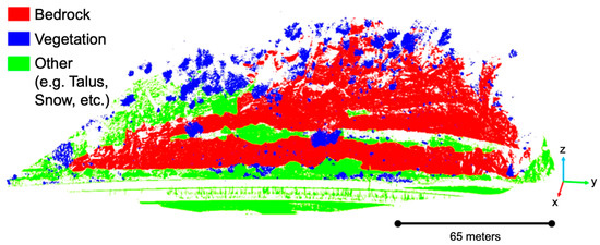
Figure 4.
The mask used to classify the Glenwood Springs study site. The mask will also label regions outside of the area of interest as “other”. This removed any outliers that were far from the slope. The mask was three dimensional, so vegetation that was isolated in front of the slope (e.g., free-standing trees and shrubs) was removed, while the bedrock behind remained. At this view angle, those objects may not clear, but they did occur on the slope.
The accuracy of this method depends on how quickly the characteristics of the slope change (e.g., how often new areas of the slope are newly vegetated, new snow catchments form, large rockslides drastically alter the slope). A large threshold radius (0.9 m) was used in order to account for these changes to the slope. This allowed points to be classified even if they were in a different location from the mask due to rockfall. Some areas of vegetation changed (e.g., due to growth) during the monitoring period, but they were largely removed by the noise filtering and cluster classification techniques (Section 2.3 and Section 2.9, respectively). For future years of data collection and processing, this mask will need to be assessed to analyze its quality and determine whether it needs to be edited to account for large changes in the slope.
2.6. Change Detection
Calculation of change between two point clouds was perhaps the most important step of this workflow. There are many algorithms designed for change detection, but the primary two involve a point-to-point (or mesh-to-mesh) nearest neighbor calculation [65] or a calculation along a surface normal [43,46]. The direction of change calculated is an important distinction between these two methods. A point-to-point calculation will calculate the distance between the two closest points in the data and reference clouds. This means that change will be calculated in the direction created by a vector between the two points. As a result, the change map does not show a specific direction of change. This is problematic when the two clouds have varying point densities. Noise in the calculation may be created by a calculation along the surface rather than outward or inward from the surface. Creating a mesh and using mesh-to-mesh distance will slightly reduce this problem, but this method is still not ideal for calculation of small changes, like those observed in this study, due to the introduction of interpolation error.
In contrast, a calculation along a surface normal will produce a change map of relative change along the normal. One of the first and most commonly used implementations of this change method is Multiscale Model-to-Model Cloud Comparison (M3C2) [43]. The M3C2 method is superior to nearest neighbor calculations in that it locally averages points in a manner that reduces error. It is also more robust for point clouds with missing points and variable point density [43]. One limitation of nearest neighbor calculations specific to rockfall analysis is the inability to differentiate whether change is occurring parallel or perpendicular to the slope. For example, in a case where the point cloud surface changes due to an oblong rockfall (where the area of change parallel to the slope is smaller than the change perpendicular to the slope) and a calculation is being performed for a point in the center of the area of change, a nearest neighbor algorithm will end up calculating a distance from the closest point that is parallel to the slope rather than perpendicular. In contrast, M3C2 searches for points along normal and averages, which means that the change perpendicular to the slope would be captured.
While this is a commonly used method, it is susceptible to error introduced by complex geometry (Figure 5). Methods have been proposed to reduce the effects of this with a user-defined range of cylinder lengths and user-defined maximum number of points within the cylinder. One method proposed by Williams et al. [24] defines a ranged cylinder search. Traditionally, the M3C2 algorithm begins searching for points at a distance (L) in the negative normal direction from the point and then extends forward until a distance (L) in the positive normal direction is achieved. Williams et al. [24] abbreviated this process by first extending the cylinder by 0.1 cm, then determining the number of points. If less than four points are found, the cylinder extends again. The maximum cylinder length and ranges of cylinder lengths to extend, are both user-defined variables.
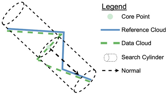
Figure 5.
An example of complex geometry, where the secondary surfaces would be captured along with the rockfall for an M3C2 cylinder extending in both the positive and negative normal direction.
The 4D filtering change technique presented in Kromer et al. [23] for deformation monitoring also computes distance along normals using a K-nearest algorithm; it relies on a maximum number of points (K), rather than a range of lengths. The change algorithm captures the K nearest neighbors in the secondary cloud and then filters all points that lie outside a perpendicular distance from the normal. A secondary step then averages calculated distances spatially and temporally to smooth out noise (i.e., 4D filtering step). The number of K points in the change algorithm and the number of nearest neighbors (NN) are defined by user input. For a cloud with high surface roughness, using a high K number is recommended to appropriately capture corresponding points in the secondary point cloud. However, testing this algorithm showed that it has a tendency to underestimate the change. In order to overcome this a large value of K must be specified (Section 3).
The algorithm proposed in this study builds upon both of these methods (Figure 6). It begins with the calculation of normals using single value decomposition. Normals pointed backwards into the slope are reversed. This was defined by an angle greater than 110 degrees between the normal and the preferential orientation, which is an optional input by the user. In this case a preferred orientation in the positive x-direction was used. However, the algorithm does allow for a dynamic calculation of the rock slope’s normal to use as the preferential orientation. The next step of the algorithm determined the calculation of the distance along each of these normals. An alteration to the M3C2 algorithm is proposed here. This method takes advantage of M3C2′s ability to average the direction of change (whether positive or negative along the normal). The procedure includes two steps.
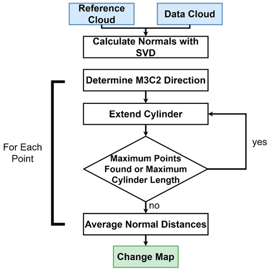
Figure 6.
Overview of the change detection algorithm.
- Determination of change direction (positive or negative along normal) using M3C2.
- Project the cylinder in the determined direction until K points have been found
The theoretical motivations behind these changes are twofold. First, determining a primary direction of change means that the cylinder is only projected in one direction. Thus, this means that the projection cylinder cannot intersect with planes in two different directions as shown in Figure 5. Second, the likelihood of intersecting more than one surface is reduced by stopping the cylinder projection once K points have been found. Discussion of the advantages of these changes is provided in Section 3.1 in the context of the obtained results.
The diameter of the nearest neighbor search used to calculate the normal should be 20–25 times the surface roughness of the point cloud, since uncertainty due to surface roughness in a normal calculation becomes negligible at that scale [43]. In order to capture the most detail, the projection cylinder must be as small as possible. However, while averaging the points within the cylinder reduces the effects of surface roughness, point density must still be considered. In order to capture as much change detail as possible, while still capturing multiple points to average the change values and reduce the effects of surface roughness, a projection cylinder between 5–10 times the point spacing was used. In this method, the maximum number of points could be dynamically calculated to correspond to the number of points found in the reference cloud within the defined cylinder radius. This allowed for the calculation to be purely dynamic, without requiring user input for the maximum number of points or a range of cylinder lengths. However, the maximum number of points could be overridden by the user. An example of the change algorithm applied to a four-month time period between October 2019 and February 2019 is shown in Figure 7.
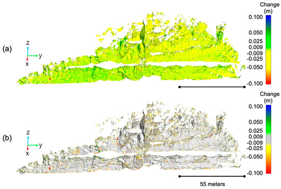
Figure 7.
Change detection using the proposed method for a four-month period (10-13-2018 to 02-18-2019) at the Glenwood Springs study site. The scale bar shows all change greater than 0.1 m and less than −0.1 as blue and red, respectively; as such, large changes typically correspond to the accumulation or loss of material rather than continuum slope deformation. (a) Change map showing deformation and rockfall; (b) greyed out. Small rockfalls are visible across the slope. A distinct rockfall is located in the far left corner with a volume of approximately 0.84 m3.
2.7. Clustering
After the change maps for each of the time periods were calculated, the volumes associated with rockfall events needed to be identified and clustered. First, the change cloud was filtered by removing all points with change below the limit of detection. To identify rockfall the change calculation was performed in two directions: forward, calculating change from the earlier date to the later date and reverse, calculating change from the later date to the earlier date. This represented both the front and back surface of the rockfall. To get these surfaces associated with slope degradation rather than accumulation, all positive change was removed for the forward calculation and all negative change was removed for the reverse calculation. After this, the two clouds (positive and negative change) were merged. Then, clustering was performed with the density-based spatial clustering of applications with noise (DBSCAN) algorithm [66,67,68]. The clustering code written for this study addresses one of the largest shortcomings of the M3C2 algorithm implemented in MATLAB. DBSCAN uses a radius (ε), nearest neighbor search to examine points and determine if the number of points found is at or above the user defined threshold (mp) and can be considered a cluster. Then, the process is repeated for each found point and this process is repeated until a point with a surrounding density less than mp is found. The code stores all of the indices of all of the points leading to redundancy and an exponential increase in memory use. For the large (multi-million point) clouds examined in this study, the memory usage would overload the computer. This was optimized by adding steps to check whether points had already been classified (as noise or a cluster) to reduce redundancy in the code. This made the memory usage and the computation time more efficient.
In order to capture small volumes (<0.001m3) while reducing the possibility for large volumes to split, “looser” parameters were chosen for clustering (ε = 0.1 m; mp = 35). The minimum number of points was chosen based upon the average point spacing within the volume created by a sphere with a radius equal to epsilon. Visual examination of the point cloud found that the majority of 0.1 m × 0.1 m × 0.1 m boxes in the bedrock contained more than 35 points. This means that any change in areas of this size could be expected to be clustered. This also resulted in many clusters being generated that corresponded to non-rockfall “clutter” (e.g., edges of vegetation, edges of snow, areas with higher alignment error), which had to be removed (Section 2.9).
2.8. Volume Statistics
A number of volume descriptors and statistics were calculated for each point cluster in order to separate rockfall from remaining clutter after clustering. The first statistic calculated was the primary, secondary and tertiary orthogonal axes of the cluster. There were a number of ways to determine the length along the primary axes, including, but not limited to, bounding box and adjusted bounding box [21]. While bounding box methods are commonly used [18,41], they have their limitations. A traditional bounding box method creates a three-dimensional box around the points with the minimum possible side lengths. The drawback of this method is its dependence on the cartesian coordinate axes. The box is created along the x, y and z axis, but a rockfall may not be naturally aligned to those axes. The adjusted bounding box method was created to overcome this limitation [21]. This method implements a single value decomposition to determine the orientation of the rockfall. Then, the bounding box is rotated so that the primary rockfall axis is aligned with the x-axis. Though the primary axis of the rockfall and the primary axis of the bounding box are now consistent, this method is still limited by the possible misalignment of the secondary and tertiary axes. Because of these limitations, a bounding box method was not used to determine the rockfall shape. Instead, principal component analysis (PCA), which has been used for other rockfall studies [40], was used to determine the primary, secondary and tertiary axes of the rockfall. From these, the lengths of the volume along its axes were calculated.
The next set of descriptors pertain to the number of points within the cloud and the volume. When comparing the number of points for a rockfall and patch of vegetation of the same 3D size, the number of points will often differ. While the points of a rockfall were located along the boundary of the object, the points for vegetation may be located on the boundary of the object and within the object. Because of this, the ratio of volume and total points was used in the classification of clusters. This is further explained in Section 2.9. The volume was calculated using the alpha shape process defined in Section 2.8.1. This value was used to compute the ratio (R) of the cloud by dividing the volume (V) by the number of points (Nr) corresponding to the rockfall (Equation (2)).
The other statistics calculated were related to the change. Specifically, the mean, maximum, minimum and average change were recorded to allow for simple analysis of the distribution of change within each cluster.
2.8.1. Shape Reconstruction
Shape reconstruction allows for a volume calculation from a set of points [13,66]. While there are other forms of volume reconstruction used in the literature (e.g., power crust) [20,48], alpha shape is most commonly used [18,40,44] and was the volume reconstruction algorithm used in this study. The concept of the alpha shape structure was proposed by Edelsbrunner and Mücke [47]. The alpha shape algorithm is controlled by an alpha radius. This defines that the Delauney triangulation that reconstructs the shape will have a circumcircle with a radius less than the alpha radius. The alphashape() function in MATLAB can theoretically be used to determine an appropriate radius for the calculation; however, tests with this method did not prove successful. In order to determine a threshold radius for a wide range of shapes, one-hundred rockfall volumes of varying sizes and shapes were tested. For each volume, a threshold radius was manually determined. This threshold radius was defined as the minimum radius that did not produce any holes within the shape. Figure 8 shows the influence of the alpha radius choice on shape reconstruction of a complex rock volume. This volume was represented by areas of continuous point coverage and a region that was blocked from the line of sight of the scanner. The occluded region created a large hole when a small alpha radius was used. This is an example of a complex situation where some regions of a rockfall are best modeled using a small radius and others are best modeled using a large radius. The maximum possible volume of this rockfall (4.83 m3) corresponds to a shape reconstruction with an infinite radius. The panels of Figure 8 show the effect of increasing alpha radius:
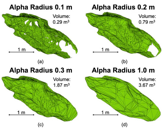
Figure 8.
Examples of shape reconstruction varying with the alpha radius (α). As the radius increased, the number of holes decreased, and the volume increased. (a) Volume reconstruction resulting from an alpha radius of 0.1 m; (b) Volume reconstruction resulting from an alpha radius of 0.2 m; (c) Volume reconstruction resulting from an alpha radius of 0.3 m; (d) Volume reconstruction resulting from an alpha radius of 1.0 m.
- Panel A: When the alpha radius is small, many holes appear resulting in an underestimation of the volume.
- Panel B: Increasing the radius decreases the number of holes and increases the volume estimate.
- Panel C: Holes have been eliminated with this, but some of the detail in the shape has been lost. This implies a threshold radius between 0.2 m and 0.3 m was suitable.
- Panel D: Too large of a radius results in complete deterioration of the shape.
For 100 rockfall point clusters, a range of volumes were calculated using alphashape(). Each volume calculated corresponds to an alpha radius between 0 m and 3 m. This resulted in an array of volumes for each rockfall point cloud. Plotting this range of volumes determined the solid lines plotted in Figure 9. A clear trend was visible. As the alpha radius increased and consequently the number of holes in the shape reconstruction decreased, there was a sharp increase in the calculated volume that approached an asymptote that defined the maximum volume.
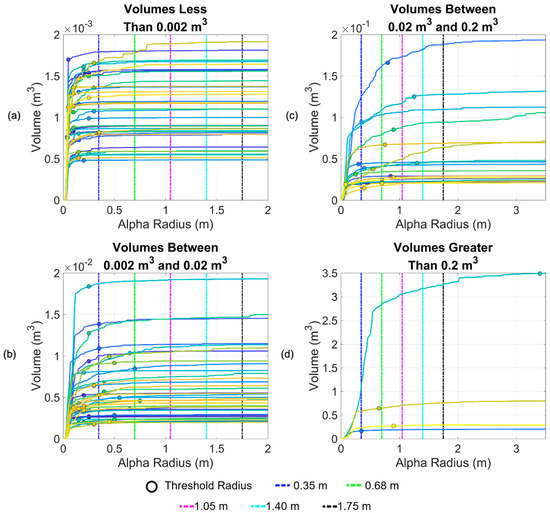
Figure 9.
Examination of volume curves for 100 rockfalls. Radii represented by the dashed lines correspond to the 10th–50th radius percentiles. The scales of figures (a,b) differ from the scales of figures (c,d), which allows the smallest and largest individual volumes to be visible in the latter two panels.
The threshold radius, which defined the minimum radius that created a shape reconstruction without any holes is denoted by a circle in Figure 9. The maximum radii that can be used to define a suitable alpha radius for a range of volumes are denoted by dashed lines in Figure 9. For example, for volumes whose maximum volume was less than 0.002 m3, a radius less than 0.35 m produces a good reconstruction. For volumes with a maximum volume between 0.002 m3 and 0.02 m3, a radius less than 0.68 m produces a good reconstruction.
As the rockfall volume increased, the threshold radii became less consistent. This was due to inconsistent point spacing. For larger volumes, it was much more likely that part of the volume would be out of view of the scanner due to occlusion. In terms of the reconstruction, this meant that some areas are well-defined by a small α and others required a large α to close holes. As a result, there was high variability in the threshold radius for the large volumes considered. Although a comprehensive solution to the alpha radius determination problem is beyond the scope of this work, our findings indicate that small volumes can be automatically estimated using a radius between 0.35 m and 0.68 m. A slope with drastically different rockfall characteristics may require a reproduction of this analysis to determine the relevant radii for volumes on that slope.
2.9. Cluster Classification
While some studies have implemented methods to differentiate points that are and are not related to rockfall, these algorithms are often applied prior to clustering [67]. This means that points are classified, but not the clusters that are meant to represent the rockfall volumes. Following clustering with DBSCAN, other workflows do not document how clusters are evaluated. This implies that either all of the clusters were automatically considered rockfall, or a manual validation process was performed. In this study, the goal was to filter out erroneous clusters automatically.
To reduce the initial amount of clutter, the clusters were filtered. The first filter was based upon a minimum number of points. This was set to be equal to the minimum points for the DBSCAN clustering to ensure no smaller clusters were included. The second filter relied on change occurring in both the forward and reverse direction. A physical rockfall would show change in both the forward and inverse change calculations. Cases where this might not occur include areas of temporary occlusion or edges of vegetation. This will result in an apparent change based upon a lack of points in one cloud. For example, a temporary obstacle would show up as 100% negative change with no points showing positive change in the reverse calculation. In order to filter out these cases, the percent difference between number of the positive and the number of the negative change points observed within a given cluster could not exceed a specified threshold (80%). Even with these filters (results shown in Figure 10), clutter was still included in the output clusters. This required classifying and filtering individual clusters based on their geometric properties.
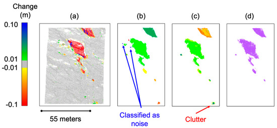
Figure 10.
Steps of the clustering algorithm applied to rockslide at a secondary slope. (a) The limit of detection is removed (greyed out in this image; (b) The clustering is performed, where noise is labelled as −1 (blue), while other clusters were given a unique number (unique color); (c) Clusters were preliminarily filtered to remove noise and clusters without change in both directions; (d) Rockfalls that were labelled manually, where one less cluster is present compared to Figure 10c.
Initial testing was performed using change results from aforementioned four-month period (October 2018 to February 2019) in order to include a large amount of rockfall with a wide range of sizes and shapes. Using the clusters, each individual rockfall was manually labeled as rockfall or clutter. The training set derived from a comparison between scans was 60 percent clutter and 40 percent rockfall. The features used to describe and classify each cluster are the following: number of points in the cluster, volume, ratio of volume and points (Equation (2)), mean change and standard deviation of change. Then, two different classification methods were used to classify the rockfall. Both methods used a training data set consisting of 70% of the manually classified rockfalls and a testing data set consisting of 30% of the rockfalls. The data were split using a random data partition.
The first method used was the generalized linear model regression (fitglm) in MATLAB [69,70]. This method creates a generalized linear model fit based upon variables within a table. All the cluster statistics were tested using a stepwise model, which determined the variables that were most important for determining the label. The most important cluster variables included number of points, density, volume, average change and the standard deviation of change. By specifying that the distribution of the model was binomial (rockfall or clutter), a logistic regression was performed.
The second method used was a bootstrapped random forest algorithm (TreeBagger) in MATLAB. In general, decision trees have the potential to overfit the data [71]. The bootstrap aggregation of multiple decision trees can be used to reduce this effect and each decision tree created uses a random sample of training instances and features [72,73].
Both methods output a score between zero and one that defined the probability of the cluster being a rockfall rather than clutter. Using a given threshold for this probability produced a unique number of false positive and false negative classifications. This information was used to determine the false positive rate (FPR) and false negative rate (FNR) (Equations (3) and (4)).
FPR and FNR are inversely proportional. As a lower probability threshold was used, the FNR decreased and the FPR increased. When creating the classifier, this inverse relationship allowed for a set of parameters to be identified that resulted in an equal FPR and FNR. To determine the probability threshold where the FNR and FPR curves intersected, a set of classifications with a range of probability thresholds were performed (Figure 11). The classification for each threshold value was repeated two hundred times in order to limit the influence of the random partition on the resulting classification. The results of these two hundred repetitions were recorded in the form of a boxplot. The probability threshold selected was the point where the median FNR and FPR values intersected. This was 0.475 for the generalized linear model (GLM) method and 0.325 for the random forest method.
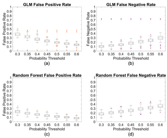
Figure 11.
Examining probability thresholding for the two methods. (a) FPRs for the GLM classifier; (b) FNRs for the GLM classifier; (c) FPRs for the random forest classifier; (d) FNRs for the random forest classifier.
The random forest decision tree was ultimately considered superior to the linear model in two respects. First, the run time of the random forest is much shorter (faster computational speed), than that of the linear model. Second, although the FNRs were similar for the two models, the random forest classifier produced an overall lower FPR. The random forest classifier was further tested to understand the effects of the training data quantity and volumetric distribution on the resultant classification. This showed that the distribution of the training data will have an impact on the classified data. A volumetric distribution matching that of the data to be classified produced the best results.
3. Results
3.1. Results of the Workflow Applied to the Glenwood Springs Slope
The proposed workflow was used, in conjunction with manual validation to construct a rockfall database and cumulative magnitude frequency curves for the Glenwood Springs slope. The time efficiency is an incredibly important aspect of this work. While there are some manual, one-time processes required to setup the workflow (e.g., tuning parameter and defining the boundary of the area of interest in 3D space) the automated alignment algorithm reduced what would be a manual process taking multiple hours to an automated process that can be run in the background, including repetitions of the individual alignment types (coarse and fine). While the modified M3C2 method did not reduce computational time of the algorithm, it did show a reduction in noise/outlier change when compared to previous algorithms.
The change algorithm was tested with synthetic data and real rockfall data. Figure 12 illustrates a comparison between the proposed method, here called “modified M3C2”, the traditional M3C2 method [43] and the K-nearest change algorithm implemented in the 4D filtering algorithm proposed by Kromer et al. [23]. First, the modified method was compared to M3C2 using synthetic data (see Figure 12a). Two planes with noisy points randomly generated around them were populated with varying point densities and distances. The modified method reduced the RMSE in this calculation. Then, the change algorithm was tested with a real rockfall volume. Manual measurements were used to determine the theoretical change limits (approximately 0 m to 1 m). The results of the change calculation revealed interesting trends in each method tested. As expected, M3C2 tended to include larger values of change due to intersection of the search cylinder with multiple surfaces. Problems with the K-nearest method were observed for oblong volumes. Since the nearest neighbors were found and then those nearest neighbors were filtered to the extent of the defined cylinder, a low value of K (e.g., K was equal to 10 for the modified M3C2 calculation) resulted in an undefined change calculation for the majority of the volume displayed in Figure 12. A high number of K neighbors (>3000) were required to appropriately capture points along the normal that were parallel to the slope rather than perpendicular to the normal direction. While the change calculation reduced outliers when compared to M3C2, the computation time of the K-nearest method was over 80% greater than that of the modified M3C2 method. A proposed modification to the K-nearest method applied in Kromer et al. [23] would be to change the order of operations to first constrain the region within a cylinder and then calculate the nearest neighbors within the cylinder to improve efficiency of the algorithm. Overall, the modified M3C2 method was able to capture this complex rockfall volume a reduce the number of outliers in the change calculation.
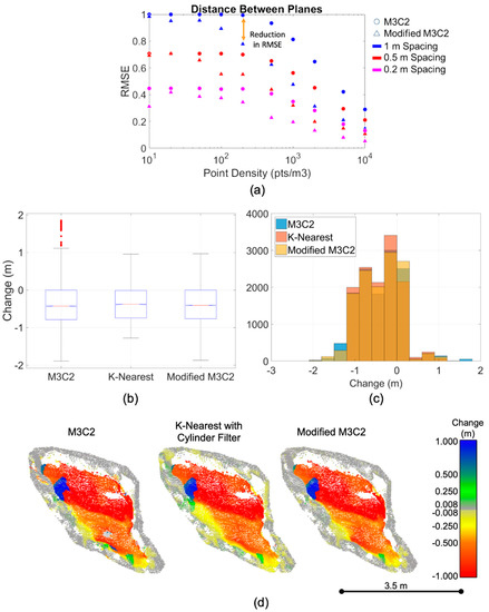
Figure 12.
Comparison of M3C2 and the modified method using synthetic data; (a) Results of comparing M3C2 and the modified method proposed for a synthetic plane; (b) Change calculations for the rockfall shown in Figure 12d as represented by M3C2, the nearest neighbor change method proposed by Kromer et al. 2017 (“K-Nearest”), where K = 3000 and the proposed modified M3C2 method. The modified M3C2 results have fewer outliers; (c) Change calculations for the rockfall shown in Figure 12d, which demonstrate fewer outliers resulting from the modified method; (d) Comparison of change calculated for a rockfall. Change below the limit of detection or undefined is shown in grey.
The automated classification of clusters reduced error in the database, where error was considered the number of clusters mislabeled as rockfall in the database. The final clutter filter (random forest with 0.325 probability threshold and no volume threshold for training) was applied to clusters generated over a two-year period for which a validation set was manually developed. It should be noted that the probability threshold was chosen at a point where the FNR and FPR were equal for the training set. This means that when applied to another set of data (in this case over a two-year period), the FNR and FPR resulting from the classification were not guaranteed to be exactly equal. The FNR and FPR for this classification were 28% and 17%, respectively. Figure 13 shows MCF curves generated for the small two-year test database. Rockfall on the slope studied are generally not very large and the workflow was optimized to be able to catch very small volumes in order to understand rockfall patterns over time (<0.001 m3). As a result, much of the error (in the form of clutter) is concentrated in the smaller volumes (<0.01 m3). Such extremely small volumes may not be relevant for other studies. As a result, the FNR and FPR were also calculated for thresholder ranges of volumes. When the volumes were thresholded to remove volumes less than 0.003 m3, the FNR and FPR become 20% and 19% respectively. When the volumes were thresholded to remove volumes less than 0.01 m3, the FNR and FPR become 14% and 25%, respectively. Despite the slightly higher FNR and FPR, the total error, as a percentage of clutter within rockfall database, was reduced from 63% to 20% for the testing data. This algorithm was later applied to a larger database of scans for the Glenwood Springs site that consisted of 40 scans. For this larger database, using the automatic cluster classification algorithm reduced the amount of clutter by 69%.
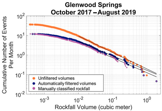
Figure 13.
Comparison of the magnitude-frequency curves generated from an unfiltered set of volume, an automatically filtered set of volumes and a manually filtered set of volumes.
This classification was shown to overpredict small volumes and underpredict larger volumes. Depending on the parameters chosen for the DBSCAN clustering and the size of the rockfall, there is also the possibility that some rockfall were split into multiple clusters, resulting in misclassification. Because of this, some volumes were flagged for manual analysis. Volumes were flagged for manual validation if they met any of the following criteria:
- The maximum cluster volume (corresponding to the infinite alpha radius) was greater than 0.2 m3.
- The centroid of the cluster was within a threshold distance from the centroid of another cluster.
The first flag ensured that the correct alpha radius was chosen for the volume calculation and that no large volume was incorrectly classified as clutter. The second flag accounts for the case where one rockfall is split into multiple clusters. To determine if two clusters were within a certain threshold distance, the following procedure was used:
- calculate the distance between cluster centroids.
- select the larger of the primary axis lengths for each of the clusters.
- if the distance between centroids is smaller than the larger of the primary axis lengths, the clusters were flagged for manual validation.
3.2. Results of the Workflow Aplied to a Secondary Slope
To further demonstrate the general applicability and adaptability of the proposed workflow, it was applied to a secondary slope. This slope is also located along a highly trafficked section of I-70 approximately 40 km west of Denver, Colorado, in an area called Floyd Hill. The slope is composed of feldspar and biotite ridge gneiss with conformable layers that are observed to be ½ inch to several feet thick [74,75]. The steepness of the slope, which is greater than 70 degrees and the foliation of the gneiss make rockfall frequent on this slope. Though only separated by approximately 142 miles along I-70, this slope’s characteristics are noticeably different from the Glenwood Springs slope. The Glenwood Springs site is dominated by relatively smooth surfaces, as a result of the megacrystic granite that makes up the site. In contrast, the Floyd Hill site appears rough and flaky. The high percentage of biotite in the gneiss that makes up the Floyd Hill site, creates sharp overhangs that are persistent across the slope; these types of sub horizontal overhangs were not common at the Glenwood Springs site.
Lidar scans collected for this site used the same scanner and setup as that used for the Glenwood Springs site, with the addition of a fourth scanning position. It should be noted that the distance between the slope and the scanner was greater; while the distance at the Glenwood Springs slope was approximately 30 m, the distance at the Floyd Hill site was greater than 50 m. The mean point density was greater than 2000 points per cubic meter and the distance between points in regions directly in front of the scanner, with the highest point density, was approximately 0.020 m. The proposed workflow was used to create a rockfall database for a 178-day period between 3 March 2019, and 31 August 2019 (Figure 14).
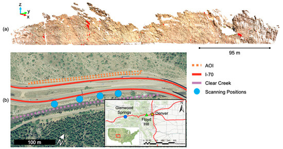
Figure 14.
(a) A point cloud representation of the Floyd Hill slope with the rockfalls occurring on the slope between 3 March 2019 and 31 August 2019 highlighted in red; (b) Site map showing the slope and scanning positions.
The workflow was applied to this slope with only minor alterations to algorithm parameters (Table 3). Even with so few changes to the parameters, a low limit of detection (1.8 cm) was achieved. For the cluster filtering step, although using the training data from Glenwood Springs produced an error of less than 10% (where error is the percentage of clusters whose label did not agree with the manual classification), we also created a set of training data that was specific to the Floyd Hill slope. This training data set was comprised of 1596 clusters from the Floyd Hill slope and used the same metrics and volume statistics to classify clusters. Rerunning the code used to generate Figure 11, the probability threshold where the FNR and FPR intersected was found to be 0.104. Using this dataset and the proposed random forest classifier, the error in the database was less than 6.5%, with no false negative labels for a volume greater than 0.05 m3. The results of this applied to the database are shown in Figure 15.
Table 3.
Comparison of parameters for the Glenwood Springs and Floyd Hill slopes.
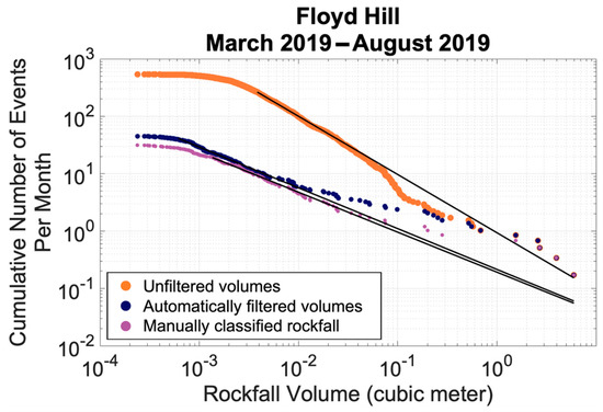
Figure 15.
Comparison of the magnitude-frequency curves generated for the Floyd Hill slope.
4. Discussion
The primary goal of this study was to create a comprehensive workflow that performs all point cloud processing steps for rockfall analysis from alignment to generation of geometric statistics and descriptors for a rockfall database. A secondary goal of this study was to address some of the gaps in knowledge left by workflows in other studies.
Previous studies have improved the M3C2 algorithm [23,24]. The proposed modified method builds upon these and reduces error in the calculation by limiting the extent and direction of the cylinder projection. This was shown to reduce error in calculations of change between two synthetic planes (Figure 12a) as well as for rockfall volumes (Figure 12b–d). One limitation of this method is the dependence on the normal direction. As with M3C2, if the normal is oriented incorrectly, then the change cannot be accurately calculated. Another limitation is reduced computational speed. Because the change direction is first calculated with the base M3C2 method, this algorithm is no faster than M3C2.
During the development of this workflow, the order of operations was observed to be very important. This was especially true for the change calculation algorithm. Artifacts of temporary objects were observed in cases where the classification was performed subsequent to the change calculation. If the number of points used in the calculation is limited to a defined number of nearest neighbors, then filtering to a shape (e.g., a cylinder) must be performed prior to determining the closest points. Otherwise, although points lie within the defined shape, they may not be considered since they are not the absolute nearest points. Another observation was the relationship between rockfall size and trends in alpha radii. While an appropriate alpha radius for small rockfalls could easily be defined by a maximum radius, as the volume increased, the appropriate radii could not be defined by a simple relationship and it was more difficult to close holes in the reconstructions without losing details regarding certain parts of the reconstruction. Other algorithms have been able to perform reconstruction without having to consider holes (e.g., power crust) [48]; however, like the alpha shape algorithm, there are user defined parameters that must be determined. It should be noted that Bonneau et al. [45] presents an alternative method for automating reconstruction parameter selection.
Another previous gap in knowledge addressed in this study was the procedure for use of points cluster after they have been obtained by DBSCAN. Other studies that have used this clustering algorithm [18,20,40,44], but do not indicate how erroneous clusters were excluded (or managed). Whether these values were included along with the rockfall or manually removed has implications for both the magnitude-frequency curve (Figure 13 and Figure 15) and the processing time. This novel cluster classification implements machine learning algorithms to automatically classify point clusters. Since the statistics used to describe the clusters (change, point density, etc.) are not specific to an acquisition method, this proposed algorithm could be applied to projects that implement terrestrial photogrammetry rather than lidar. Initial results for the Glenwood Springs site showed that error (as a percentage of rockfall whose label does not agree with the manual label) was reduced by 68% when the automatic classifier was applied to the clusters.
The results of the workflow applied to the secondary Floyd Hill rock slope, show that this workflow is adaptable to other slopes even with different distances between the slope and the scanner and different rock properties. Comparing the site positions, the distance between the scanner and slope at the Floyd Hill site was almost double that of the Glenwood Springs site. The megacrystic granite at the Glenwood Spring site resulted in relatively smooth surfaces disrupted by joints. In contrast, the foliation of the gneiss at the Floyd Hill site gives the appearance of a very rough, flaky surface. This was shown in the local surface roughness as well, for which the Floyd Hill sites was higher. Despite these differences between the slopes, the proposed workflow was demonstrated to perform well on both with nearly identical processing parameters.
While the initial subsampling radius was increased slightly from the Glenwood Springs case to the Floyd Hill case (see Table 3), the alignment algorithm was applied without any parameter changes and resulted in a low limit of detection. Likewise, applying the original training data set and cluster classifier resulted in less than 10% error. Creating a training dataset specific to the Floyd Hill site further reduced the error to less than 6.5%. Though a site-specific training dataset was created, the time it takes to manually label a small subset of clusters is minimal compared to manually classifying thousands of clusters. It should be noted that the kink in the magnitude cumulative-frequency curve (volumes greater than 0.1 m3) is not an artifact; it is related to a large rockslide event that occurred during a thunderstorm in June of 2019.
The total error in the automated classifier (Figure 13 and Figure 15) is greatest for volumes that are very small (<0.001 m3) and for mid-range volumes (0.001–0.01 m3). This can be explained as follows. First, the high temporal resolution of this dataset makes it possible to capture clusters that are small (<0.001 m3). In order to create these small clusters, the DBSCAN clustering parameters must be conservative (e.g., a number of minimum points that corresponds to the average point density rather than the highest available point density). This increases the probability of clustering points that are not part of a rockfall. As a result, there is a high quantity of clutter in the database for small and mid-range volumes (<0.01 m3). Second, the workflow was designed to be conservative, in that it will allow more false positive classifications so that few false negative classifications occur. For the secondary site tested, less than 2% of the total error was a result of false negative classifications. When examining relative error, the error is greatest for mid-range volumes (0.001–0.01 m3) and large volumes (>0.1 m3), which can be explained as follows. First, as previously mentioned, the workflow was designed to be conservative; thus, there is a greater chance of false positive classifications. There were no false negative classifications for volumes greater than (0.03 m3). Second, the volumes of rockfalls in the database are approximately lognormally distributed. This is also true for the training data set, which was created using rockfall data from the same slope. This means there is a limited number of samples of rockfalls with volumes greater than 0.01 m3 in the training data. In future applications, training data could be curated to focus on volume ranges of interest for a given application.
While there is a notable degree of error associated with this classifier, it is important to note that the goal of developing this method was to reduce the manual classification of rockfall, rather than remove all quality control from the process of creating a rockfall database. To further improve the accuracy of the database, without greatly increasing the manual workload, the positive classifications could be quality-controlled to remove false positive classifications. Manual classification of the positively labelled clusters substantially decreases the error. For the Floyd Hill site, the error would decrease to less than 2% error. However, even with this manual classification, the total manual effort is still a 93% decrease when compared to manually classify every cluster. Applications of this workflow may implement varying amounts of manual classification depending on the error tolerance of the study and the amount of time available for manual classification.
The proposed workflow was designed to construct a rockfall database in order to better understand rockfall frequency and rate. Because of this, a goal of the automated classifier was to also reduce error in the a and b constants for the MCF curve. When applied to the secondary slope, the percentage difference in the estimated MCF fit constant a was reduced from 131.8% to 11.0% and the percentage difference for the MCF fit constant b was reduced from 37.2% to 2.0%. The database without any classification had significantly more false positive classifications (as all clusters are considered rockfall), which means that it forecasted a significantly higher frequency for large rockfalls when compared to the other two classified databases. For example, the frequency of a 10 m3 rockfall was forecasted to be approximately every 26, 19 and 11 months for the manually classified, automatically classified and full database MCF curves respectively.
There are other use cases where this workflow could be adapted for a monitoring system. For example, for a highway or railway monitoring system, which would only examine rockfalls that are cobble size (0.1 m3) or larger, this workflow could be used in conjunction with frequent data collection to alert relevant parties about a rockfall occurrence. At the Floyd Hill site, for volumes greater than 0.1 m3, the error in the database was less than 0.2%, with none of the error associated with false negative classifications. Since false positive results still occur at a relatively high rate for larger volumes, a positively classified cluster would need to be validated as a real rockfall. However, even with this manual classification of rockfalls identified by the classifier, the manual workload is greatly decreased. For example, if an alert system was set up for the Floyd Hill site, where alerts were given for all positive rockfall classifications greater than 0.1 m3, the manual workload would decrease by 77% when compared to manually classifying all clusters in that volume range.
There are some limitations to this process. While the goal of full automation is desirable, there must be some compromise between the amount of error allowed and the amount of automation. This is perhaps most clearly demonstrated in the clutter filtering algorithm. Full automation of the filtering meant that some number of false negative and false positive rockfalls resulted from the classification. This process resulted in more false positives for small volumes and more false negatives for the larger volumes. This, along with the importance of alpha radii for large volumes, made it important to introduce some manual validation in the workflow. This demonstrates the fact that, to a certain extent, there is a tradeoff between automation and accuracy.
5. Conclusions
Automating point cloud processing for the purpose of rockfall monitoring is a complex problem that requires an initial setup period, where parameters are tuned to account for geometry of the slope, scanning resolution and scanner limitations. This study proposes methods for expediting the choice of algorithmic parameters and proposes novel methods of automating steps that are normally manually performed. One potential area for future work is the application of this workflow to new sites. As demonstrated in this study, the workflow could be used to study the frequency of rockfalls by generating a rockfall database. As previously mentioned, some manual quality control will likely be necessary for studies that implement this workflow for monitoring or alert systems. However, the automatic classifier proposed in this study can significantly reduce the amount of manual work required. Furthermore, future studies could possibly improve the proposed classifier by adding new cluster descriptors as part of the training data. For example, a study with clusters that were extracted from photogrammetric point clouds, which provide higher quality color data than the TLS method used in this study, could include color as a descriptor in the machine learning classifier.
The following conclusions were derived from this study:
- Testing the new modified M3C2 change algorithm showed that limiting the extent of the cylinder projection can reduce error from capturing secondary surfaces.
- Application of the proposed workflow to a secondary slope shows that this workflow can easily be adapted and used to processes point cloud data for rock slopes with different characteristics (e.g., point spacing and rock type).
- The proposed machine learning algorithm can be used to provide a classification of volumes, but it is limited by the number and quality of training samples provided. The proposed classification method resulted in FNR and FPR values of less than 20% for the initially tested Glenwood Springs Site. This proposed method for labelling cluster can save hours of manual volume validation.
- When applied to the secondary Floyd Hill site and without updating the training data), the proposed machine learning algorithm reduced error (as a percentage of automatic labels that disagreed with the manual label) to less than 10%. When training data specific to the Floyd Hill site were used to classify clusters, the error was further reduced to less than 6.5%.
Author Contributions
H.S. developed the workflow and its code, co-acquired and co-analyzed the data, and wrote the manuscript. G.W. coordinated the project, co-analyzed the data, and revised the manuscript. R.K. contributed analysis tools, including code, and revised the manuscript. A.M. co-acquired the data and co-analyzed the Floyd Hill data. All authors have read and agreed to the published version of the manuscript.
Funding
This work was supported by the Colorado Department of Transportation (CDOT).
Data Availability Statement
Data are available upon request, subject to authorization by the Colorado Department of Transportation.
Acknowledgments
Luke Weidner and Brian Gray provided essential assistance acquiring lidar scans for this project.
Conflicts of Interest
The authors declare no conflict of interest.
References
- Telling, J.; Lyda, A.; Hartzell, P.; Glennie, C. Review of Earth science research using terrestrial laser scanning. Earth Sci. Rev. 2017, 169, 35–68. [Google Scholar] [CrossRef]
- Prokop, A. Assessing the applicability of terrestrial laser scanning for spatial snow depth measurements. Cold Reg. Sci. Technol. 2008, 54, 155–163. [Google Scholar] [CrossRef]
- Corripio, J.G.; Durand, Y.; Guyomarc’h, G.; Mérindol, L.; Lecorps, D.; Pugliése, P. Land-based remote sensing of snow for the validation of a snow transport model. Cold Reg. Sci. Technol. 2004, 39, 93–104. [Google Scholar] [CrossRef]
- Deems, J.S.; Painter, T.H.; Finnegan, D.C. Lidar measurement of snow depth: A review. J. Glaciol. 2013, 59, 467–479. [Google Scholar] [CrossRef]
- Rosser, N.J.; Petley, D.; Lim, M.; Dunning, S.; Allison, R.J. Terrestrial laser scanning for monitoring the process of hard rock coastal cliff erosion. Q. J. Eng. Geol. Hydrogeol. 2005, 38. [Google Scholar] [CrossRef]
- Grayson, R.; Holden, J.; Jones, R.R.; Carle, J.A.; Lloyd, A.R. Improving particulate carbon loss estimates in eroding peatlands through the use of terrestrial laser scanning. Geomorphology 2012, 179, 240–248. [Google Scholar] [CrossRef]
- Nagihara, S.; Mulligan, K.R.; Xiong, W. Use of a three-dimensional laser scanner to digitally capture the topography of sand dunes in high spatial resolution. Earth Surf. Process. Landf. 2004, 29, 391–398. [Google Scholar] [CrossRef]
- Wang, W.; Zhao, W.; Huang, L.; Vimarlund, V.; Wang, Z. Applications of terrestrial laser scanning for tunnels: A review. J. Traffic Transp. Eng. (Engl. Ed.) 2014, 1, 325–337. [Google Scholar] [CrossRef]
- Jaboyedoff, M.; Oppikofer, T.; Abellán, A.; Derron, M.H.; Loye, A.; Metzger, R.; Pedrazzini, A. Use of LIDAR in landslide investigations: A review. Nat. Hazards 2012, 61, 5–28. [Google Scholar] [CrossRef]
- Abellán, A.; Vilaplana, J.M.; Calvet, J.; Garcia-Sellés, D.; Asensio, E. Rockfall monitoring by Terrestrial Laser Scanning—Case study of the basaltic rock face at Castellfollit de la Roca (Catalonia, Spain). Nat. Hazards Earth Syst. Sci. 2011, 11, 829–841. [Google Scholar] [CrossRef]
- Kromer, R.; Walton, G.; Gray, B.; Lato, M.; Group, R. Development and optimization of an automated fixed-location time lapse photogrammetric rock slope monitoring system. Remote Sens. 2019, 11, 1890. [Google Scholar] [CrossRef]
- Oppikofer, T.; Jaboyedoff, M.; Blikra, L.; Derron, M.H.; Metzger, R. Characterization and monitoring of the Åknes rockslide using terrestrial laser scanning. Nat. Hazards Earth Syst. Sci. 2009, 9, 1003–1019. [Google Scholar] [CrossRef]
- Olsen, M.J.; Wartman, J.; McAlister, M.; Mahmoudabadi, H.; O’Banion, M.S.; Dunham, L.; Cunningham, K. To fill or not to fill: Sensitivity analysis of the influence of resolution and hole filling on point cloud surface modeling and individual rockfall event detection. Remote Sens. 2015, 7, 12103–12134. [Google Scholar] [CrossRef]
- Lim, M.; Petley, D.N.; Rosser, N.J.; Allison, R.J.; Long, A.J.; Pybus, D. Combined digital photogrammetry and time-of-flight laser scanning for monitoring cliff evolution. Photogramm. Rec. 2005, 20109–20129. [Google Scholar] [CrossRef]
- Abellán, A.; Calvet, J.; Vilaplana, J.; Blanchard, J. Detection and spatial prediction of rockfalls by means of terrestrial laser scanner monitoring. Geomorphology 2010, 119, 162–171. [Google Scholar] [CrossRef]
- Hungr, O.; Evans, S.G.; Hazzard, J. Magnitude and frequency of rock falls and rock slides along the main transportation corridors of southwestern British Columbia. Can. Geotech. J. 1999, 36, 224–238. [Google Scholar] [CrossRef]
- Hungr, O.; McDougall, S.; Wise, M.; Cullen, M. Magnitude–frequency relationships of debris flows and debris avalanches in relation to slope relief. Geomorphology 2008, 96, 355–365. [Google Scholar] [CrossRef]
- van Veen, M.; Hutchinson, D.; Kromer, R.; Lato, M.; Edwards, T. Effects of sampling interval on the frequency—Magnitude relationship of rockfalls detected from terrestrial laser scanning using semi-automated methods. Landslides 2017, 14, 1579–1592. [Google Scholar] [CrossRef]
- Santana, D.; Corominas, J.; Mavrouli, O.; Garcia-Sellés, D. Magnitude–frequency relation for rockfall scars using a Terrestrial Laser Scanner. Eng. Geol. 2012, 145–146, 50–64. [Google Scholar] [CrossRef]
- Benjamin, J.; Rosser, N.J.; Brain, M.J. Emergent characteristics of rockfall inventories captured at a regional scale. Earth Surf. Process. Landf. 2020, 45, 2773–2787. [Google Scholar] [CrossRef]
- Bonneau, D.; Hutchinson, D.; Difrancesco, P.-M.; Coombs, M.; Sala, Z. 3-Dimensional Rockfall Shape Back-Analysis: Methods and Implications. Nat. Hazards Earth Syst. Sci. 2019, 19, 2745–2765. [Google Scholar] [CrossRef]
- De Vilder, S.J.; Rosser, N.J.; Brain, M. Forensic analysis of rockfall scars. Geomorphology 2017, 295, 202–214. [Google Scholar] [CrossRef]
- Kromer, R.A.; Abellán, A.; Hutchinson, D.J.; Lato, M.; Chanut, M.A.; Dubois, L.; Jaboyedoff, M. Automated Terrestrial Laser Scanning with Near Real-Time Change Detection-Monitoring of the Séchilienne Landslide. Earth Surf. Dyn. 2017, 5, 293–310. [Google Scholar] [CrossRef]
- Williams, J.; Rosser, N.J.; Hardy, R.; Brain, M.; Afana, A. Optimising 4-D surface change detection: An approach for capturing rockfall magnitude–frequency. Earth Surf. Dyn. 2018, 6, 101–119. [Google Scholar] [CrossRef]
- Eltner, A.; Kaiser, A.; Abellan, A.; Schindewolf, M. Time lapse structure-from-motion photogrammetry for continuous geomorphic monitoring. Earth Surf. Process. Landf. 2017, 42, 2240–2253. [Google Scholar] [CrossRef]
- Kromer, R.; Hutchinson, D.; Lato, M.; Gauthier, D.; Edwards, T. Identifying rock slope failure precursors using LiDAR for transportation corridor hazard management. Eng. Geol. 2015, 195, 93–103. [Google Scholar] [CrossRef]
- Rosser, N.J.; Lim, M.; Petley, D.; Dunning, S.; Allison, R. Patterns of precursory rockfall prior to slope failure. J. Geophys. Res. 2007, 112, F04014. [Google Scholar] [CrossRef]
- Kromer, R.; Lato, M.; Hutchinson, D.J.; Gauthier, D.; Edwards, T. Managing rockfall risk through baseline monitoring of precursors using a terrestrial laser scanner. Can. Geotech. J. 2017, 54, 953–967. [Google Scholar] [CrossRef]
- Stock, G.M.; Martel, S.J.; Collins, B.D.; Harp, E.L. Progressive failure of sheeted rock slopes: The 2009-2010 Rhombus Wall rock falls in Yosemite Valley, California, USA. Earth Surf. Process. Landf. 2012, 37, 546–561. [Google Scholar] [CrossRef]
- Royán, M.J.; Abellán, A.; Jaboyedoff, M.; Vilaplana, J.M.; Calvet, J. Spatio-temporal analysis of rockfall pre-failure deformation using Terrestrial LiDAR. Landslides 2014, 11, 697–709. [Google Scholar] [CrossRef]
- Delonca, A.; Gunzburger, Y.; Verdel, T. Statistical correlation between meteorological and rockfall databases. Nat. Hazards Earth Syst. Sci. 2014, 14, 1953–1964. [Google Scholar] [CrossRef]
- D’amato, J.; Hantz, D.; Guerin, A.; Jaboyedoff, M.; Baillet, L.; Mariscal, A. Influence of meteorological factors on rockfall occurrence in a middle mountain limestone cliff. Hazards Earth Syst. Sci. 2016, 16, 719–735. [Google Scholar] [CrossRef]
- Matsuoka, N.; Sakai, H. Rockfall activity from an alpine cliff during thawing periods. Geomorphology 1999, 28, 309–328. [Google Scholar] [CrossRef]
- Luckman, B.H. Rockfalls and rockfall inventory data: Some observations from surprise valley, Jasper National Park, Canada. Earth Surf. Process. 1976, 1, 287–298. [Google Scholar] [CrossRef]
- Pierson, L.A.; Vickle, R.V. Rockfall Hazard Rating System: Participants’ Manual. August 1993. Available online: https://trid.trb.org/view/459774 (accessed on 1 February 2020).
- Pierson, L.A.; Davis, S.A.; van Vickle, R. Rockfall Hazard Rating System: Implementation Manual. August 1990. Available online: https://trid.trb.org/view/361735 (accessed on 1 February 2020).
- Budetta, P.; Nappi, M. Comparison between qualitative rockfall risk rating systems for a road affected by high traffic intensity. Nat. Hazards Earth Syst. Sci. 2013, 13, 1643–1653. [Google Scholar] [CrossRef][Green Version]
- Santi, P.; Russell, C.P.; Higgins, J.D.; Spriet, J.I. Modification and statistical analysis of the Colorado Rockfall Hazard Rating System. Eng. Geol. 2009, 104, 55–65. [Google Scholar] [CrossRef]
- Chau, K.T.; Wong, R.H.C.; Liu, J.; Lee, C.F. Rockfall Hazard Analysis for Hong Kong Based on Rockfall Inventory. Rock Mech. Rock Engng 2003, 36, 383–408. [Google Scholar] [CrossRef]
- Carrea, D.; Abellán, A.; Derron, M.-H.; Jaboyedoff, M. Automatic Rockfalls Volume Estimation Based on Terrestrial Laser Scanning Data. In Engineering Geology for Society and Territory—Volume 2; Springer International Publishing: Cham, Switzerland, 2015; pp. 425–428. [Google Scholar]
- Williams, J. Insights into Rockfall from Constant 4D Monitoring; Durham University: Durham, UK, 2017. [Google Scholar]
- Besl, P.J.; McKay, N.D. A method for registration of 3-D shapes. IEEE Trans. Pattern Anal. Mach. Intell. 1992, 14, 239–256. [Google Scholar] [CrossRef]
- Lague, D.; Brodu, N.; Leroux, J. Accurate 3D comparison of complex topography with terrestrial laser scanner: Application to the Rangitikei canyon (N-Z). ISPRS J. Photogramm. Remote Sens. 2013, 82, 10–26. [Google Scholar] [CrossRef]
- DiFrancesco, P.-M.; Bonneau, D.; Hutchinson, D.J. The Implications of M3C2 Projection Diameter on 3D Semi-Automated Rockfall Extraction from Sequential Terrestrial Laser Scanning Point Clouds. Remote Sens. 2020, 12, 1885. [Google Scholar] [CrossRef]
- Bonneau, D.; Difrancesco, P.-M.; Hutchinson, D. Surface Reconstruction for Three-Dimensional Rockfall Volumetric Analysis. ISPRS Int. J. Geo-Inf. 2019, 8, 548. [Google Scholar] [CrossRef]
- Kromer, R.; Abellán, A.; Hutchinson, D.; Lato, M.; Edwards, T.; Jaboyedoff, M. A 4D Filtering and Calibration Technique for Small-Scale Point Cloud Change Detection with a Terrestrial Laser Scanner. Remote Sens. 2015, 7, 13029–13052. [Google Scholar] [CrossRef]
- Edelsbrunner, H.; Mücke, E.P. Three-dimensional alpha shapes. In Proceedings of the 1992 Workshop on Volume Visualization, VVS 1992, New York, NY, USA, 19–20 October 1992; pp. 75–82. [Google Scholar] [CrossRef]
- Amenta, N.; Choi, S.; Kolluri, R.K. The power crust. In Proceedings of the Symposium on Solid Modeling and Applications, Ann Arbor, MI, USA, 4–8 June 2001; pp. 249–260. [Google Scholar] [CrossRef]
- Mejfa-Navarro, M.; Wohl, E.; Oaks, S. Geological hazards, vulnerability, and risk assessment using GIS: Model for Glenwood Springs, Colorado. Geomorphology 1994, 10, 331–354. [Google Scholar] [CrossRef]
- Kirkham, R.M.; Streufert, R.K.; Cappa, J.A.; Shaw, C.A.; Allen, J.L.; Schroeder, T.J.I. Geologic Map of the Glenwood Springs Quadrangle, Garfield County, Colorado. 2009. Available online: https://ngmdb.usgs.gov/Prodesc/proddesc_94610.htm (accessed on 4 March 2020).
- Abellán, A.; Oppikofer, T.; Jaboyedoff, M.; Rosser, N.; Lim, M.; Lato, M. Terrestrial laser scanning of rock slope instabilities. Earth Surf. Process. Landf. 2014, 39, 80–97. [Google Scholar] [CrossRef]
- Rusu, R.; Marton, Z.C.; Blodow, N.; Dolha, M.; Beetz, M. Towards 3D Point cloud based object maps for household environments. Rob. Auton. Syst. 2008, 56, 927–941. [Google Scholar] [CrossRef]
- Gomez, C.; Purdie, H. UAV- based Photogrammetry and Geocomputing for Hazards and Disaster Risk Monitoring—A Review. Geoenviron. Disasters 2016, 3, 1–11. [Google Scholar] [CrossRef]
- Cheng, L.; Chen, S.; Liu, X.; Xu, H.; Wu, Y.; Li, M.; Chen, Y. Registration of Laser Scanning Point Clouds: A Review. Sensors 2018, 18, 1641. [Google Scholar] [CrossRef]
- Zhong, Y. Intrinsic shape signatures: A shape descriptor for 3D object recognition. In Proceedings of the 2009 IEEE 12th International Conference on Computer Vision Workshops, ICCV Workshops, Kyoto, Japan, 27 September–4 October 2009; pp. 689–696. [Google Scholar] [CrossRef]
- Rusu, R.; Blodow, N.; Beetz, M. Fast Point Feature Histograms (FPFH) for 3D registration. In Proceedings of the 2009 IEEE International Conference on Robotics and Automation, Kobe, Japan, 12–17 May 2009; pp. 3212–3217. [Google Scholar] [CrossRef]
- Holz, D.; Ichim, A.; Tombari, F.; Rusu, R.; Behnke, S. Registration with the Point Cloud Library: A Modular Framework for Aligning in 3-D. IEEE Robot. Autom. Mag. 2015, 22, 110–124. [Google Scholar] [CrossRef]
- Chen, Y.; Medioni, G. Object modeling by registration of multiple range images. In Proceedings of the 1991 IEEE International Conference on Robotics and Automation, Sacramento, CA, USA, 9–11 April 1991; pp. 2724–2729. [Google Scholar] [CrossRef]
- Fischler, M.A.; Bolles, R.C. Random sample consensus: A paradigm for model fitting with applications to image analysis and automated cartography. Commun. ACM 1981, 24, 381–395. [Google Scholar] [CrossRef]
- Rusinkiewicz, S.; Levoy, M. Efficient variants of the ICP algorithm. In Proceedings of the Third International Conference on 3-D Digital Imaging and Modeling, Quebec City, QC, Canada, 28 May–1 June 2001; pp. 145–152. [Google Scholar] [CrossRef]
- He, Y.; Liang, B.; Yang, J.; Li, S.; He, J. An Iterative Closest Points Algorithm for Registration of 3D Laser Scanner Point Clouds with Geometric Features. Sensors 2017, 17, 1862. [Google Scholar] [CrossRef]
- Pulli, K. Multiview registration for large data sets. In Proceedings of the 2nd International Conference on 3-D Digital Imaging and Modeling, Ottawa, ON, Canada, 4–8 October 1999; pp. 160–168. [Google Scholar] [CrossRef]
- Pomerleau, F.; Colas, F.; Ferland, F.; Michaud, F. Relative Motion Threshold for Rejection in ICP Registration. Springer Tracts Adv. Robot. 2010, 62, 229–238. [Google Scholar] [CrossRef]
- Weidner, L.; Walton, G.; Kromer, R. Classification methods for point clouds in rock slope monitoring: A novel machine learning approach and comparative analysis. Eng. Geol. 2019, 263. [Google Scholar] [CrossRef]
- Girardeau-Montaut, D.; Roux, M.; Marc, R.; Thibault, G. Change detection on points cloud data acquired with a ground laser scanner. In Proceedings of the ISPRS WG III/3, III/4, V/3 Workshop “Laser scanning 2005”, Enschede, The Netherlands, 12–14 September 2005; pp. 30–35. [Google Scholar]
- Guerin, A.; Rosetti, J.-P.; Hantz, D.; Jaboyedoff, M. Estimating rock fall frequency in a limestone cliff using LIDAR measurements. In Proceedings of the International Conference on Landslide Risk, Tabarka, Tunisia, 14–16 March 2013; Available online: https://www.researchgate.net/publication/259873223_Estimating_rock_fall_frequency_in_a_limestone_cliff_using_LIDAR_measurements (accessed on 6 April 2020).
- Tonini, M.; Abellán, A. Rockfall detection from terrestrial lidar point clouds: A clustering approach using R. J. Spat. Inf. Sci. 2013, 8, 95–110. [Google Scholar] [CrossRef]
- Ester, M.; Ester, M.; Kriegel, H.-P.; Sander, J.; Xu, X. A density-based algorithm for discovering clusters in large spatial databases with noise. In Proceedings of the KDD’96: Proceedings of the Second International Conference on Knowledge Discovery and Data Mining, Portland, OR, USA, 2–4 August 1996; Volume 3, pp. 226–231. Available online: http://citeseer.ist.psu.edu/viewdoc/summary?doi=10.1.1.121.9220 (accessed on 21 September 2019).
- Collett, D. Modelling Binary Data, 2nd ed.; CRC Press: Boca Raton, FL, USA, 2002. [Google Scholar]
- The Mathworks Inc. FitGLM. 2020. Available online: https://www.mathworks.com/help/stats/fitglm.html (accessed on 26 February 2020).
- Dietterich, T. Overfitting and Undercomputing in Machine Learning. ACM Comput. Surv. 1995, 27, 326–327. [Google Scholar] [CrossRef]
- The MathWorks Inc. TreeBagger. 2020. Available online: https://www.mathworks.com/help/stats/treebagger.html (accessed on 26 February 2020).
- Breiman, L. Random Forests. Mach. Learn. 2001, 45, 5–32. [Google Scholar] [CrossRef]
- Sheridan, D.M.; Reed, J.C.; Bryant, B. Geologic Map of the Evergreen Quadrangle, Jefferson County, Colorado. U.S. Geological Survey 1972. Available online: https://ngmdb.usgs.gov/Prodesc/proddesc_9606.htm (accessed on 27 February 2021).
- Sheridan, D.M.; Marsh, S.P. Geologic Map of the Squaw Pass quadrangle, Clear Creek, Jefferson, and Gilpin Counties, Colorado. 1976. Available online: https://ngmdb.usgs.gov/ngm-bin/pdp/zui_viewer.pl?id=15298 (accessed on 6 January 2020).


Publisher’s Note: MDPI stays neutral with regard to jurisdictional claims in published maps and institutional affiliations. |
© 2021 by the authors. Licensee MDPI, Basel, Switzerland. This article is an open access article distributed under the terms and conditions of the Creative Commons Attribution (CC BY) license (https://creativecommons.org/licenses/by/4.0/).