Abstract
In order to effectively control the damage caused by surface cracks to a geological environment, we need to find a convenient, efficient, and accurate method to obtain crack information. The existing crack extraction methods based on unmanned air vehicle (UAV) images inevitably have some erroneous pixels because of the complexity of background information. At the same time, there are few researches on crack feature information. In view of this, this article proposes a surface crack extraction method based on machine learning of UAV images, the data preprocessing steps, and the content and calculation methods for crack feature information: length, width, direction, location, fractal dimension, number, crack rate, and dispersion rate. The results show that the method in this article can effectively avoid the interference by vegetation and soil crust. By introducing the concept of dispersion rate, the method combining crack rate and dispersion rate can describe the distribution characteristics of regional cracks more clearly. Compared to field survey data, the calculation result of the crack feature information in this article is close to the true value, which proves that this is a reliable method for obtaining quantitative crack feature information.
1. Introduction
In western China, especially in arid and semiarid areas, surface cracks are caused by human activities, such as coal mining [1], soil erosion, building damage, vegetation withering, and other geological environment problems caused by surface cracks [2,3,4]. In order to effectively control the damage caused by surface cracks to a geological environment, we need to find a convenient, efficient, and accurate method to obtain crack information, which can be used to study the development regularity of surface cracks and to evaluate the risk in providing guarantees for land reclamation [5].
At present, the methods of crack extraction mainly include field surveys, radar detection technology [6,7], satellite remote sensing imaging [8], and unmanned air vehicle (UAV) imaging [9]. Field surveys are expensive and inconvenient [10]. Radar technology is successfully used in landslide monitoring and surface crack detection [11]. However, due to the complex geological environment in arid and semiarid areas, the ground surface has large fluctuations and the distribution of soil crusts and vegetation is disorderly. Thus, the conditions required to use radar to detect ground cracks are limited. Satellite remote sensing imaging is a method used to extract cracks from images, but the accuracy is low. In contrast, UAVs have obvious advantages, such as high efficiency, flexible maneuverability, high resolution, and low operating costs. Their resolution can reach the level of centimeters [12], which provides an ideal data source for information extraction of surface cracks. At present, the methods for extracting surface cracks from UAV image data are mainly edge detection [13], threshold segmentation [14], supervised classification [15], and manual artificial visual interpretation [10]. At the same time, there are also scholars applying machine learning techniques to crack extraction methods in roads and buildings [16,17].
The existing crack extraction methods based on unmanned air vehicle (UAV) images inevitably have some erroneous pixels because of the complexity of background information [9], which interfere with the subsequent calculation and analysis of crack feature information, and cannot provide accurate data support to study the development of surface cracks and to assess the risk. At the same time, most of the current research focuses on the surface crack extraction of UAV images, and there are few researches on the calculation methods for crack feature information. The content, calculation method, and image preprocessing steps of crack feature information have not been systematically clarified.
In view of this, this article proposes a surface crack extraction method based on machine learning of UAV images; the data preprocessing steps; the contents from crack feature information, including length, width, direction, location, fractal dimension, number of cracks, crack rate (area density), and dispersion rate; and the calculation methods for these crack feature information. The reliability of the method is evaluated by a comparison with field survey data.
2. Materials and Methods
2.1. Data Source and Research Methods
2.1.1. Data Source
The research object was surface cracks from UAV images in arid and semiarid areas, and the research area was located in Yulin, Shaanxi Province, China. An example of unmanned aerial vehicle (UAV) image data is shown in Figure 1. The parameter information of the UAV image data is shown in Table 1.
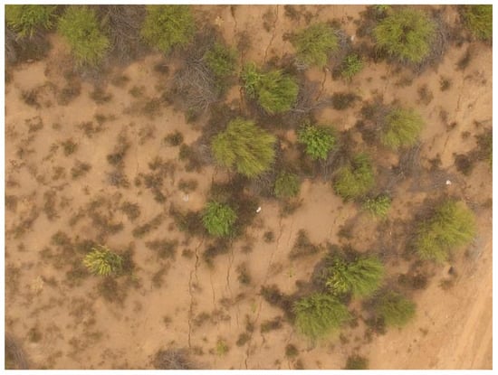
Figure 1.
The UAV image synthesized through the RGB band.

Table 1.
UAV image data parameter information.
2.1.2. Research Methods
This article proposes a surface crack extraction method based on machine learning of UAV images and the quantitative feature information acquisition method. A flowchart is shown in Figure 2. First, cracks are extracted from UAV images based on machine learning, then the crack extraction image is preprocess, and finally the feature information from the cracks is obtained. Specific descriptions of the method are described in subsequent sections.
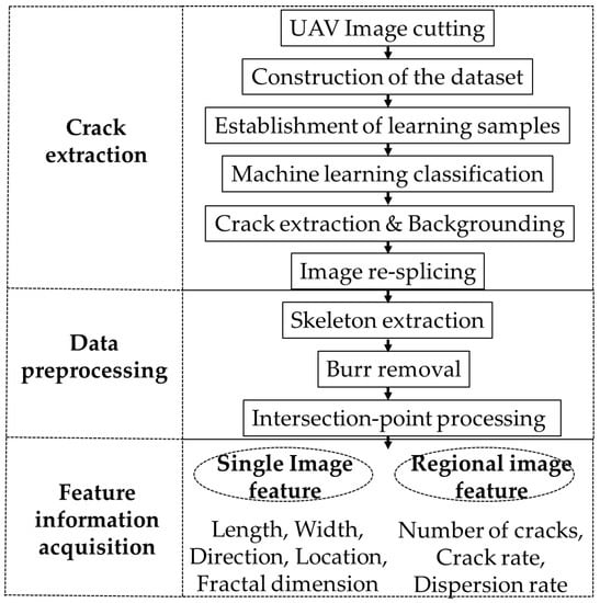
Figure 2.
Flowchart of the crack extraction and feature information acquisition methods for a UAV image.
2.2. Crack Extraction Method Based on Machine Learning
2.2.1. Dataset Construction and Crack Extraction Steps
Crack extraction using UAV images is a high-resolution, flexible-maneuverability, high-efficiency, and low-operating-cost method. However, the existing crack extraction methods based on UAV images inevitably have some erroneous pixels because of the complexity of background information. Though image cutting to reduce the complexity of the background information of an UAV image and then extracting crack image and re-splicing proved to be a reliable method of crack extraction [9], after image cutting, the number of images increases. It is reasonable to extract cracks only from the sub-images containing cracks. Therefore, the sub-images are divided into two categories through machine learning: cracks and no cracks; the steps in the method are shown in Figure 2.
First, a UAV image is cut into 50 × 50 pixel sub-images. Second, datasets are constructed based on different background information from the sub-image: bare ground, soil crusts, and green vegetation. Third, with cracks and no cracks as labels and RGB three-band values as features, 400 images are selected for each dataset to establish training samples. Fourth, using the machine learning method of support vector machine (SVM) [18] and the dimensionality reduction method of F-Score feature selection [19], the sub-images in each dataset are divided into two categories, cracks and no cracks, and the leave-one-out cross-validation and permutation test are used for accuracy verification [20]. Fifth, cracks from sub-images with cracks are extracted and sub-images without cracks are backgrounded. Sixth, the processed sub-images are re-spliced to obtain the results of an UAV image crack extraction. Figure 3 shows the classification results and crack extraction results of each dataset.
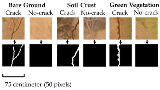
Figure 3.
Classification results of each dataset, crack extraction, and background processing results.
It needs to be specifically explained that, when constructing the datasets of sub-images, 10% is taken as the threshold. When the proportion of soil crusts in a sub-image is greater than 10%, it is classified as a soil crust dataset. When the proportion of green vegetation is greater than 10%, it is classified as a green vegetation dataset. When the soil crusts and green vegetation are both greater than 10%, it is classified as a dataset of higher proportion. The remaining sub-images are classified as bare field datasets.
SVM is a two-class classification model. Its basic model is a linear classifier that searches for separation hyperplanes with a maximal interval in the feature space. V-SVM is chosen as the algorithm model in this study [21]. In the case of linear separability, the V-SVM model is as follows [9]:
where represents a relaxation variable, l represents the amount of variables, w represents the normal vector of the classification hyperplane in the high-dimensional space, b is the constant term, and represents the training set. The parameter v can be used to control the number and error of support vectors. In addition, it is also easier to choose. Parameter represents two types of points (classes −1 and +1) that are separated by an interval of .
2.2.2. Leave-One-Out Cross-Validation and Permutation Test
The accuracy of the crack extraction method was verified by the leave-one-out cross-validation and permutation test.
The leave-one-out cross-validation was used to divide a large dataset into k small datasets. Then, k − 1 was used as the training set and the other was used as the test set. Then, the next one was selected as the test set, and the remaining k − 1 was selected as the training set. By analogy, the k classification accuracy was obtained and the average value was taken as the final classification accuracy of the dataset.
Using the BG dataset (bare ground dataset) as an example, the data from 400 images of this dataset were divided into 200 groups and each group contained one crack image and one no-crack image. We selected 1 group as the test set and the remaining 199 groups as the training set to obtain a classification accuracy. Then, we selected another group as the test set and the remaining 199 groups as the training set, once again obtaining a classification accuracy. By analogy, each of the 200 groups was used as one test set for machine learning and 200 classification accuracy rates were finally obtained. Their average value was taken as the final classification accuracy of the BG dataset.
Statistically significant p-values were obtained by permutation tests. The permutation test is a method proposed by Fisher that is computationally intensive, uses a random arrangement of sample data to perform statistical inference, and is widely used in the field of machine learning. Its specific use is similar to bootstrap methods by sequentially replacing samples, recalculating statistical tests, constructing empirical distributions, and then inferring the p-value based on this. It assumes that N replacement tests are performed, and the classification accuracy rate obtained by n replacement tests is higher than the true accuracy rate; then, p-value = n/N. When the classification accuracy rate obtained without the replacement test is higher than the true accuracy rate, it is usually recorded as p-value <1/N: the smaller the p-value, the more significant the difference. In this article, N = 1000 permutation tests are performed on the three datasets.
2.3. Image Preprocessing Method
The results of UAV image crack extraction cannot be directly used to calculate feature information, such as the crack length, etc. Therefore, before feature calculation, image preprocessing methods such as skeleton extraction and burr removal are also required.
2.3.1. Skeleton Extraction
Skeletonization (also known as thinning) is an image preprocessing technique that is important in many applications such as pattern recognition, data compression, and data storage [22]. The image skeleton can be considered the result of image thinning. At present, there are many thinning algorithms, such as Hilditch thinning algorithm [23], Pavlidis thinning algorithm [24], etc. It is mainly divided into iterative and non-iterative methods. In iterative methods, a refinement algorithm generates a skeleton by checking and deleting contour pixels in the iterative process in a sequential or parallel manner, and it is also divided into parallel iteration and sequential iteration. Among them, Zhang–Suen algorithm is a parallel iterative algorithm [25] and K3M (Khalid, Marek, Mariusz, and Marcin) algorithm is a sequential iterative algorithm [26]. In this article, K3M algorithm is adopted. The idea of this algorithm is to extract the peripheral contour of the target and to then use the contour to corrode the boundary of the target image until it can no longer be corroded. The crack skeleton was extracted by the K3M method, and the result is shown in Figure 4.
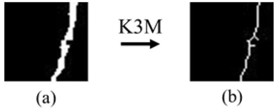
Figure 4.
The results of the crack skeleton extraction by K3M: (a) an image of crack extraction; (b) an image of skeleton extraction.
2.3.2. Burr Removal
The current skeleton extraction algorithm usually cannot obtain the idealized crack skeleton, which will produce burrs [27], as shown in Figure 4b. Therefore, it is necessary to adopt a reasonable method for burr removal. This article proposes a node-based burr removal method.
First, node recognition is performed, as shown in Figure 5, and the skeleton pixel value is 1 and the others are 0. Second, an 8-pixel neighborhood of the skeleton pixel is identified, when the number of skeleton pixels is 1, this skeleton pixel is the endpoint; when the number is 2, this skeleton pixel is the junction point; and when the number is more than 2, this skeleton pixel is an intersection point. Third, branch length identification is performed on all skeleton intersection points to obtain the number of skeleton pixels in each branch. Fourth, setting a threshold, when the number of branch skeleton pixel is less than the threshold, this branch is considered a burr and removed, as shown in Figure 6c1; when there are multiple branches with a skeleton pixel greater than the threshold, the branch is reserved, as shown in Figure 6c2.
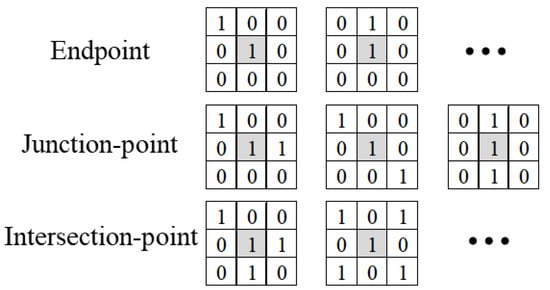
Figure 5.
Node recognition.
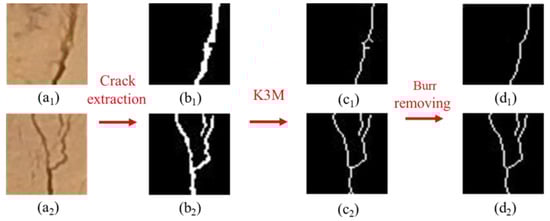
Figure 6.
The results of burr removal from a skeleton image. (a1,a2) are original images, (b1,b2) are images of crack extraction, (c1,c2) are images of skeleton extraction, and (d1,d2) are images of skeleton burr removal.
It should be noted that the threshold is usually close to the crack width. This is because burrs appear in the width direction of the crack, and their length usually does not exceed the crack width.
2.3.3. Intersection-Point Processing
The phenomenon of cracks branching and intersecting is inevitable, and this brings greater difficulties to the acquisition of feature information such as the number, length, width, and direction of surface cracks. Therefore, this article adds the step of intersection-point processing in data preprocessing. The purpose is to break the branching and intersecting cracks such that there are only two node types in the skeleton pixels, as shown in Figure 7: endpoint and junction point. Although this method will cause a small part of the crack to lose a length of 1 pixel, the length of the crack is usually much larger than 1 pixel and, thus, the error is negligible. At the same time, this can greatly reduce the complexity of the calculation method for crack feature information.
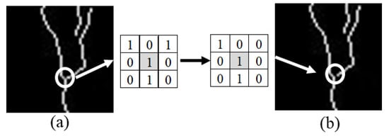
Figure 7.
The result of intersection-point processing on the skeleton image after removing burrs: (a) an image of skeleton burr removal; (b) an image of intersection-point processing.
2.4. Quantitative Acquisition Method of Crack Feature Information
2.4.1. Crack Length
The crack length is calculated using the skeleton image. As shown in Figure 8, the black line segment represents the particle distance of adjacent pixels. For the endpoint pixels, there are two situations in the 8-pixel neighborhood of the skeleton pixel, as shown in Figure 8 , , the particle distances are = 1 pixel and = pixels. For the junction-point pixels, there are three situations in the 8-pixel neighborhood of the skeleton pixel, as shown in Figure 8 , the particle distances are = 2 pixels, = 1 + pixels, and = 2 pixels.
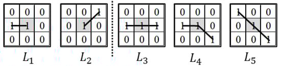
Figure 8.
The particle distance of an 8-pixel neighborhood of the skeleton pixel.
The equation for crack length is
where l is the true length of a single pixel, and represent the number of skeleton pixels and the particle distance in different situations, and the value of t ranges from 1 to 5.
2.4.2. Crack Width
Crack width refers to the number of pixels in the vertical direction of the crack along the strike. Any pixel on the crack skeleton has a width value. Therefore, on the basis of the above method for crack length, the width of each skeleton pixel is calculated separately. The calculation method is shown by the black two-way arrow in Figure 9 below, and finally, the average value is taken as the crack width.
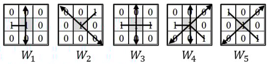
Figure 9.
Statistical direction of crack width.
In particular, when the 8-pixel neighborhood of the skeleton pixel is shown in Figure 10 , the width is half the sum of the two vertical crack pixels as the pixel value of the skeleton pixel. In other cases, the width direction is the vertical or angled direction of the particle distance.
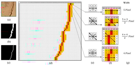
Figure 10.
Statistical direction and calculation method for crack width (red pixels are skeleton pixels, and yellow pixels are crack pixels): (a) the original crack image, (b) the crack extraction image, (c) the skeleton extraction image, (d) the table form of the crack extraction and skeleton extraction results, (e) the result of node recognition and width statistical direction of each skeleton pixel, (f) the calculation method for crack width, and (g) the resulting crack width.
Example: as shown in Figure 10, it can be seen that the width of the first pixel point of this crack is 5 pixels, that of the second is 4 pixels, that of the third is 4 pixels, etc. The calculation result of the average crack width is 3.36 pixels.
2.4.3. Crack Direction
This article proposes a method for calculating the crack direction based on the regression equation, taking true north as the y-axis, true east as the x-axis, and any one point as the origin to establish a rectangular coordinate system. The skeleton extraction diagram in Figure 10c is converted into the rectangular coordinate diagram shown in Figure 11, and the regression equation is calculated using Equations (4)–(6) with y = 3.9053x − 119.46. The crack direction α is calculated using Equation (7), and its value is 14.4°.
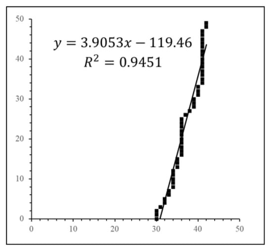
Figure 11.
The result of converting the skeleton pixels to the rectangular coordinate diagram.
2.4.4. Crack Location
The crack location is of great significance for land reclamation. In this article, the center point of the crack skeleton is used as the parameter crack location. As shown in Figure 12, the middle point A of the image represents the shooting position of the UAV and its latitude and longitude are and , respectively, which can be obtained through the image parameters. The middle point of crack B represents the center point of the crack skeleton. The number of pixels between middle point A and middle point B of the image along the longitude and latitude directions is ±m and ±n (± represents the direction; when B is located to the east or north of point A, use +, and when B is located to the west or south of point A, take −), the ground sampling distance (GSD) is l; p and q are the true distances represented by 1° of longitude and latitude, respectively; and then, the longitude and latitude are calculated from the middle of crack B:
Figure 12.
The crack location in a UAV image.
2.4.5. Crack Fractal Dimension
Fractal dimension can be used as a measure of image texture roughness, and it is widely used in the extraction of cracks [28]. The fractal dimension of the linear features of surface cracks and similar linear features in the image are accurately calculated and can better extract the feature information of surface cracks. Commonly used fractal dimensions include Hausdorff dimension, Box Counting dimension (box dimension), Minkowski–Bouligand dimension, etc. [29]. This article uses the box dimension to calculate the fractal dimension of the crack. Its definition is shown in the following Equation (9). The graph is divided into small boxes, where r is the value of the side length of the box in the side length of the graph, and is the number of boxes occupied by the crack. We calculate for different r and apply the least square to fit the array (, ), as shown in Equations (10)–(12), where the fractal dimension D = β.
2.4.6. The Number of Cracks
Based on MATLAB’s bwlabel function, the number of connected components is n. Then, based on the node recognition results, the number of intersection points is m. Therefore, the number of cracks is the sum of m and n. As shown in Figure 13, the statistics show that the connected components n is 2, the intersection point m is 1, and the number of cracks is 3.
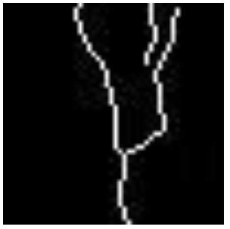
Figure 13.
A skeleton extraction image of intersecting crack.
2.4.7. Crack Rate and Dispersion Rate
In order to comprehensively reflect the distribution characteristics of cracks, the crack rate is usually used as the crack measurement and analysis index. The crack rate is the percentage of the crack area to the study area. However, this method cannot adequately reflect the distribution of a crack. As shown in Figure 14, with two distributions of multiple cracks in Figure 14a,b, the crack rates are calculated as the same, but it can be seen from the figure that there are obvious differences in the distribution of cracks in the two situations; therefore, only the crack rate cannot reflect the true distribution of regional cracks.
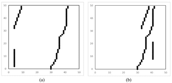
Figure 14.
Two distributions of multiple cracks. (a) shows the scattered distribution of three cracks, (b) shows the concentrated distribution of three cracks.
In view of this, this article proposes a method for calculating the dispersion rate, which reflects the distribution of cracks in the study area through a combination of the crack rate and the dispersion rate. The crack rate shows the size of the crack area, which is also called the areal density of the crack. Its calculation method is the ratio of the crack area to the image area, as shown in Equation (13). The dispersion rate shows the dispersion of cracks, reflecting that the distribution of the cracks is relatively concentrated or scattered. The calculation method is as follows:
The first step is to obtain the center point (, ) of all the crack pixels. The second step is to calculate the average Euclidean distance D/S between all the crack pixel points and the crack center point. The third step is to perform normalization. Theoretically, the maximum average Euclidean distance will not exceed half of the diagonal length of the image. Therefore, the ratio of the average Euclidean distance to half of the diagonal length of the image is used as the normalized dispersion rate. As shown in Equations (14)–(18), the essence of the dispersion rate is the average Euclidean distance between all crack pixels and the center point normalized: the lower the value, the closer all the skeleton points are to the center point and the more concentrated the distribution, and the higher the value, the farther all the crack points are from the center point and the more scattered the distribution.
where a and b represent the length and width of the image, respectively; i represents the crack number; j represents the pixel of each crack; and represent the coordinates of any crack pixel in the plane rectangular coordinate system; m represents the number of cracks; represents the number of crack pixels of the ith crack; and represent the coordinates of the crack center point in the rectangular coordinate system; S represents the number of all crack pixels; D represents the sum of the Euclidean distance of all crack pixels and the crack center; represents the area of the ith crack; σ represents the normalized dispersion rate; and δ represents the crack rate. The range of the two values is between 0 and 1.
Figure 14a,b have the same crack rate δ. By calculating the dispersion rate = 0.3016 > = 0.1874, the distribution of cracks in Figure 14a is more dispersed than that in Figure 14b, which is consistent with what the image shows. It is proven that this method can be used to reflect the dispersion degree of the cracks.
3. Results and Discussion
3.1. Results of Crack Extraction
This article proposes a method for crack extraction of UAV images based on machine learning. The machine learning method uses SVM, and the dimensionality reduction method uses F-score. The parameter selection of the F-score is 0.1:0.1:1, which means that, according to the weight/F value, the first 0.1 features are selected first, then 0.1 is used as the step size, and the features are selected gradually to 1 (100%). The verification method uses leave-one-out cross-validation and the permutation test. The number of permutation tests is 1000.
The results are shown in Figure 15 and Table 2. We can find that, for the three datasets, when full feature selection is used for the image, the classification accuracy and AUC value are the largest, and the p-value is less than 0.001, which proves that machine learning can effectively classify whether there are cracks in the UAV sub-images. Among them, the classification accuracy of the bare land dataset reached 87.75%, the classification accuracy of the soil crust dataset reached 87.25%, and the classification accuracy of the green vegetation dataset reached 93.50%. The overall accuracy rate reached 89.5%.
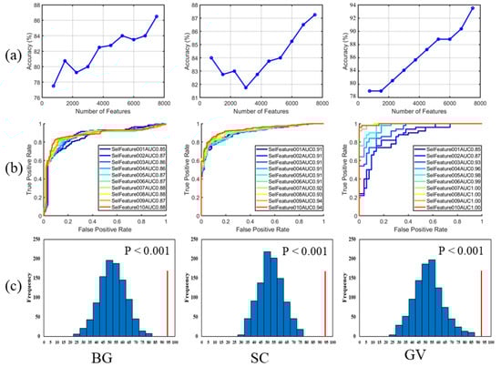
Figure 15.
The results of leave-one-out cross-validation and the permutation test. BG is the bare ground dataset, SC is the soil crust dataset, and GV is the green vegetation dataset. (a) is the accuracy change result for different dimension selection, (b) is the result of ROC curve and its AUC value, (c) is the result of the permutation test.
Table 2.
Final classification results.
Through the above method, the UAV sub-images are divided into two categories: cracks and no cracks. For crack images, the crack extraction method of threshold segmentation is used. For no crack images, the black background method is used. Finally, each processed image is stitched together, and the final UAV image crack extraction effect is shown in Figure 16b.
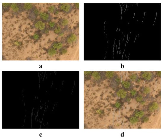
Figure 16.
Image preprocessing results: (a) a UAV image synthesized through the RGB band, (b) the result of crack extraction, (c) a skeleton image after data preprocessing, and (d) the comparison of the final schematic diagram of the crack extraction effect in the UAV image and original UAV image.
3.2. Image Preprocessing Results
The crack extraction image obtained above is performed by skeleton extraction, burr removal, and intersection-point processing, as shown in Figure 16c, which provides data support for subsequent quantitative acquisition of crack feature information.
3.3. Quantitative Calculation Results of Crack Feature Information
3.3.1. Single Crack Feature Calculation Results and Accuracy Verification
The single crack features include crack length, average width, direction, location, and fractal dimension. The statistics for crack length and direction use the skeleton image after data preprocessing. The crack width, location, and fractal dimension use the crack extraction image.
The true value measurement method for the crack feature information is as follows: the true value of the crack length is measured by the traverse method. The true value of the crack width is obtained by measuring the width of five different parts of the crack and by taking the average value. The true value of the crack direction is determined by the compass. The true value of location is measured by a handheld GPS (Global Positioning System). In this study area, five cracks at different locations were randomly selected for accuracy verification by comparing the true value and the image value calculated. As shown in Figure 17.
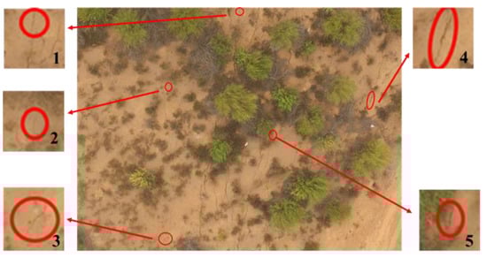
Figure 17.
Five cracks at different locations were randomly selected for accuracy verification in this study area.
The results of the image calculation values and field measurement values are shown in Table 3. We can find that all the crack length errors are less than 10%, that the crack width errors are less than 19%, that the direction difference is less than 3°, and that the location distance difference is less than 3 m. This shows that the results calculated by the method in this article are relatively close to the true value, which is an effective method for crack feature information calculation.
Table 3.
The comparison result of crack feature extraction and true value measurement.
3.3.2. Regional Crack Feature Calculation Results
Regional crack feature refers to the characteristics reflected by all cracks in the study area, including the number of cracks, crack rate, and dispersion rate. The statistics for the number of cracks use the skeleton image after data preprocessing. The crack rate and dispersion rate use the crack extraction image. The results are shown in Table 4.
Table 4.
The results of regional crack feature calculation.
All of the cracks in the study area were calculated. The statistical results for crack length and crack width are shown in Figure 18. We can see that the crack length is mainly within 5 m, accounting for 96.74%, and that the crack average width is mainly within 0.04 m, accounting for 95.65%. The statistical results of the crack direction are shown in Figure 19. The number of cracks is counted at 15° intervals. We can see that the crack direction is generally in the north–south direction. The statistical results of the crack fractal dimension are shown in Figure 20, from which we can see that the crack fractal dimension is between 1.0750 and 1.3521. The surface cracks show an excellent linear correlation, which shows that the regional surface cracks in this image have good statistical self-similarity. It has a good fractal geometry structure. The calculated result of box dimension shows that coal mining surface cracks have fractal dimensions. To a certain extent, surface cracks do not exist in isolation and have systems with similar or identical features inside. This conclusion is consistent with Mao Cuilei’s conclusion in the study of the distribution characteristics of surface cracks, and his result showed that the fractal box dimension of surface cracks in the region is between 1.08–1.35 [30].
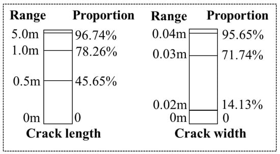
Figure 18.
The statistical results for crack length and crack width.
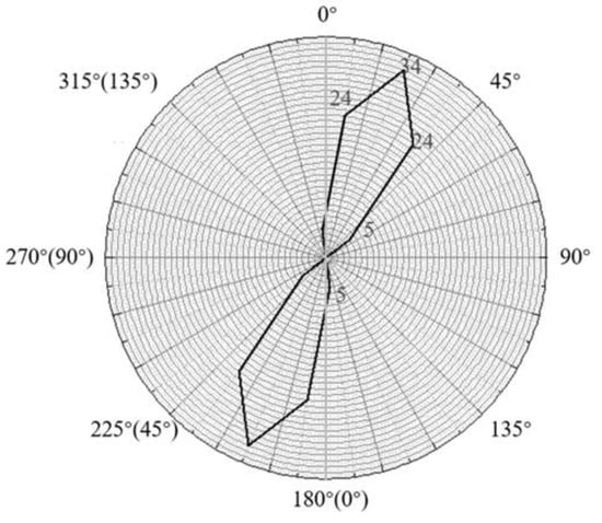
Figure 19.
The statistical result for all crack directions.
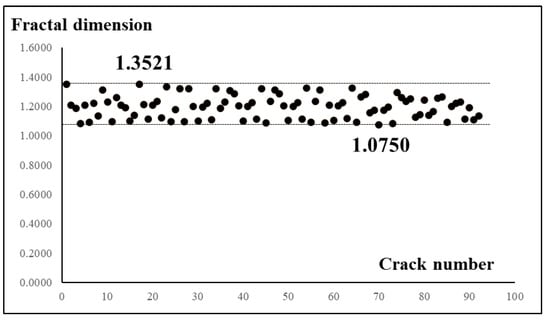
Figure 20.
The statistical result for all crack fractal dimensions.
4. Conclusions
This article proposes a surface crack extraction method based on machine learning of the UAV image, the data preprocessing steps, the content of the crack feature information, and the calculation method. The reliability of the method is proven by accuracy verification, and the following conclusions are obtained:
- The error in surface crack extraction from a UAV image mainly comes from complex background information such as vegetation and soil crust. Using machine learning to classify the sub-images, then to extract cracks, and to re-splice is an effective method to avoid the error. The total accuracy reached 89.50%.
- By acquiring the single crack feature information content—crack length, width, direction, fractal dimension, and location—it can clearly describe the feature information of any crack. In this study area, the crack length is mainly within 5 m, the crack average width is mainly within 0.04 m, the crack direction is generally in the north–south direction, and the crack fractal dimension is between 1.0750 and 1.3521.
- The concept and calculation method for the dispersion rate are introduced. The crack rate is used to show the size of the crack area, and the dispersion rate is used to show the concentration or dispersion of the cracks in the area. This method more clearly and completely describes the distribution characteristics of regional cracks.
Cracks are a common geological disaster. The scientific repair of cracks requires us to reasonably classify and evaluate different degrees of cracks. This article not only achieves higher-precision crack extraction but also obtains a reliable quantitative calculation method for crack feature information, which can provide data support for further research on the development and risk evaluation of surface cracks. Furthermore, we will use the crack feature information as the evaluation index and the value obtained by quantitative calculation as the evaluation basis to evaluate the damage degree of the crack and then propose a reasonable repair plan.
Author Contributions
Conceptualization, F.Z. and Z.H.; methodology, F.Z. and Y.F.; software, F.Z.; formal analysis, K.Y.; investigation, Y.F.; resources, K.Y.; data curation, F.Z.; writing—original draft preparation, F.Z.; writing—review and editing, Z.H.; project administration, Z.F.; funding acquisition, M.B. All authors have read and agreed to the published version of the manuscript.
Funding
This research was funded by the Research and Demonstration of Key Technology for Water Resources Protection and Utilization and Ecological Reconstruction in Coal Mining areas of Northern Shaanxi; the grant number is 2018SMHKJ-A-J-03.
Data Availability Statement
The data presented in this study are openly available.
Acknowledgments
Thanks to the Institute of Land Reclamation and Ecological Reconstruction and Shaanxi Coal Group for their help in this research.
Conflicts of Interest
The authors declare no conflict of interest.
References
- Xu, L.; Li, S.; Cao, X.; Somerville, I.D.; Cao, H. Holocene intracontinental deformation of the northern north china plain: Evidence of tectonic ground fissures. J. Asian Earth Sci. 2016, 119, 49–64. [Google Scholar] [CrossRef]
- Wang, W.; Yang, Z.; Kong, J.; Cheng, N.; Duan, L.; Wang, Z. Ecological impacts induced by groundwater and their thresholds in the arid areas in northwest china. Environ. Eng. Manag. J. 2013, 12, 1497–1507. [Google Scholar] [CrossRef]
- Youssef, A.M.; Sabtan, A.A.; Maerz, N.H.; Zabramawi, Y.A. Earth fissures in Wadi Najran, kingdom of Saudi Arabia. Nat. Hazards 2014, 71, 2013–2027. [Google Scholar] [CrossRef]
- Chen, Y.-G. Logistic models of fractal dimension growth of urban morphology. Fractals 2018, 26, 1850033. [Google Scholar] [CrossRef]
- Stumpf, A.; Malet, J.P.; Kerle, N.; Niethammer, U.; Rothmund, S. Image-based mapping of surface fissures for the investigation of landslide dynamics. Geomorphology 2013, 186, 12–27. [Google Scholar] [CrossRef]
- Ludeno, G.; Cavalagli, N.; Ubertini, F.; Soldovieri, F.; Catapano, I. On the combined use of ground penetrating radar and crack meter sensors for structural monitoring: Application to the historical consoli palace in gubbio, italy. Surv. Geophys. 2020, 41, 647–667. [Google Scholar] [CrossRef]
- Sharma, P.; Kumar, B.; Singh, D. Novel adaptive buried nonmetallic pipe crack detection algorithm for ground penetrating radar. Prog. Electromagn. Res. M 2018, 65, 79–90. [Google Scholar] [CrossRef][Green Version]
- Shruthi, R.B.V.; Kerle, N.; Jetten, V. Object-based gully feature extraction using high spatial resolution imagery. Geomorphology 2011, 134, 260–268. [Google Scholar] [CrossRef]
- Zhang, F.; Hu, Z.; Fu, Y.; Yang, K.; Wu, Q.; Feng, Z. A New Identification Method for Surface Fissures from UAV Images Based on Machine Learning in Coal Mining Areas. Remote. Sens. 2020, 12, 1571. [Google Scholar] [CrossRef]
- Peng, J.; Qiao, J.; Leng, Y.; Wang, F.; Xue, S. Distribution and mechanism of the ground fissures in wei river basin, the origin of the silk road. Environ. Earth Sci. 2016, 75, 718. [Google Scholar] [CrossRef]
- Zheng, X.; Xiao, C. Typical applications of airborne lidar technolagy in geological investigation. Int. Arch. Photogramm. Remote Sens. Spat. Inf. Sci. 2018, 42, 3. [Google Scholar] [CrossRef]
- Nex, F.; Remondino, F. Uav for 3d mapping applications: A review. Appl. Geomat. 2014, 6, 1–15. [Google Scholar] [CrossRef]
- Dhivya, R.; Prakash, R. Edge detection of satellite image using fuzzy logic. Clust. Comput. 2019, 22, 11891–11898. [Google Scholar] [CrossRef]
- Papari, G.; Petkov, N. Edge and line oriented contour detection: State of the art. Image Vis. Comput. 2011, 29, 79–103. [Google Scholar] [CrossRef]
- Verschuuren, M.; De Vylder, J.; Catrysse, H.; Robijns, J.; Philips, W.; De Vos, W.H. Accurate detection of dysmorphic nuclei using dynamic programming and supervised classification. PLoS ONE 2017, 12, e0170688. [Google Scholar] [CrossRef] [PubMed]
- Fujita, Y.; Shimada, K.; Ichihara, M.; Hamamoto, Y. A method based on machine learning using hand-crafted features for crack detection from asphalt pavement surface images. In Proceedings of the Thirteenth International Conference on Quality Control by Artificial Vision 2017, Tokyo, Japan, 14 May 2017; International Society for Optics and Photonics: Bellingham, WA, USA, 2017; Volume 10338, p. 103380I. [Google Scholar] [CrossRef]
- Hoang, N.-D.; Nguyen, Q.-L. A novel method for asphalt pavement fissure classification based on image processing and machine learning. Eng. Comput. 2019, 35, 487–498. [Google Scholar] [CrossRef]
- Wang, Y.; Zhu, X.; Wu, B. Automatic detection of individual oil palm trees from uav images using hog features and an svm classifier. Int. J. Remote Sens. 2019, 40, 7356–7370. [Google Scholar] [CrossRef]
- Tao, P.; Yi, H.; Wei, C.; Ge, L.Y.; Xu, L. A method based on weighted F-score and SVM for feature selection. In Proceedings of the 2013 25th Control and Decision Conference (CCDC), Guiyang, China, 25–27 May 2013. [Google Scholar] [CrossRef]
- Peng, Y.; Zhang, X.; Li, Y.; Su, Q.; Liang, M. Mvpani: A toolkit with friendly graphical user interface for multivariate pattern analysis of neuroimaging data. Front. Neurosci. 2020, 14, 545. [Google Scholar] [CrossRef]
- Wang, X.; Wu, S.; Li, Q.; Wang, X. v-SVM for transient stability assessment in power systems. In Proceedings of the Autonomous Decentralized Systems. In Proceedings of the ISADS 2005, Chengdu, China, 4–8 April 2005. [Google Scholar] [CrossRef]
- Zhou, C.; Yang, G.; Liang, D.; Yang, X.; Xu, B. An integrated skeleton extraction and pruning method for spatial recognition of maize seedlings in mgv and uav remote images. IEEE Trans. Neurosci. Remote Sens. 2018, 56, 4618–4632. [Google Scholar] [CrossRef]
- Naseri, M.; Heidari, S.; Gheibi, R.; Gong, L.H.; Sadri, A. A novel quantum binary images thinning algorithm: A quantum version of the hilditch’s algorithm. Opt. Int. J. Light Electron Opt. 2016, 131, 678–686. [Google Scholar] [CrossRef]
- Abu-Ain, W.; Abdullah, S.N.H.S.; Bataineh, B.; Abu-Ain, T.; Omar, K. Skeletonization algorithm for binary images. Procedia Technol. 2013, 11, 704–709. [Google Scholar] [CrossRef]
- Patel, R.B.; Hiran, D.; Patel, J.M. Fingerprint image thinning by applying zhang suen algorithm on enhanced fingerprint image. Int. J. Comput. Sci. Eng. 2019, 7, 1209–1214. [Google Scholar] [CrossRef]
- Saeed, K.; Tabędzki, M.; Rybnik, M.; Adamski, M. K3m: A universal algorithm for image skeletonization and a review of thinning techniques. Int. J. Appl. Math. Comput. Sci. 2010, 20, 317–335. [Google Scholar] [CrossRef]
- Qin, X.; Cai, C.; Zhou, C. An algorithm for removing burr of skeleton. J. Huazhong Univ. Sci. Technol. (Nat. Sci. Ed.) 2004, 12, 28–31. [Google Scholar] [CrossRef]
- Zhao, H.; Yang, G.; Xu, Z. Comparison of Calculation Methods-Based Image Fractal Dimension. Comput. Syst. Appl. 2011, 20, 238–241. [Google Scholar] [CrossRef]
- Chen, C.; Hu, Z. Research advances in formation mechanism of ground fissure due to coal mining subsidence in China. J. China Coal Soc. 2018, 43, 810–823. [Google Scholar] [CrossRef]
- Mao, C. Study on Fracture Distribution Characteristics of Coal Mining Collapse in Loess Hilly Area; China University of Geosciences: Beijing, China, 2018. [Google Scholar]
Publisher’s Note: MDPI stays neutral with regard to jurisdictional claims in published maps and institutional affiliations. |
© 2021 by the authors. Licensee MDPI, Basel, Switzerland. This article is an open access article distributed under the terms and conditions of the Creative Commons Attribution (CC BY) license (https://creativecommons.org/licenses/by/4.0/).