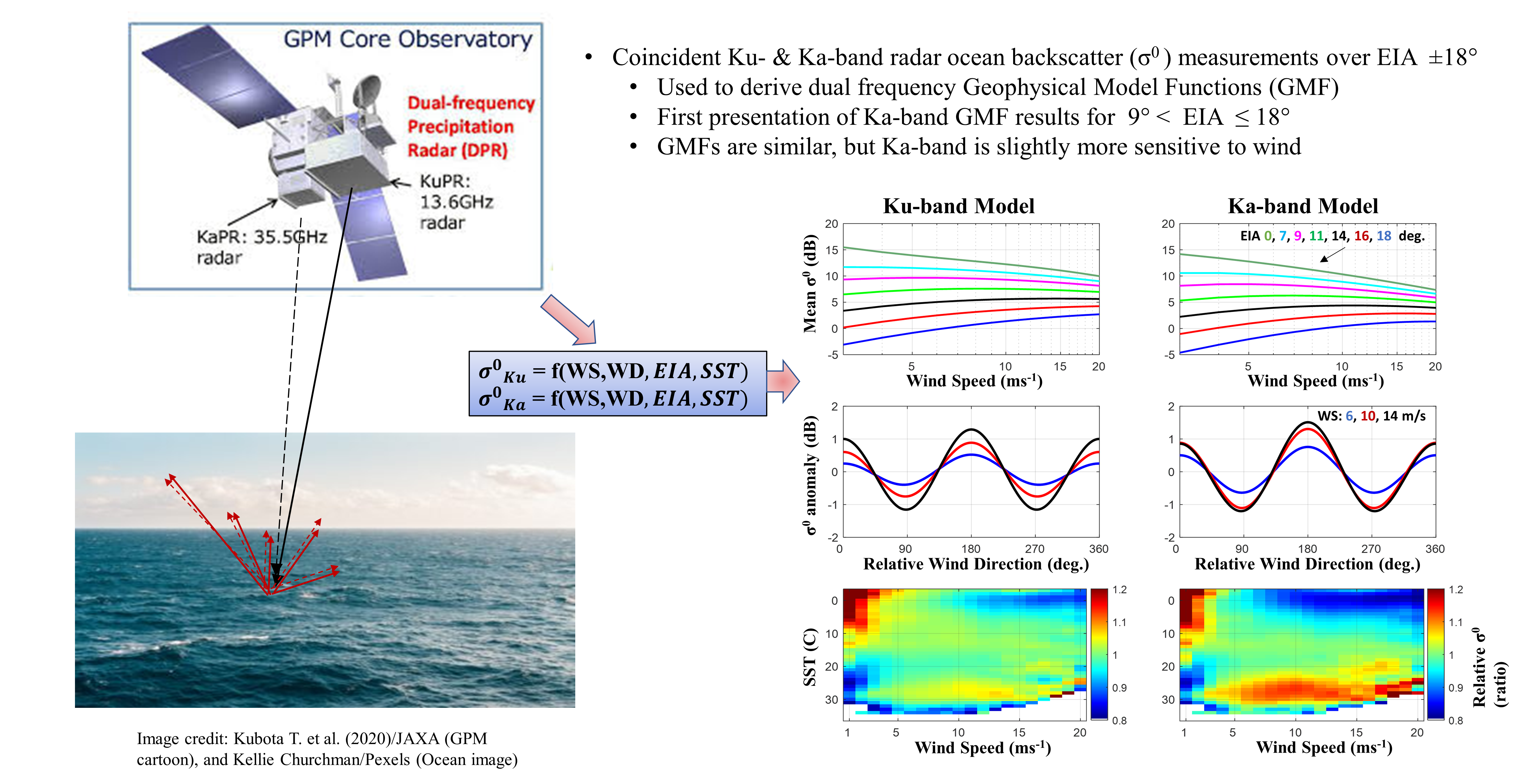
The microwave ocean surface radar backscatter (σ
0) at the GPM DPR incidence angle range (0° to 18°) are dominated by quasi-specular scattering process, but towards the outer swath, the resonant (Bragg) scattering process also becomes significant [
5]. For both regimes, the σ
0 is directly related to the ocean surface wind vector (OVW), SST, and integral wave parameters [
9,
10,
11,
12,
15,
23,
24]. The backscatter can be empirically modeled as a 2nd order Fourier series (higher order terms are negligible),
where
is the sea surface normalized radar cross section at a frequency (
f) and polarization (
p) in dB unit. The model coefficients
,
,
and
are wind speed, EIA and sea-state dependent, and
χ denotes the wind direction relative to the radar azimuth look defined as
χ =
−
, where
is the meteorological wind direction (i.e., the direction where the wind is coming from), and
for DPR, is cross-track azimuth look (flight direction
), both referring to the North. Accordingly,
χ = 0 denotes the upwind specifying that the wind is blowing toward the radar look direction. Since both, Ku and Ka PR onboard GPM operate at only horizontal polarization, all references to polarization are omitted in this paper.
Historically, the radar ocean backscatter GMF has been modeled as a cosine Fourier series [
25,
26], but our initial analysis used both sine and cosine terms in Equation (1). However, after a comprehensive investigation, it was concluded that the sine terms were not statistically significant, and as a result, they were neglected.
Figure 3 illustrates a typical comparison of the GMF, with and without the sine terms, for an EIA = 16
and WS of 16 m/s. The circle symbols are the residual [
] of empirical bin average
, and the red solid line is the full model (Equation (1), sines and cosines) and the blue solid line is the cosine alone GMF. As shown, the contribution of the odd terms is negligible and the
azimuth anisotropy can be well approximated by only even terms.
It should be noted that Equation (2) is the same expression used to model the ocean backscatter at moderate EIAs (20°–70°), but here, as will be depicted in the next section, the term is negative for EIA < 20°, which results in a reversal of upwind and downwind asymmetry, i.e., higher downwind backscatter than the upwind backscatter.
In this section, the dependence and sensitivity of Ku and Ka band σ
0 on EIA, and the ocean surface wind speed, and wind direction are analyzed. Fourier coefficients
and
are derived using σ
0 measurements for each angular beam (EIA) positions, and finally, these coefficients are modeled as a function of wind speed using polynomial fit of appropriate orders. Additionally, the SST dependence of Ku and Ka band σ
0 is discussed. Results of sea state dependence of σ
0 are not included in this paper; however, readers are encouraged to see [
9,
10,
12,
15] for this.
3.1. Isotropic Ku and Ka-Band Model Function at Low Incidence Angles
The
A0 coefficient in Equation (1) is the azimuth independent (isotropic) σ
0 measurement that is directly related to the wind speed (WS) for a particular earth incidence angle (EIA). Thus, it can be modeled as,
In order to analyze,
, the normalized radar backscatter (σ
0) measurements of the Ku and Ka-bands were sorted in
ms
−1 wind speed bins for each of 49 EIA beams. A conservative 3σ filter was applied to each bin to remove outliers (the 3σ values were calculated in linear, not dB, units), and any bin with less than 500 boxes was not included in the analysis. Next, using polynomial regression (in dB space), the bin average σ
0 for each of this EIA position were expanded as a third-order polynomial of log (WS). The use of log (WS) for
reduces the order of the polynomial fit.
where x =
and the numerical values of these coefficients (in dB) are given in the
Table A1 in
Appendix A for EIA 0
to 18.1
(Beams 1 to 25).
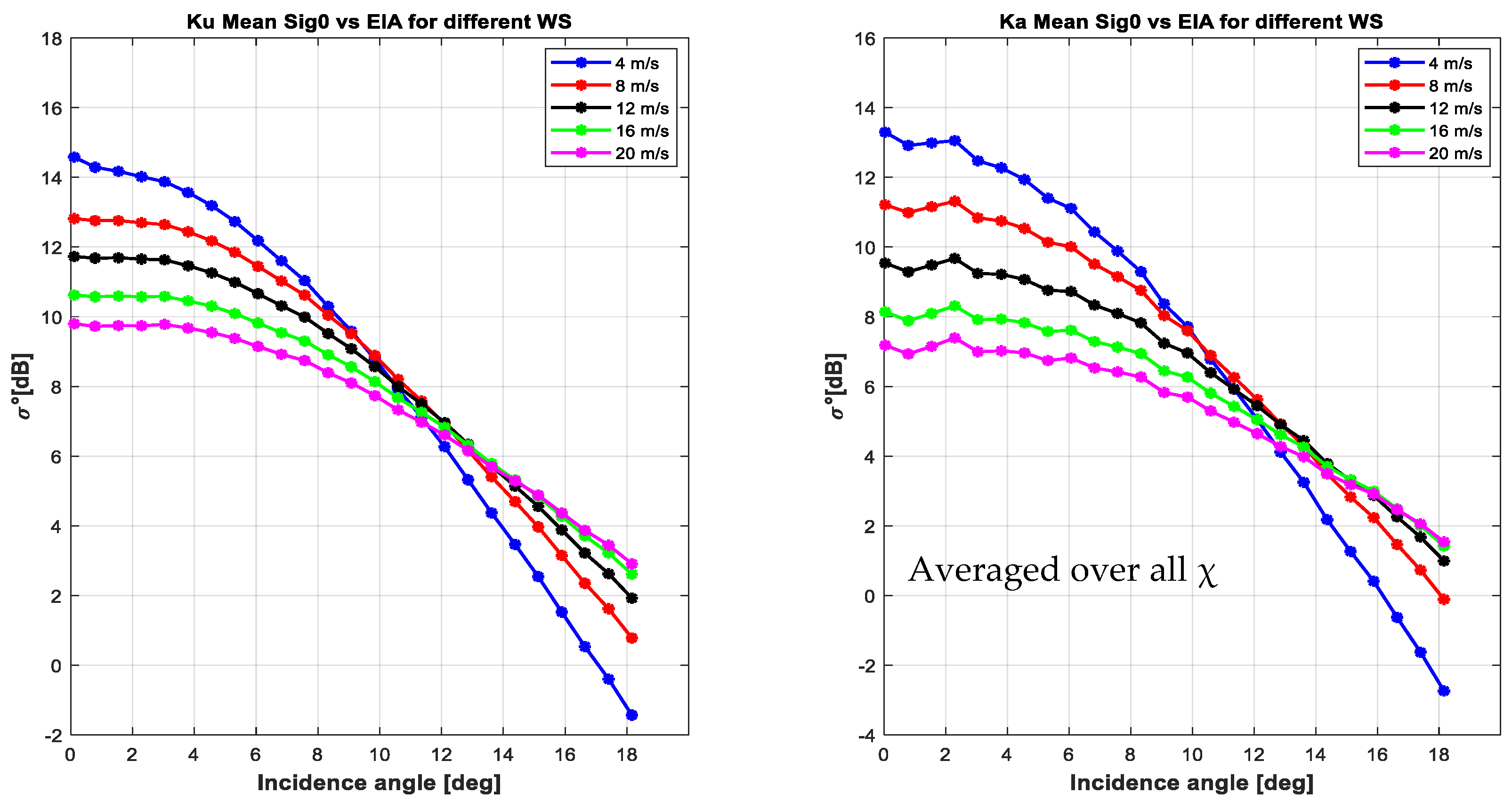
The dependence of
on WS is illustrated in
Figure 4 using a log-log plot, for eight PR beam positions that include EIAs nadir to 18.1
. The circle symbols represent the mean value of σ
0 measurements over all wind directions and the solid lines are their third-order polynomial fits, both in dB. At the higher EIA beam positions, σ
0 monotonically increases with wind speed, whereas it monotonically decreases for lower EIAs near nadir. For the middle EIA beam positions, the σ
0 dependence is not monotonic because there are two different scattering mechanisms involved. Namely, the near nadir backscatter is dominated by quasi-specular scattering that decreases σ
0 with increased ocean roughness, but as EIA increases, Bragg scattering gradually becomes significant that increases σ
0 with WS. These Ku results are consistent with [
5,
6,
7,
8,
9,
10,
11,
12,
15], except for a small calibration bias between TRMM PR and GPM KuPR.
While these results (
Figure 4) are qualitatively similar for Ka PR, there are small differences between the
A0 GMFs (Equation (4)) for Ku and Ka bands, and these differences are also a function of wind speed and incidence angle, as shown in
Figure 5, which plots the differences of mean backscatter values (Δ
A0) of Ku and Ka models as a function of WS for different EIA beam positions. For the lower EIA beams, the difference increases monotonically with WS, but for the higher EIA beams, the difference first decreases with WS for lower to moderate WS, then it increases with WS for higher WS. However, for higher EIA beam positions, the differences are smaller than at lower EIA beam positions, for instance, the difference is less than 1.5 dB at EIA ~ 16
for any WS between 3 and 20 m/s. Beside this, the WS sensitivity or σ
0 gradient, defined as (
), is shown in
Figure 6 as a function of WS for the same beam positions corresponding to
Figure 4. The slope of increase or decrease declines with WS at both bands. For Ka band, it declines slightly more rapidly than at Ku band for low WS region, whereas for medium to higher WS, the slopes are a little higher at Ku band.
Figure 7 shows the scatter diagram of Ku and Ka PR mean σ
0 for six fixed EIA beam positions. Symbols represent the mean σ
0 for different wind speed bins (1 to 20 m/s at
1 m/s steps). As shown, for the outer beam positions (higher EIA), Ku and Ka PR mean σ
0 are linearly correlated, except for higher WS, where σ
0 become flat and start to decrease with WS. The drop of σ
0 with increasing WS begins at relatively lower WS at the inner beam positions (lower EIA) as shown at the bottom panel of the same Figure. These correlations between Ku and Ka PR mean σ
0 could be a useful alternative way to determine one from another, especially for outer beam positions. For example, the missing Ka outer swath for the initial phase of GPM mission (up to 22 May 2018) could be estimated from corresponding Ku band measurements. For higher WS at lower EIA, this approach would be difficult and more prone to error. However, the model derived in this paper (Equation (4)) is reliably applicable for WS 3–20 m/s for all EIA beam positions. Another important implication of
Figure 7 is the variation of dynamic range of wind-roughened σ
0 with EIA. This is shown in
Figure 8, which compares the maximum wind-dependent variation of Ku band mean σ
0 with that at Ka band. As shown, although both have similar dynamic ranges for EIA ~> 9
, Ka band mean σ
0 has higher dynamic range for EIA < 9
.
Finally, the mean values of binned average σ
0 for Ku and Ka bands are shown in
Figure 9 as a function of EIA for different wind speeds. The σ
0 monotonically decreases with increasing incidence angle from nadir to 18.2°. Additionally, the σ
0 decreases monotonically with wind speed at EIAs near nadir, but σ
0 increases monotonically with wind speed near EIA 18.2°, with a transition in the middle where σ
0 becomes relatively insensitive to WS (for WS
ms
−1). For KuPR, this transition occurs over EIA 11°–13
, whereas for KaPR it occurs over EIA 12°–14°. Additionally, these transition regions vary with the relative azimuth look, for upwind/downwind/crosswind directions, as shown for KuPR in
Figure 10 (these variations are proportionately similar at Ka-band which is not shown here). This EIA range of reduced σ
0 variability is useful for the radar inter-calibration between these kinds of instruments [
5]. Therefore, based upon these results, we conclude that the two GMF’s are similar and are applicable for a WS range of 3–20 ms
−1 and for all EIA beam positions.
3.2. σ0 Azimuthal Anisotropy
The directional anisotropy of ocean surface σ
0 is a function of WS, relative wind direction, and EIA. We can separate the directional signal of σ
0 (in dB) by computing the residual of σ
0 as follows,
To analyze the directional anisotropy of both KuPR and KaPR, in accordance with Equation (5), the σ
0 measurements in WS bins (±1 m/s) were further sorted into 10
relative wind direction (
χ) bins. Afterwards, the Fourier series approximation of Equation (2) was applied to the bin average of both Ku and Ka PR
(in dB space), to derive
and
coefficients for each WS and EIA bin position. Finally,
and
Fourier coefficients, thus derived, were modeled as a function of WS using third and seventh order polynomial regressions (in dB space), respectively. Unlike the case of
in Equation (4), use of log (WS) for
and
does not reduce the order of the polynomials, thus WS measurements in linear units were used in these cases.
and,
where
, and the values of the polynomial coefficients
through
and
through
(in dB) are given in the
Table A2,
Table A3, and
Table A4 in
Appendix A for EIA 0
to 18.1
(Beams 1 to 25).
The
and
coefficients, for the corresponding EIA beam positions, are shown as a function of WS in
Figure 11 and
Figure 12, respectively. Symbols in both Figures represent the Fourier coefficients found from Equation (2), and the solid lines represent the corresponding polynomial fits (Equations (6) and (7)). For both bands,
is negative, and the magnitude becomes more negative with increasing WS. Additionally, for the same EIA, the magnitude of the Ka band
is slightly more negative, and the doubling of this coefficient is the measure of upwind-down wind asymmetry. For the
coefficient, both bands have similar patterns, which decrease with increasing WS and reach a minimum (at ~6 m/s (Ku) and ~5 m/s (Ka)). Afterwards, the magnitude of
rapidly increases with WS until it approximately saturates at WS ~= 14 m/s for Ku band and WS ~= 12 m/s for Ka band. The
coefficient is a measure of upwind–crosswind asymmetry or total directional anisotropy, and it increases with EIA.
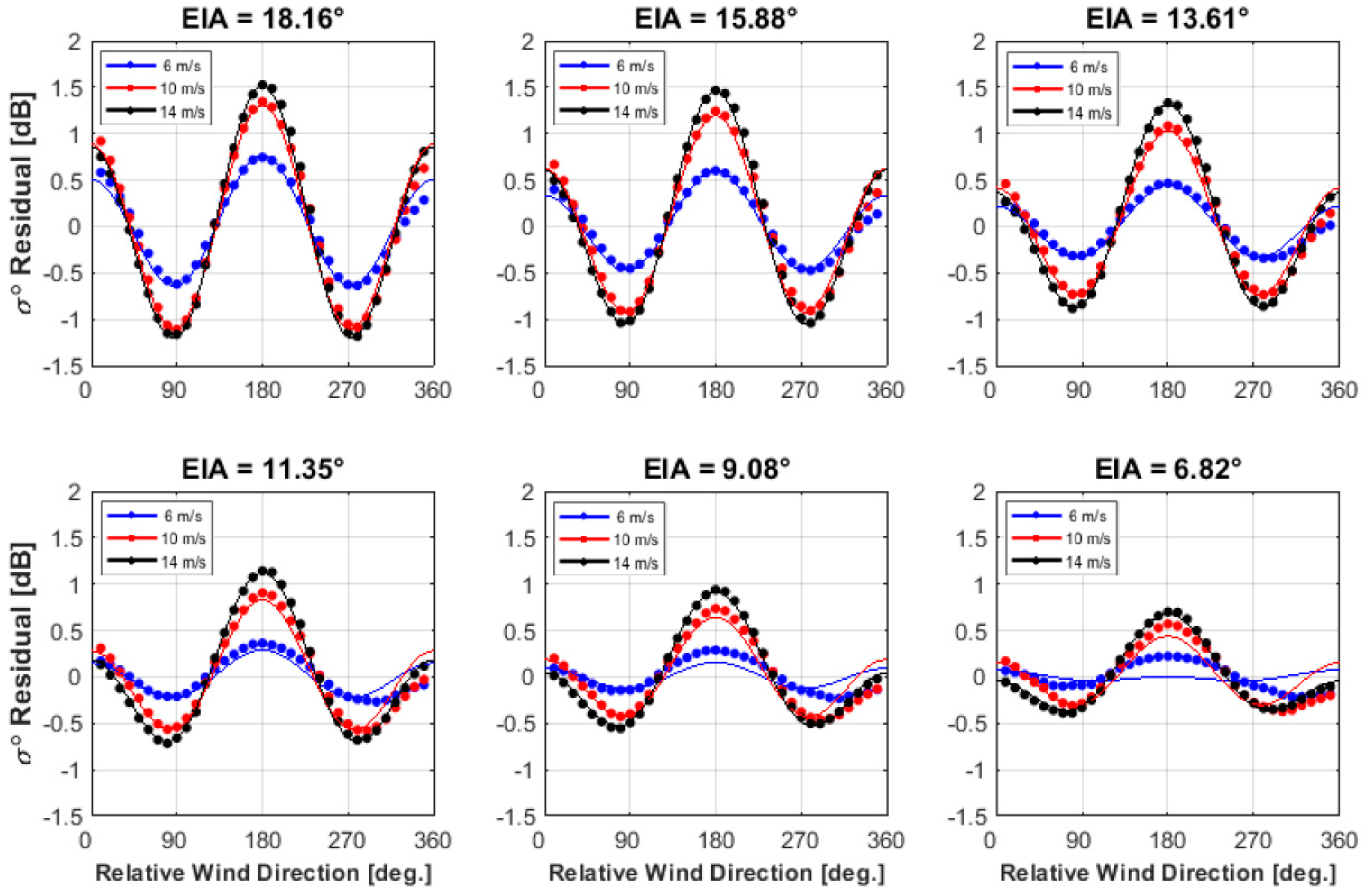
The residual (anomaly) of the KuPR σ
0 is presented in
Figure 13 as a function of relative wind direction for selected EIAs and WS. The symbols are the residual of the measured bin average, and the solid lines are the corresponding model (Equation (5)). As shown, the bi-harmonic directional signal increases with both WS and EIA, and the model is in excellent agreement with the empirical measurements for all cases, except for the 6.8° EIA (and less), which is slightly degraded for relative WD: 270°–360°, especially for lower WS cases. The corresponding results for KaPR are presented in
Figure 14, but for these cases the quality of the model fit is somewhat lacking for the lower three EIAs. For these cases, the model downwind response (relative WD = 180°) is progressively underestimated (at the 0.1 dB level), and the model fit with the empirical measurements for relative WD of 270°–360° disagree at the 0.2 dB level. Since both the Ku and Ka models have issues with this same relative WD range, the empirical measurements are suspect. Further, the model has an even symmetry with relative WD, whereas the empirical measurements have not. The reason for this anomaly is not understood, but given the low EIA, one possible explanation is the effect of ocean wave swell, which has not been considered in this analysis.
The relative difference between the Ku and Ka band σ
0 directional residual (
), is given in
Figure 15 as a function of relative wind direction for the WS averaged over 6–14 m/s at different EIAs. As shown, the maximum difference occurs at the upwind, downwind and crosswind directions which is also a function of the EIA. Now consider the delta-σ
0 residual, calculated at upwind, downwind and crosswind for an EIA ~ 16°, as a function of WS (given in
Figure 16). At the downwind direction, the KaPR has a higher wind direction signal than KuPR for all WS, whereas for the upwind and crosswind, the polarity of the difference depends on WS range.
3.2.1. Upwind and Downwind Asymmetry of σ0
One of the interesting features of the σ
0 WD anisotropy at low EIA is that it has an opposite upwind/downwind asymmetry compared to the conventional scatterometers that operate at moderate incidence angles (20°–70°). As shown in
Figure 13 and
Figure 14, DPR measures a higher σ
0 from the downwind direction than that from the upwind direction, and 2
is the measure of the peak-to-peak upwind/downwind asymmetry. The differences between downwind and upwind σ
0 measurements, separately for both KuPR and KaPR as a function of WS: 3–20 m/s, are shown in
Figure 17 for six different EIAs: 6.8°–18.2°, and it is noted that for all EIAs, the measured σ
0 asymmetry increases with WS of 6–16 m/s. Chu et al. (2012) [
12] also presented similar results for TRMM KuPR and Mouche et al. (2006) [
27] reported the same trends of asymmetries for a C band radar at low incidence angle. However, this paper presents new information concerning a higher upwind/downwind asymmetry for Ka band compared to the Ku band. For example, at EIA ~ 12°, the Ku band asymmetry is about 0.7 dB for a WS of 16 m/s, while it is > 1 dB for Ka band for the same EIA and WS.
3.2.2. Downwind and Crosswind Anisotropy of σ0
For scatterometers operating at moderate EIAs, the
coefficient in Equations (2) and (5), usually defines the peak-to-peak (upwind to crosswind) anisotropy of σ
0. However, for this low EIA range, since
is negative and not negligible, backscatter response at the downwind direction is the sum of
and
. Therefore, the peak-to-peak anisotropy for this EIA range is defined downwind to crosswind which is > 2
.
Figure 18 shows the peak-to-peak σ
0 anisotropy for Ku and Ka bands, as a function of WS for different EIAs. Additionally,
Figure 19 shows the same results as a function of EIA for WS: 6–18 m/s. As previously discussed, the shape of this curve follows that of the
A2 coefficient for both WS and EIA.
3.3. SST Dependency of σ0
In previous research [
18], it was concluded that the SST has a small but significant effect on the observed ocean σ
0 at Ku band; but in this paper, these SST effects were not explicitly identified in the development of the three dimensional (3D)
GMF = f(WS, WD, EIA) Ku- and Ka-bands. Unfortunately, the available σ
0 match-up datasets have insufficient observations for the development of a 4D
GMF = f(WS, WD, SST, EIA); however, a somewhat qualitative assessment of the impact of SST on in the GMFs are presented below.
At low microwave frequencies (1–8 GHz), sea surface temperature affects the dielectric constant of sea water and the resulting Fresnel reflection coefficient; however, at Ku and Ka bands this effect is weak [
24]. On the other hand, SST also affects the surface tension and viscosity of the sea water, both of which control the amplitude of the capillary wave spectral region of the sea surface roughness. For the low wind speed regime (~WS < 6m/s), surface tension dominates the capillary wave spectrum; whereas for higher WS, wave breaking occurs and viscosity then plays a significant role in controlling the roughness. Thus, surface tension and viscosity, which tend to reduce surface roughness, both decrease with increasing SST. As a result, ocean σ
0 increases with SST, and V-polarized signals exhibit larger dependencies on SST than H-pol signals [
18]. Since GPM DPR measurements are both H pol, this paper presents only SST impacts on H pol at low incidence angles.
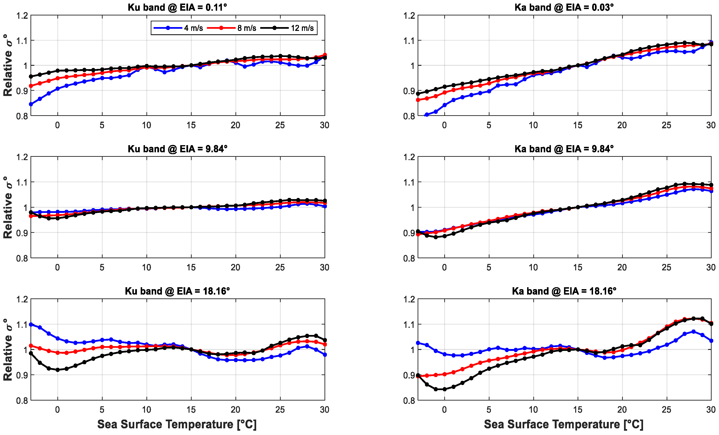
Thus, the dependence of σ
0 on SST was empirically characterized for both Ku- and Ka-bands as a function of EIA, WS and WD, using the following statistical procedure. For the EIA investigation, the σ
0 values, in linear power ratio units, were bin averaged (over all WS and WD) in 1 °C steps of SST 0–30 °C. Next, the binned averages were normalized to the corresponding σ
0 values at 15 C, and results presented in
Figure 20 show that there is an approximately linear dependence of the relative σ
0 on SST that is independent of EIA beam positions at both frequencies. However, as expected, the SST dependency is significantly stronger (> 2 x slope) for Ka band. For example, for an EIA = 9°, the overall variation of mean σ
0 with SST over the range 0–30 °C is < ± 5% at Ku, whereas it is > ± 10% for Ka.
Next, these SST binned normalized σ
0 data were sorted and averaged (separately for Ku and Ka) over WS values of 4, 8 and 12 m/s ranges, and the results are presented in
Figure 21 for EIAs of 0.1°, 9.8° and 18.6°. Here, the results are similar to
Figure 20 (averaged over all WS); however, there is also a slight WS dependence as noted by the separation of the curves. This is especially notable at the higher EIA that we suspect may be attributed to the WD effects presented next.
Next, changes in the GMF relative wind direction response due to SST were assessed using σ
0 data (not normalized), but here only the outer most beam position (EIA = 18°) was selected since it has the largest anisotropy. The results are shown in
Figure 22 for SST of 5 and 25 °C as a function of relative WD for WS values of 8, 10 and 12 m/s. For Ku-band, there appears to be no SST effects and the relative WD patterns are essentially identical; on the other hand, at Ka-band the effect is small but significant. It appears that the σ
0 WD pattern is unchanged except for a small increase in the mean (dc offset), which is consistent with the observation presented in
Figure 20.
Finally, the SST impacts, on the mean value of KuPR and KaPR σ
0, are presented in
Figure 23 as in set of 2D images for observed ranges of SST and WS. The color scale represents the mean σ
0 relative to corresponding σ
0 at 15 °C. As shown, for WS ~> 5 m/s, the mean backscatter at both band increases with SST; however, the contrast is significantly higher at Ka-band. For WS ~< 5 m/s, the trend is opposite at both bands. These SST dependent relative weights can be used as a correction factor to account for the SST impacts on the GMF. One such approach was used by [
28] to correct and validate NSCAT-5 GMF. For the DPR model of this paper (Equation (2)), this can be implemented as follows,
where
is σ
0 model in linear scale, and W is SST-impact correction factor which can determined from the tables such as presented in
Figure 23 for different EIA beam positions. Sample correction factors,
for Ku- and Ka-band models at EIA = 18° are given in the
Table A5 and
Table A6, respectively, in
Appendix B.


