A Moving Target Velocity Estimation Method Based on the MC-MASA SAR Mode

Abstract

Imaging position shift based on the multiple azimuth squint angles (MASA) mode is effective for target azimuth velocity estimation, whereas accuracy is low when target range velocity is high. In this paper, the estimation problem for both target azimuth and range velocities is considered based on the multi-channels MASA (MC-MASA) mode. Firstly, the acquisition geometry of MC-MASA mode and Doppler characteristics of a moving target are analyzed in detail, especially in squint mode. Then, for better moving target estimation, the stationary background clutter is removed using the displacement phase center antenna (DPCA) technique, and the failure in range velocity estimation with sequential SAR images is also discussed. Furthermore, a modified along-track interferometry (ATI) is proposed to preliminarily reconstruct the azimuth-and-range velocity map based on the MC-MASA mode. Since the velocity estimation accuracy is dependent on squint angle and signal-to-clutter ratio (SCR), the circumstances are divided into three cases with different iteration estimation strategies, which could expand the scene application scope of velocity estimation and achieve a high estimation accuracy along both azimuth and range directions. Finally, the performance of the proposed method is demonstrated by experimental results.

1. Introduction

Ground moving target indication (GMTI) and track formation have received growing attention in both civilian and military applications [1,2,3], with the development of synthetic aperture radar (SAR) technique. However, moving targets are defocused and dislocated in SAR image due to unknown motion parameters [4], especially in the case of long dwell time. Therefore, velocity estimation is very important for moving target imaging, as well as track generation.

Target motion introduces variations in both Doppler spectrum and range cell migration (RCM) [5,6,7], which will result in target position shift and resolution distortion in SAR image. Moreover, the effect on SAR image is different in side-looking and azimuth squint-looking. In side-looking, target motion in the range direction leads to shift of Doppler centroid frequency, which in turn results in azimuth dislocation and extra RCM. Target motion in the azimuth direction will mainly introduce Doppler frequency modulated rate variation, leading to image defocusing [8]. However, in azimuth squint-looking, both range and azimuth motions have influence on azimuth dislocation and defocusing, providing a new challenge for velocity map reconstruction.

Based on the effects mentioned above, several methods were proposed [9,10,11,12,13,14]. A GMTI approach using the reflectivity displacement method (RDM) was proposed [9] by analyzing the frequency shift and evaluating of Doppler Rate Map with high target radar cross section, where the Doppler Rate variation and range cell migration (RCM) were used for azimuth velocity and range velocity determination, respectively. Additionally, more efficient RCM evaluation was carried out with geometry-information-aided Radon transform for range velocity estimation in [10]; more accurate two-dimension search methods based on velocity correlation function (VCF) [11,12] and different geometrical figures due to target velocity vectors [13] were analyzed with high computational complexity. In order to obtain better moving target imaging quality in high-resolution SAR system, the higher-order motion parameters could be estimated based on the polynomial phase signal (PPS) model [14,15,16] and the Hough-high-order ambiguity function transform [17]. However, the estimation performance of these methods would deteriorate in the case of low signal-to-clutter ratio (SCR) and PPS model is sensitive to RCM effects.

To improve the estimation accuracy, based on the multiple-channel receiving technique, three classic methods were developed, including displacement phase center antenna (DPCA) [18], along-track interferometry (ATI) [19], and space time adaptive processing (STAP) [20], with more degrees of freedom to detect moving targets. For the DPCA method, the stationary background clutter is removed by subtracting signals from different receiving channels. By interference processing using signals from different receiving channels, the residual phase is used for target range velocity estimation, whereas the detection performance eventually depends on the signal-to-clutter-plus-noise ratio (SCNR). To address this issue, detectors were constructed by combining amplitude and phase of ATI information [21,22]. As for the STAP method, it has the best performance in theory. However, it is very time-consuming and difficult to implement in practice. Furthermore, a new Doppler-DPCA and Doppler-ATI method was developed in [23], measuring temporal Doppler shift with ultra-narrowband continuous waveforms instead of range in the conventional wideband SAR system. However, all the aforementioned methods suffer from the problem of velocity ambiguity and are incapable of azimuth velocity estimation in side-looking mode. The dual-beam ATI employed with a pair of antennas each producing a forward and an aft beam in a single pass could resolve surface velocity vector estimate of slow ocean current [24] with low spatial resolution, which is not effective for relatively small-size moving ships and vehicles detection especially with strong stationary clutter.

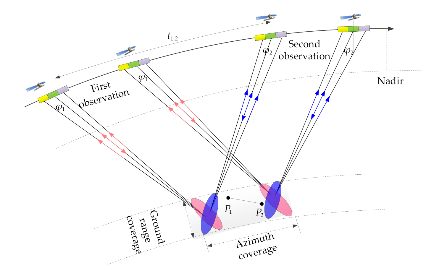
Recently, two innovative methods were studied based on sequential SAR images [25,26,27,28,29,30], including the bi-directional (BiDi) mode [25,26,27,28,29] and the multiple azimuth squint angle (MASA) mode [30]. The BiDi mode works with two main lobes pointing to different directions simultaneously in azimuth, and the same area is observed twice with a short time lag between two acquisitions. However, the pulse repetition frequency (PRF) have to be doubled for distinguishing the signal from two different directions in the azimuth frequency domain, with the range-swath reduced in half, which is undesirable for earth observing. To overcome this shortcoming, a novel MASA mode was proposed, observing the same area from different azimuth squint angles, without PRF increasing. Nevertheless, the MASA mode is only suitable for target azimuth velocity estimation. According to the analysis in [30], the effect of range motion on azimuth velocity estimation is negligible when azimuth squint angles’ absolute value of two acquisitions is equal to each other, whereas most SAR systems cannot strictly meet this requirement. Therefore, the azimuth velocity estimation accuracy deteriorates with an unknown range velocity, especially when target moves fast along the range direction. In addition, moving targets could even be buried in stationary background clutters and cannot be distinguished, and this issue has not been considered yet. Therefore, there is a need to deal with the effects on azimuth velocity estimation caused by unknown range velocity and strong stationary clutter.

In this paper, a novel velocity estimation method is proposed based on multi-channels MASA (MC-MASA) mode, which introduces multiple-channel receiving technique on MASA mode. On this basis, the DPCA technique in azimuth squint-looking is introduced for background clutter remove, which has better performance on azimuth velocity estimation with sequential SAR images. However, the range velocity estimation accuracy is low based on MASA mode with imaging position offset no matter along azimuth or range direction. For target azimuth-and-range velocity preliminarily reconstruction, the interferometric phase of ATI related to the target line-of-sight velocity is adopted with at least two acquisitions. Additionally, the detectable velocity range is double after DPCA process compared with that before clutter suppression, which could improve velocity ambiguity. However, the ATI method becomes ineffective when moving target energy is suppressed together with stationary clutter at some certain velocity and squint angle combinations. Therefore, in order to achieve a high target azimuth-and-range velocity map reconstruction accuracy even in some relatively complex situations, the circumstances are divided into three cases with different iterative strategies according to SAR acquisitions, i.e., iterative combinations of the method with moving target position shift among sequential SAR images and ATI interferometric method. The iterative strategies could also make up the blind spots of velocity estimation based on the traditional ATI method and MASA mode. Finally, the performance of the proposed method is demonstrated by experimental results.

This paper is organized as follows: In Section 2, the MC-MASA mode is presented, as well as an analysis of target motion effects on SAR image. In Section 3, based on the MC-MASA mode, the background clutter suppression method is introduced. In Section 4 and Section 5, azimuth velocity and range velocity estimation methods are derived and analyzed in detail. Experimental results are provided in Section 6 and conclusions are drawn in Section 7.

2. MC-MASA Imaging Mode

In this section, the MC-MASA mode is introduced, taking three receiving channels as an example. Compared with the MASA mode, the simultaneous slant range and Doppler spectrum variation among different channels are discussed in detail, providing the theoretical foundation for stationary clutter suppression and target velocity estimation.

2.1. Geometry Configuration

The MC-MASA geometry is shown in Figure 1, taking two observations and three receiving channels aligned in the flying direction of the SAR platform for example. The same area is observed twice with different azimuth squint angle ${\phi }_1$ and ${\phi }_2$, obtaining sequential SAR images with a time-lag $t_{1,2}$. During the time-lag between two observations, target moves from position $P_1$ to $P_2$. Therefore, the moving target will appear at different positions on sequential SAR images. Actually, six echoes of three channels observing the same scene during two separate time are obtained in Figure 1 which is different from MASA mode, providing more freedom of signal processing.

Multi-receiving channel mode results in different instantaneous slant range variation of each channel during one observation as shown in Figure 2. The distance of channel equivalent phase center (CEPC) between the three receiving channels (center of yellow, blue and purple rectangles in Figure 1) and the reference transmitting channel (center of the whole antenna) is $d_i,0,d_j$, respectively. The platform flies along the azimuth direction with velocity $V_s$. The target moves with a constant ground azimuth velocity $v_a$ and ground range velocity $v_r$ on the horizontal plane. At azimuth reference time $t=0$, three CEPCs and the moving target are at $O_i,O_0,O_j$ and $A_0$, respectively. After a time lag $t$, they move to $O_i^{\prime },O_0^{\prime },O_j^{\prime }$ and $A_1$. $R_0$ is the reference slant range between reference CEPC $i$ and moving target at $t=0$. Then, the instantaneous slant range between CEPC $i$ and moving target can be written as (1), of which $\theta$ and $\phi$ are elevation and azimuth squint angles, respectively.

$$\begin{array}{ll}{R}_i\left(t\right)& =\sqrt{{\left(V_{s}t-v_{a}t-R_0\sin \phi +d_i\right)}^2+{\left(R_0\cos \phi \sin \theta +v_{r}t\right)}^2+{\left(R_0\cos \phi \cos \theta \right)}^2}\\ & =\sqrt{R_{i0}^2+{\left(V_{s}t-v_{a}t\right)}^2+2\left(V_{s}t-v_{a}t\right)\left(-R_0\sin \phi +d_i\right)+{\left(v_{r}t\right)}^2+2R_0\cos \phi \sin \theta v_{r}t}\end{array}$$

(1)

where $R_{i0}=\sqrt{R_0{}^2+d_i^2-2R_0{d}_i\sin \phi }$ is the range between CEPC $i$ and target at $t=0$. In side-looking, the difference between $R_{i0}$ and $R_0$ is basically zero and can be neglected, whereas as squint angle $\phi$ increases, it becomes larger and should be compensated. For targets locating at other azimuth position different from $A_0$, there is only an azimuth time shift in (1) not influencing the subsequent analysis. For targets at other range cell, the reference slant range $R_0$ is varied. Therefore, Equation (1) is universally applicable for all moving targets in the observed scene.

2.2. Doppler Characteristic of Moving Target

Based on the MC-MASA mode, the range history variation no matter caused by CEPC interval or target motion is more complicated compared with side-looking mode. These variations are the basis for stationary clutter suppression and moving target velocity estimation. Therefore, it is crucial to analyze the effects of CEPC interval and target motion on Doppler spectrum and the corresponding variations.

According to Equation (1), Doppler centroid frequency $f_d$ and Doppler frequency modulated rate $f_r$ are given,

$$f_d\approx \frac{2}{\lambda }\left[\frac{-R_0\sin \phi +d_i}{R_0}{V}_s+v_{er}-v_a\frac{d_i}{R_0}\right]$$

(2)

$$f_r\approx \frac{2}{\lambda R_0}{\left(V_s\cos \phi -v_{ea}-v_r\sin \theta \frac{d_i}{R_0}\right)}^2+\frac{2}{\lambda R_0}{v}_r^2{\cos }^2\theta {\left(1-\frac{d_i}{R_0}\sin \phi \right)}^2$$

(3)

where $\lambda$ is the wavelength.

Considering the squint observation, $v_{ea},v_{er}$ are defined as equivalent azimuth velocity (EAV) and equivalent range velocity (ERV), respectively,

$$v_{ea}=v_a\cos \phi -v_r\sin \theta \sin \phi$$

(4a)

$$v_{er}=v_a\sin \phi +v_r\sin \theta \cos \phi$$

(4b)

Here, the line of radar sight is defined as equivalent range direction and the corresponding perpendicular direction is equivalent azimuth direction, as shown by the green line and blue line in Figure 2, along which the velocity is $V_s\sin \phi$ and $V_s\cos \phi$ respectively.

Then, $f_d$ and $f_r$ can be rewritten as follows,

$$f_d=f_d{}_0+f_{d,V_s,i}+f_{d,v_a}+f_{d,v_r}$$

(5)

$$f_r=f_r{}_0+f_{r,v_a}+f_{r,v_r}+f_{r,v_a,v_r}$$

(6)

where $f_d{}_0$, $f_{d,v_a}$ and $f_{d,v_r}$ are Doppler centroid frequency caused by the platform movement and target movement along azimuth and range directions, respectively. $f_r{}_0$, $f_{r,v_a}$ and $f_{r,v_r}$ are the corresponding Doppler frequency modulated rate. $f_{d,V_s,i}$ is Doppler centroid frequency dependent on $d_i$ and $f_{r,v_a,v_r}$ is the united motion influence caused by target coupled azimuth and range velocity.

$$f_{d0}=-2V_s\sin \phi /\lambda$$

(7a)

$$f_{d,V_s,i}=2V_s{d}_i/\left(\lambda R_0\right)$$

(7b)

$$f_{d,v_a}=2v_a\sin \phi /\lambda -2v_a{d}_i/\left(\lambda R_0\right)\approx 2v_a\sin \phi /\lambda$$

(7c)

$$f_{d,v_r}=2v_r\sin \theta \cos \phi /\lambda$$

(7d)

$$f_{r0}=2V_s{}^2{\cos }^2\phi /\left(\lambda R_0\right)$$

(8a)

$$f_{r,v_a}=2\left(-2V_s{v}_a+v_a{}^2\right){\cos }^2\phi /\left(\lambda R_0\right)\approx -4V_s{v}_a{\cos }^2\phi /\left(\lambda R_0\right)$$

(8b)

$$f_{r,v_r}\approx \frac{4}{\lambda R_0}{V}_s{v}_r\sin \theta \left(\sin \phi -d_i/R_0\right)\cos \phi +\frac{2}{\lambda R_0}\left(v_r{}^2{\sin }^2\theta {\sin }^2\phi +v_r^2{\cos }^2\theta \right)\approx 2V_s{v}_r\sin \theta \sin \left(2\phi \right)/\left(\lambda R_0\right)$$

(8c)

$$f_{r,v_a,v_r}=4v_a{v}_r\sin \theta \left(d_i/R_0-\sin \phi \right)\cos \phi /\left(\lambda R_0\right)$$

(8d)

For simplicity and without affecting the subsequent analysis, the Doppler spectrum shifts caused by target motion and CEPC interval are ignored in Equations (7c), (8b) and (8c), whose values are very close to zero. Consequently, the variation of $f_d$ and $f_r$ caused by target azimuth and range motion can be analyzed individually based on Equations (7) and (8). Figure 3 shows these variations with different azimuth squint angles, using parameters listed in

Table 1. Simulation parameters.

Parameter	Value	Parameter	Value
Wavelength	0.03 m	Orbit Height	550 km
Elevation	${32}^{°}$	$d_{-1}$	−2.8 m
PRF	3000 Hz	$d_0$	0
Platform Velocity (m/s)	7500 m/s	$d_1$	2.8 m

.

In comparison to the stationary clutter, the effects of $f_d$ and $f_r$ variation on azimuth and slant range directions are analyzed as follows.

(1) Azimuth time offset

$$\Delta t=f_{d0}/f_{r0}-f_d/f_r\approx -\Delta f_d/f_{r0}$$

(9a)

$$\Delta t_{v_a}=-f_{d,v_a}/f_{r0}\approx -R_0{v}_a\sin \phi /\left(V_s^2{\cos }^2\phi \right)$$

(9b)

$$\Delta t_{v_r}=-f_{d,v_r}/f_{r0}\approx -R_0{v}_r\sin \theta /\left(V_s^2\cos \phi \right)$$

(9c)

where $\Delta t$ is the azimuth time offset due to Doppler spectrum shift, and $\Delta t_{v_a}$ and $\Delta t_{v_r}$ are caused by target azimuth and range motions, respectively; $\Delta f_d=f_{d,v_a}+f_{d,v_r}$.

(2) Slant range offset

$$\Delta R=-\frac{\lambda }{2}\left(f_{d0}+\frac{\Delta f_d}{2}\right)\frac{\Delta f_d}{f_{r0}}$$

(10a)

$$\Delta R_{v_a}\approx \frac{R_0\left(V_s-v_a/2\right)v_a{\sin }^2\phi }{V_s^2{\cos }^2\phi }$$

(10b)

$$\Delta R_{v_r}\approx \frac{R_0{v}_r\sin \theta \sin \phi }{V_s\cos \phi }-\frac{R_0{v}_r^2{\sin }^2\theta }{2V_s^2}$$

(10c)

where $\Delta R$ is the slant range offset due to Doppler spectrum shift, and $\Delta R_{v_a}$ and $\Delta R_{v_r}$ are caused by target azimuth and range motions, respectively.

According to Equation (9), the azimuth position offset caused by target azimuth motion is linear and changes obviously as squint angle varies, which has been adopted for azimuth velocity estimation in [30]. Similarly, linear offset of range history caused by range motion as Equation (10) may also provide a possibility for range velocity estimation based on sequential SAR images, which will be further explained later. However, moving target could be submerged in stationary clutters, not distinguishable when its energy is lower than stationary clutters. Especially in complicated urban areas, the vehicles may be imaged in the strong building region and cannot be identified. This explains that the application scope of the method based on image position shift is just restricted to high SCR. Stationary clutter suppression could not only expand the application scope of this method in case of low SCR, but also makes the target contour clearer improving moving target recognition accuracy. Therefore, clutter remove is the prerequisite of target velocity extraction which would be analyzed firstly in Section 3.

3. Background Clutter Suppression

In this section, a background clutter suppression method is presented based on the MC-MASA mode with squint observation.

After range pulse compression, the azimuth signal for receiving channel $i$ can be represented as,

$$\begin{array}{ll}{s}_i\left(t\right)& =A{\omega }_a\left(t\right)\exp \left\{-j2\pi \left[R_0\left(t\right)+R_i\left(t\right)\right]/\lambda \right\}\\ & \approx A{\omega }_a\left(t\right)\exp \left\{-j2\pi \left[\left(R_0+R_{i0}\right)/\lambda +f_{d0}t+f_{d,V_s,i}t/2\right]\right\}\exp \left\{-j2\pi \left[\Delta f_{d}t+\left(f_{r0}+\Delta f_r\right)t^2/2\right]\right\}\end{array}$$

(11)

where $A$ is the target complex reflectivity, ${\omega }_a\left(t\right)$ denotes the azimuth window function and $\Delta f_r=f_{r,v_a}+f_{r,v_r}$. In moderate-resolution SAR system, the higher order terms ($\ge 3$) of slant range influence little which could be neglected. Even if in the high-resolution SAR system, some higher order terms could be compensated during clutter suppression as the effect of target motion on them is small. Therefore, the approximation in Equation (11) is meaningful in the following analysis.

Target energy will be focused after pulse compression with increased signal-to-noise ratio (SNR) which is beneficial for velocity estimation. Based on the principle of stationary phase (POSP), the signal in the azimuth-frequency domain is

$$S_i\left(f\right)=A{\omega }_a\left[-\frac{f+f_{d0}}{f_{r0}}\right]\exp \left\{-j2\pi \frac{R_0+R_{i0}}{\lambda }\right\}\exp \left\{j\pi \frac{{\left(f+f_{d0}+\Delta f_d+f_{d,V_s,i}/2\right)}^2}{f_{r0}+\Delta f_r}\right\}$$

(12)

where $f$ denotes azimuth frequency variable with respect to the azimuth time variable.

In some classic SAR image formation algorithms, such as the range Doppler algorithm (RDA) [31], the chirp scaling algorithm (CSA) [32], and the deramp chirp scaling algorithm (DCS) [33], the azimuth position of target on a SAR image is usually at the time corresponding to Doppler centroid frequency. Consequently, the azimuth matched filtering function for azimuth signal compression is constructed as,

$$H_{match}\left(f\right)=\exp \left\{-j\pi {\left(f+f_{d0}\right)}^2/f_{r0}\right\}$$

(13)

After multiplying $H_{match}\left(f\right)$ by $S_i\left(f\right)$ in Equation (12), one has

$$\begin{array}{ll}{S}_{i2}\left(f^{\prime }\right)& =A{\omega }_a\left(-\frac{f^{\prime }}{f_{r0}}\right)\exp \left\{-j2\pi \left(\frac{R_0+R_{i0}}{\lambda }\right)\right\}\\ & \cdot \exp \left\{j\pi \frac{f^{\prime }{f}_{d,V_s,i}+\Delta f_d^2+f_{d,V_s,i}^2/4}{f_{r0}+\Delta f_r}\right\}\exp \left\{j\pi \frac{2\Delta f_d\left(f^{\prime }+f_{d,V_s,i}/2\right)f_{r0}-f^{\prime }{}^2\Delta f_r}{\left(f_{r0}+\Delta f_r\right)f_{r0}}\right\}\end{array}$$

(14)

where $f^{\prime }=f+f_{d0}$ denotes the equivalent azimuth frequency after frequency shift.

In order to compensate for the variation of receiving signal due to the CEPC interval, the following azimuth compensation filtering function is employed

$$H_{com}\left(f^{\prime }\right)=\exp \left\{-j2\pi \left[\frac{R_0-R_{i0}}{\lambda }+\frac{f^{\prime }{f}_{d,V_s,i}}{2f_{r0}}+\frac{f_{d,V_s,i}^2}{8f_{r0}}\right]\right\}$$

(15)

Discrete processing in the frequency domain incurs a small error when $N_a{f}_{d_0}/f_{prf}$ is not an integer and the maximum phase error of channel $i$ can be deduced as

$${\left|\Delta \alpha \right|}_{\max }=\pi f_{prf}{f}_{d.V_s,i}/\left(2N_a{f}_{r0}\right)\approx 0$$

(16)

where $f_{prf}$ is PRF of the system and $N_a$ is the number of azimuth pulses. However, in the azimuth time domain, $\Delta t_i=f_{d,V_s,i}/f_{r0}=m/f_{prf}$ ($m$ is an integer) is required for compensating for the variation between different channels commented as DPCA condition, which is not necessary in the frequency domain. When $\Delta t_i\ne m/f_{prf}$, the time-consuming interpolation operation is needed. Therefore, it is computationally efficient to perform the processing in the frequency domain without interpolation.

With phase compensation, the signal is transformed to

$$S_{is}\left(f^{\prime }\right)\approx A{\omega }_a\left(-\frac{f^{\prime }}{f_{r0}}\right)\exp \left\{-j\pi \left(\frac{4R_0}{\lambda }+\frac{f^{\prime }{}^2\Delta f_r}{f_{r0}^2}\right)\right\}\exp \left\{j\pi \frac{\Delta f_d\left(\Delta f_d+f_{d,V_s,i}\right)+2\Delta f_d{f}^{\prime }}{f_{r0}}\right\}$$

(17)

After performing azimuth IFFT,

$$s_{is}\left(t\right)=A{G}_a{P}_a\left(t+\frac{\Delta f_d}{f_{r0}}\right)\exp \left\{-j\pi \left(\frac{4R_0}{\lambda }-\frac{\Delta f_d^2+\Delta f_d{f}_{d,V_s,i}}{f_{r0}}\right)\right\}$$

(18)

where $G_a$ denotes compression gain of azimuth and $P_a\left(•\right)$ is product of the envelope of ${\omega }_a\left(•\right)$ after pulse compression and the influence of defocusing, whose amplitude can be assumed as a $\sin c\left(·\right)$ function, and then the moving target will be well focused at $t=-\Delta f_d/f_{r0}$ as Equation (9a). The defocusing effect is considered in Section 6.

Afterwards, stationary clutters can be removed by subtracting acquisitions from different channels. Taking channels $i$ and $j$ as an example, one has

$$s_{ij}^{DPCA}\left(t\right)=s_{is}\left(t\right)-s_{js}\left(t\right)=A{G}_a{P}_a\left(t+\Delta f_d/f_{r0}\right)\exp \left(j{\theta }_i\right)\left(1-\exp \left(j{\Theta }_{ij}\right)\right)$$

(19)

where

$${\theta }_i=-4\pi R_0/\lambda +\pi \left(\Delta f_d^2+\Delta f_d{f}_{d,V_s,i}\right)/f_{r0}$$

(20a)

$${\Theta }_{ij}={\theta }_i-{\theta }_j=\pi \Delta f_d\left(f_{d,V_s,j}-f_{d,V_s,i}\right)/f_{r0}$$

(20b)

Thus

$$\left|s_{ij}^{DPCA}\left(t\right)\right|=A{G}_a\left|2\sin \left({\Theta }_{ij}/2\right)\right|=A{G}_a\left|2\sin \left[\pi v_{er}{d}_{ij}/\lambda V_s{\cos }^2\phi \right]\right|$$

(21)

where $d_{ij}=d_i-d_j$.

It can be seen from Equation (21) that the stationary clutters would be removed as ${\Theta }_{ij}=0$ and the residual intensity of moving target varies with target ERV after DPCA processing. Unless the residual phase ${\Theta }_{ij}$ of moving target is proportional to $2\pi$, moving target could be retained and identified. Different from the side-looking mode where the residual target intensity is related to target range velocity, the intensity is dependent on target ERV in squint-looking. In other words, the moving target would be subtracted together with clutter when $v_{er}=0$ even if the target has velocity both along azimuth and range direction. This characteristic makes the subsequent velocity estimation complicated and diversified with different SAR acquisition combinations which would be discussed in Section 5. Generally, moving target would be more obvious after DPCA process and this is beneficial for the estimation method based on target imaging information in Section 4.

4. Azimuth Velocity Estimation Based on Position Offset

In this section, target azimuth velocity estimation based on the azimuth image position offset is analyzed in detail and the failure for range velocity estimation based on image position offset is also addressed.

4.1. Azimuth Position Offset

Azimuth pixel offset of a moving target due to mismatch of Doppler centroid frequency is

$$\Delta N=-f_{prf}\Delta f_d/f_{r0}$$

(22)

Consequently, the azimuth pixel offset between two sequential SAR images of squint angle ${\phi }_k$ and ${\phi }_m$ can be deduced as follows,

$$\Delta N\left(k,m\right)=\Delta N\left(m\right)-\Delta N\left(k\right)+\Delta N_{k\to m}$$

(23)

where $\Delta N_{k\to m}\approx v_a{f}_{prf}\left(R_k\sin {\phi }_k-R_m\sin {\phi }_m\right)/V_s{}^2$ is the azimuth pixel offset during these two observations due to target azimuth motion. $R_k$ and $R_m$ represent the reference slant range corresponding to the squint angle ${\phi }_k$ and ${\phi }_m$, respectively.

As mentioned in Section 2, both target azimuth and range velocities will cause azimuth position offset without coupling with each other. Then, $\Delta N\left(k,m\right)$ can be divided into

$$\Delta N\left(k,m\right)=\Delta N{\left(k,m\right)}_{v_a}+\Delta N{\left(k,m\right)}_{v_r}$$

(24)

$$\Delta N{\left(k,m\right)}_{v_a}=\frac{v_a{f}_{prf}}{V_s{}^2}\times \frac{R_k\sin {\phi }_k\left(1+{\cos }^2{\phi }_k\right)}{{\cos }^2{\phi }_k}-\frac{v_a{f}_{prf}}{V_s{}^2}\times \frac{R_m\sin {\phi }_m\left(1+{\cos }^2{\phi }_m\right)}{{\cos }^2{\phi }_m}$$

(25)

$$\Delta N{\left(k,m\right)}_{v_r}=\frac{v_r\sin \theta f_{prf}}{V_s^2}\left(\frac{R_k}{\cos {\phi }_k}-\frac{R_m}{\cos {\phi }_m}\right)$$

(26)

where $\Delta N{\left(k,m\right)}_{v_a}$ and $\Delta N{\left(k,m\right)}_{v_r}$ are the azimuth pixel offset caused by target azimuth and range motions, respectively.

With unknown range velocity, the azimuth velocity can be deduced as

$${\widehat{v}}_a\left(k,m\right)=\frac{\Delta N\left(k,m\right)}{\frac{R_k\sin {\phi }_k\left(1+{\cos }^2{\phi }_k\right)}{{\cos }^2{\phi }_k}-\frac{R_m\sin {\phi }_m\left(1+{\cos }^2{\phi }_m\right)}{{\cos }^2{\phi }_m}}\frac{V_s^2}{f_{prf}}$$

(27)

$${\widehat{v}}_a{\left(k,m\right)}_{err\_v_r}=\frac{\left(R_k\cos {\phi }_m-R_m\cos {\phi }_k\right)v_r\sin \theta }{\frac{R_k\sin {\phi }_k\left(1+{\cos }^2{\phi }_k\right)}{\cos {\phi }_k}\cos {\phi }_m-\frac{R_m\sin {\phi }_m\left(1+{\cos }^2{\phi }_m\right)}{\cos {\phi }_m}\cos {\phi }_k}$$

(28)

where ${\widehat{v}}_a{\left(k,m\right)}_{err\_v_r}$ is the estimation error due to the unknown range velocity.

Analyzing Equation (28), with the same absolute value of the squint angles, i.e., ${\phi }_m=-{\phi }_k$, azimuth velocity estimation error is very small caused by target range motion, so ${\widehat{v}}_a\left(k,m\right)$ can be rewritten as

$${\widehat{v}}_a\left(k,-k\right)=\frac{\Delta N\left(k,-k\right)}{2R_k\sin {\phi }_k\left(1+{\cos }^2{\phi }_k\right)}\frac{V_s^2{\cos }^2{\phi }_k}{f_{prf}}$$

(29)

However, if the absolute values of squint angles are not equal to each other, the azimuth velocity estimation error caused by target range motion cannot be ignored as shown in Figure 4, with parameters listed in Table 1. In Figure 4a, the azimuth pixel offset with different combinations of squint angles is given, on the condition of target range motion 20 m/s and 40 m/s, respectively. As shown, the larger the difference in the absolute value of squint angle is, the larger the azimuth pixel offset becomes. Furthermore, the corresponding azimuth velocity estimation errors caused by range velocity are provided in Figure 4b, which should be considered especially when the absolute values of squint angles are not the same.

Notice that although range motion is the dominant factor in azimuth position offset on one SAR image, position deviation among sequential images is small. As shown in Figure 4a, a 40 m/s range velocity only causes offset of about six azimuth pixels with the combination $\left(5^{°},0\right)$, meaning that one-pixel registration error leads to an estimation error of about 6m/s. Additionally, when range velocity is lower than 6m/s, there is less than one pixel offset which is hard to be distinguished. Therefore, the method based on azimuth position offset is not effective enough for range velocity estimation.

4.2. Slant Range Offset due to Range Velocity

Except for azimuth position offset, the mismatch of Doppler spectrum also causes extra slant range offset as in Equation (10). The slant range offset between acquisitions of squint angle ${\phi }_k$ and ${\phi }_m$ is

$$\Delta R\left(k,m\right)=\Delta R\left(m\right)-\Delta R\left(k\right)+\Delta R_{k\to m}$$

(30)

where $\Delta R_{k\to m}=v_r\left(R_k\sin {\phi }_k-R_m\sin {\phi }_m\right)/V_s$ is the range offset during these two observations due to target range motion. $\Delta R\left(k\right)$ and $\Delta R\left(m\right)$ are range offset with squint angle ${\phi }_k$ and ${\phi }_m$, respectively.

Substituting Equation (10c) into Equation (30), the range migration arising from range velocity is given by

$$\Delta R{\left(k,m\right)}_{v_r}=\frac{v_r^2\left(R_k-R_m\right)}{2V_s^2}+\frac{v_r\sin \theta R_k\sin {\phi }_k\left(\cos {\phi }_k-1\right)}{V_s\cos {\phi }_k}-\frac{v_r\sin \theta R_m\sin {\phi }_m\left(\cos {\phi }_m-1\right)}{V_s\cos {\phi }_m}$$

(31)

According to Equation (31), Figure 5 illustrates range offset arising from range velocity, using parameters listed in Table 1. Although the range offset caused by range motion in one image is large, the deviation between two images is much smaller than image resolution as shown in Figure 5a,b, making it difficult to be identified. This is because the offset during two acquisitions $\Delta R_{k\to m}$ almost equals the deviation between two images as $\Delta R\left(k\right)-\Delta R\left(m\right)$. Therefore, since the relative image position offset is small along both azimuth and range directions, the method based on sequential SAR images is incapable of range velocity estimation.

5. Azimuth-and-Range Velocity Estimation Based on MC-MASA Mode

As discussed in Section 4, target range velocity cannot be obtained based on image position offset, and the unknown range velocity affects estimation accuracy of azimuth velocity seriously. Therefore, based on the MC-MASA mode, a novel ATI technique is introduced and discussed in detail to reconstruct the azimuth-and-range velocity map after clutter removal in this section. Its performance is analyzed by considering interferometric phase and system parameters. Finally, according to the obtained SAR acquisitions and residual target energy, the circumstances are divided into three cases with different iterative estimation strategies.

5.1. Target Azimuth-and-Range Velocity Estimation

By multiplying a complex conjugate of one image with the other image, the interferogram from channels $i$ and $j$ is obtained as

$$s_{ij}^{ATI}\left(t\right)=s_{is}\left(t\right)s_{js}^{*}\left(t\right)=A{G}_a{P}_a\left(t+\Delta f_d/f_{r0}\right)\exp \left\{j2\pi v_{er}{d}_{ij}/\left(\lambda V_s{\cos }^2\phi \right)\right\}$$

(32)

where “*” denotes the complex conjugate.

Then, interferometric phase ${\varphi }_{ij}$ and ERV estimation result ${\widehat{v}}_{er}^{ATI}\left(\phi \right)$ are given by

$${\varphi }_{ij}=2\pi v_{er}{d}_{ij}/\left(\lambda V_s{\cos }^2\phi \right)$$

(33)

$${\widehat{v}}_{er}^{ATI}\left(\phi \right)={\varphi }_{ij}\lambda V_s{\cos }^2\phi /\left(2\pi d_{ij}\right)$$

(34)

The obtained ERV contains both target azimuth and range velocities because of their interaction on the linear term of range history in azimuth squint-looking, which is different from side-looking. However, clutters would severely affect the interferometric phase of moving targets, degrading the estimation accuracy. In the worst situation, when moving target is totally submerged in background clutters, velocity estimation methods based on ATI only will fail. Fortunately, the signal after DPCA retains the phase information of moving targets, i.e., Equation (19) has all the phase information of a moving target in Equation (18). Therefore, interferometric processing of two acquisitions after clutter suppression is also effective for target velocity estimation. These two acquisitions are based on signals from three receiving channels of which every two are processed with DPCA. However, only amplitude with DPCA or interferometric phase with ATI can be obtained with dual-channel signals from which the velocity of moving targets is difficult to be estimated in low SCR.

Taking channels $\left(i,j,p\right)$ for example, two images $s_{ij}^{DPCA}\left(t\right)$ and $s_{ip}^{DPCA}\left(t\right)$ after clutter suppression are obtained from channel $i,j$ and channel $i,p$, respectively. Then, the interferogram is expressed as

$$s_{DPCA}^{ATI}\left(t\right)=s_{ij}^{DPCA}\left(t\right)\times s_{ip}^{DPC{A}^{*}}\left(t\right)$$

(35)

According to Equation (35), phase ${\Phi }_{jp}$ and the estimated ERV ${\widehat{v}}_{er}\left(\phi \right)$ based on DPCA-ATI can be deduced as

$${\Phi }_{jp}=\pi v_{er}{d}_{jp}/\left(\lambda V_s{\cos }^2\phi \right)$$

(36)

$${\widehat{v}}_{er}\left(\phi \right)={\Phi }_{jp}\lambda V_s{\cos }^2\phi /\left(\pi d_{jp}\right)$$

(37)

From Equation (37), the estimated ERV of a certain squint angle is related to the interferometric phase of channels $j$ and $p$ after DCPA processing. The signal of channel $i$ plays an important role in clutter suppression and is cancelled during the interference process.

According to the projection relationship between the moving target equivalent velocity in the slant range plane and actual velocity in the horizontal ground plane shown in Figure 2, target azimuth and range velocities can be derived based on the combination of two ERV results with ${\phi }_k$ and ${\phi }_m$, as

$$\left[\begin{array}{c}{\widehat{v}}_a\\ {\widehat{v}}_r\end{array}\right]={\left[\begin{array}{cc}\sin {\phi }_k& \sin \theta \cos {\phi }_k\\ \sin {\phi }_m& \sin \theta \cos {\phi }_m\end{array}\right]}^{-1}\left[\begin{array}{c}{\Phi }_{jp}\lambda V_s{\cos }^2{\phi }_k/\left(\pi d_{jp}\right)\\ {\Phi }_{jp}\lambda V_s{\cos }^2{\phi }_m/\left(\pi d_{jp}\right)\end{array}\right]$$

(38)

With the increase of the azimuth steering span, more than two acquisitions can be obtained in the MC-MASA mode. Therefore, the least-square solution of an overdetermined equation is the more suitable result

$$\left[\begin{array}{l}\begin{array}{cc}\sin {\phi }_1& \sin \theta \cos {\phi }_1\\ \sin {\phi }_2& \sin \theta \cos {\phi }_2\end{array}\\ \begin{array}{cc}\dots & \dots \\ \sin {\phi }_n& \sin \theta \cos {\phi }_n\end{array}\end{array}\right]\left[\begin{array}{c}{\tilde{v}}_a\\ {\tilde{v}}_r\end{array}\right]=\left[\begin{array}{c}{\Phi }_{jp}\lambda V_s{\cos }^2{\phi }_1/\left(\pi d_{jp}\right)\\ \begin{array}{c}{\Phi }_{jp}\lambda V_s{\cos }^2{\phi }_2/\left(\pi d_{jp}\right)\\ \dots \\ {\Phi }_{jp}\lambda V_s{\cos }^2{\phi }_n/\left(\pi d_{jp}\right)\end{array}\end{array}\right]$$

(39)

where $n$ is the number of effective SAR acquisitions and ${\tilde{v}}_a,{\tilde{v}}_r$ is the estimated azimuth and range velocities, respectively.

It can be noticed that the interferometric phase after DPCA is half as before which can reduce the possibility of ambiguity velocity, i.e., the detectable ERV range is doubled. Moreover, ATI processing after DPCA can further suppress the clutter.

Phase wrapping results in target ERV ambiguity when the interferometric phase exceeds $\left[-\pi ,\pi \right]$. The maximum estimate target ERV in Equation (37) is given by

$$\left|{\widehat{v}}_{er,\max }\right|=\lambda V_s{\cos }^2\phi /d_{jp}$$

(40)

With the parameters listed in Table 1, ${\widehat{v}}_{er,\max }$ is $40 \mathrm{m}/\mathrm{s}\left(~144\mathrm{km}/\mathrm{h}\right)$ when $d_{jp}=5.6 \mathrm{m}$ and $\phi =5^{°}$. The corresponding ground velocity is basically doubled as $80 \mathrm{m}/\mathrm{s}\left(~288\mathrm{km}/\mathrm{h}\right)$. If $d_{jp}=2.8 \mathrm{m}$ is chosen, this velocity will be doubled again. Therefore, the estimated maximum ambiguity-free velocity based on the spaceborne radar system can cover the velocity of most ground and maritime moving targets. For airborne SAR system, there are three baseline combinations if the distance between CEPCs is different (noted as $d_{ij},d_{jp},d_{ip}$) in MC-MASA mode in this paper which could further expand the range of estimated velocity. Meanwhile, due to the finite ambiguity number of target velocity, several comparisons of Radon transform results of RCM [10] could resolve the problem of target ERV ambiguity with low complexity.

Target azimuth-and-range velocity reconstruction needs two observations based on the MC-MASA mode and the others can be used to further improve estimation accuracy.

5.2. Velocity Estimation Sensitivity Analysis

Interferometric phase directly determines the estimated target velocity as Equation (37), so the phase extraction method is important. Apart from phase, the sensitivity of ${\widehat{v}}_{er}\left(\phi \right)$ is also related to system parameters, such as platform velocity, CEPC interval and squint angle. These factors will be analyzed specifically. Unless otherwise stated, parameters listed in Table 1 and

Table 2. Parameters for sensitivity analysis.

Parameter	$\phi$	$d_{jp}$	${\Phi }_{jp}$
Value	$5^{°}$	5.6 m	1.57 rad

are chosen for the subsequent analysis, corresponding to ${\widehat{v}}_{er}\left(\phi \right)=20 \mathrm{m}/\mathrm{s}$.

• Sensitivity to interferometric phase ${\Phi }_{jp}$

  $$\frac{\partial \left[{\widehat{v}}_{er}\left(\phi \right)\right]}{\partial {\Phi }_{jp}}=\frac{\lambda V_s{\cos }^2\phi }{\pi d_{jp}}$$

  (41)

With the above parameters, each phase error of 0.1 rad will result in an ERV error of 1.27 m/s. After clutter suppression, the moving target can be distinguished by amplitude threshold judgment. When the extended target size is larger than one pixel on a SAR image, it will occupy multiple pixels and each point corresponds to one phase which is affected by the residual clutter at the same position. It is generally assumed that clutters are subject to Gaussian distributions, i.e., its amplitude follows the Rayleigh distribution and its phase follows the uniform distribution. Therefore, the minimum mean square error (MMSE) criterion can be used to reduce interferometric phase error by statistical analysis for this situation.

• Sensitivity to platform velocity $V_s$

  $$\frac{\partial \left[{\widehat{v}}_{er}\left(\phi \right)\right]}{\partial V_s}=\frac{{\Phi }_{jp}\lambda {\cos }^2\phi }{\pi d_{jp}}$$

  (42)

With the above parameters, each platform velocity error of 100 m/s only leads to a target ERV error of 0.27 m/s, indicating that ERV is not very sensitive to platform velocity. In spaceborne SAR, the actual path of satellite is approximated to a straight line [34], so equivalent platform velocity is adopted in SAR imaging.

• Sensitivity to squint angle $\phi$

  $$\frac{\partial \left[{\widehat{v}}_{er}\left(\phi \right)\right]}{\partial \phi }=-\frac{{\Phi }_{jp}\lambda V_s\sin 2\phi }{\pi d_{jp}}$$

  (43)

With the above parameters, each squint angle error of 0.1 rad leads to a target ERV error of −0.35 m/s and a small squint angle can decrease this error. The same for platform velocity, it is the equivalent squint angle in spaceborne SAR.

Assuming that $\Delta ER{V}_k$ and $\Delta ER{V}_m$ are the ERV estimation error of squint angle ${\phi }_k$ and ${\phi }_m$, respectively. Then, the estimation error of $v_a$ and $v_r$ can be derived as

$$\left\{\begin{array}{l}\Delta {\widehat{v}}_a=\frac{\Delta ER{V}_k\cos {\phi }_m-\Delta ER{V}_m\cos {\phi }_k}{\sin {\phi }_k\cos {\phi }_m-\sin {\phi }_m\cos {\phi }_k}\hfill \\ \Delta {\widehat{v}}_r=\frac{\Delta ER{V}_k\sin {\phi }_m-\Delta ER{V}_m\sin {\phi }_k}{\left(\sin {\phi }_m\cos {\phi }_k-\sin {\phi }_k\cos {\phi }_m\right)\sin \theta }\hfill \end{array}\right.$$

(44)

In the small squint angle mode, the azimuth velocity estimation error is larger than that of range direction in most cases, about $\cot \phi \sin \theta$ times, which is negatively correlated with the absolute value of squint angle. Therefore, combination of large squint angles should be chosen for azimuth velocity estimation under the premise of an accurate squint angle.

• Sensitivity to CEPC interval $d_{jp}$

  $$\frac{\partial \left[{\widehat{v}}_{er}\left(\phi \right)\right]}{\partial d_{jp}}=-\frac{{\Phi }_{jp}\lambda V_s{\cos }^2\phi }{\pi d_{jp}^2}$$

  (45)

With the above parameters, every interval error of 0.1 m leads to a target ERV error of −0.36 m/s and a large interval is needed for accurate ERV estimation. However, a large CEPC interval would deteriorate situation of velocity ambiguity. Therefore, the choice of $d_{jp}$ is trade-off by considering both SAR system parameters and the moving target velocity range. For higher accuracy, with the actual path of satellite is straightened, this interval also has a small approximation change. Additionally, the smaller the wavelength is, the better the accuracy is.

5.3. Estimation Process

The method based on the MASA mode in Section 4 is only capable of target azimuth velocity estimation with the same absolute values of the squint angles. Both target azimuth and range velocities can be extracted from the phase difference as aforementioned discussion, whereas estimation accuracy of azimuth velocity is poor. Therefore, these two methods could be combined to improve estimation accuracy and application scope. The estimation process should be chosen according to the situations considered. Note that in the subsequent analysis, method 1 and method 2 denote the method in Section 4 and Section 5, respectively.

In order to extract more information of moving targets, the stationary clutter is removed firstly for all acquisitions. As both method 1 and method 2 are based on two acquisitions, only two images with squint angle ${\phi }_k$ and ${\phi }_m$ are analyzed in the following cases. In addition, the relationship of squint angles is an important factor for velocity estimation. Therefore, different cases are discussed, with different corresponding processes.

• Case 1: ${\phi }_k=-{\phi }_m$

The estimated azimuth velocity ${\widehat{v}}_a$ from method 1 has a small error and range velocity ${\widehat{v}}_r$ can be extracted by method 2 from either of the two images. The worst situation is that the moving target on image ${\phi }_k$ is removed together with clutter after DPCA processing due to a nearly zero ERV. Now azimuth velocity can be estimated firstly if the targets on both images can be distinguished clearly before clutter removal. Then, range velocity is obtained from the image of ${\phi }_m$.

• Case 2: ${\phi }_k\ne -{\phi }_m$ and ERV can be extracted from both acquisitions

The ERV extraction criterion is that the interference phase of a moving target is clustered around a certain value, which will be further illustrated in subsequent simulations. The range velocity ${\widehat{v}}_{r1}$ can be firstly extracted with method 2 which can compensate the estimation error in azimuth velocity ${\widehat{v}}_{a1}$ of method 1. Finally, with an iterative process, more accurate ${\widehat{v}}_{r2}$ and ${\widehat{v}}_{a2}$ are obtained successively with method 2 and method 1, respectively.

• Case 3: ${\phi }_k\ne -{\phi }_m$ and ERV cannot be extracted from the ${\phi }_k$ acquisition

For this case, moving target can be distinguished on images of ${\phi }_k$ and ${\phi }_m$ with method 1 after clutter suppression. However, method 2 is only effective for ERV extraction with image ${\phi }_m$. The erroneous azimuth velocity ${\widehat{v}}_{a1}$ from method 1 and interferometric phase of image ${\phi }_m$ can be combined for estimation of range velocity ${\widehat{v}}_{r1}$ with method 2. Finally, with iterations, more accurate ${\widehat{v}}_{a2}$ is obtained from method 1 with compensation of range motion and then ${\widehat{v}}_{r2}$ is estimated again with method 2. If the azimuth position offset caused by ${\widehat{v}}_{r1}$ is less than half a pixel, its effect on azimuth velocity estimation of method 1 can be ignored. ${\widehat{v}}_{r1}$ and ${\widehat{v}}_{a1}$ are the final results.

In either case, when target EAV exceeds a certain threshold $v_{ea,thre}$, the moving target should be refocused, as defocusing will lead to reduction of SCR, which in turn reduces velocity estimation accuracy. Here, $v_{ea,thre}$ corresponds to the target gain attenuated by 3dB. The criterion for setting the velocity threshold $v_{ea,threshold}$ in [30] is the main lobe separation, not considering the effect of SCR. According to the parameters in Table 1, $v_{ea,thre}=11 \mathrm{m}/\mathrm{s}$ as shown in Figure 6; $v_{ea,threshold}$ is 24 m/s with resolution ${\rho }_a=3.2 \mathrm{m}$, larger than $v_{ea,thre}$.

The filter function of quadratic phase error correction in the azimuth-frequency domain is given by

$$H_{quar}(f)=\exp \left\{-j\pi \left(\frac{1}{f_r}-\frac{1}{f_{r0}}\right)f^2\right\}$$

(46)

For a small squint angle, estimation accuracy of azimuth velocity depends strongly on the squint angle, while that of range direction is hardly affected by it. Therefore, it is better to choose combinations of large squint angles for better estimation performance. Moreover, if there are more than two acquisitions, it is better to choose combinations corresponding to Case 1 with the simplest process and best accuracy.

The flowchart of the proposed method is shown in Figure 7.

6. Experimental Results

In this section, simulation results for both point target and extended target are provided.

6.1. Point Target Results

For point target, it is performed firstly with two sequential images of squint angles ${\phi }_1=5^{°}$ and ${\phi }_2=-1^{°}$ as Case 2, with parameters listed in Table 1. This simulation is to demonstrate the proposed velocity estimation method without cluttering. Figure 8 shows velocity estimation results of method 1, method 2 and the proposed method with respect to the real azimuth velocity from 2 to 30 m/s and range velocity is 30 m/s. Refocusing compensation is implemented when azimuth velocity is greater than 11 m/s. It is observed from Figure 8a that, estimation accuracy in azimuth velocity with method 2 is higher than method 1 in this simulation. Additionally, with method 2, the estimation error of azimuth velocity is larger than that of range velocity, as shown in Figure 8a,b. The range motion leads to an azimuth velocity error of about 0.55 m/s for method 1 which cannot be neglected. Finally, after iterations, the estimation accuracy of azimuth velocity is significantly improved with a maximum error within 0.11 m/s and accuracy of range velocity is only slightly improved by about 0.03 m/s. Therefore, the range velocity estimation result using method 2 can be regarded as the final result without iteration.

As can be seen from the above simulation results, a more accurate estimation can be obtained with the proposed method when the accuracy of method 1 and method 2 is low.

6.2. Extended Target Results

In the following simulation, four extended moving targets with various velocities and SCRs are employed to further demonstrate the performance of the proposed method, using parameters listed in Table 1. Clutter energy is coherent in the integration time and the change of target energy leads to different values of SCR. In order to cover all the three cases mentioned above, it stipulates that only acquisitions of specific squint angles are available for each target and then each target corresponds to one case, as listed in

Table 3. Motion parameters of four extended moving targets.

Parameter	T1	T2	T3	T4
$$v_a (\mathrm{m}/\mathrm{s})$$	5.2	−20.3	15.6	−9.2
$$v_r (\mathrm{m}/\mathrm{s})$$	−30	−10.2	−1.5	−2.5
SCR (dB)	−9.3	−5.5	6.75	−1.9
$$\left({\phi }_1,{\phi }_2\right)$$	$$\left(3^{°},-2^{°}\right)$$	$$\left(3^{°},-2^{°}\right)$$	$$\left(3^{°},-3^{°}\right)$$	$$\left(3^{°},-2^{°}\right)$$
Case	Case 2	Case 2	Case 1	Case 3
ERV1 (m/s)	−17.16	−7.04	0.01	0.95
ERV2 (m/s)	−17.65	−5.19	−1.73	1.79
SCR1 (dB)	25.2	21.1	0	6.8
SCR2 (dB)	26.1	19.5	21.3	14.4

. The designed experiment is mainly to verify the effectiveness of the combination method when method 1 and method 2 have large errors, so two targets belong to Case 2 and one is Case 3. Additionally, T3 corresponds to the worst situation in Case 1. However, in practice, it is better to choose image combinations belonging to Case 1 with the simplest process. In Table 3, ERV1 and ERV2 are target ERV with squint angle ${\phi }_1$ and ${\phi }_2$, respectively. SCR1 and SCR2 are the corresponding SCR after clutter suppression. SCR is the value before clutter suppression. Note that the SCR here is calculated in image domain and after clutter remove, the profile of the moving target is clear which could be used to determine the area of the moving target. Only T3 can be distinguished with 7.5 dB SCR, while the other three targets are submerged before clutter suppression as shown in Figure 9, where gate means the sampling point. Without clutter removal, the velocity cannot be obtained with the proposed method for the other three targets. Note that, in method 2, one DPCA result comes from the reference channel with $d_0$ and the first channel with $d_{-1}$, and the other is from the reference channel and the third channel with $d_1$. Then, the CEPC interval for ERV estimation is 5.6 m. Certainly there are other reasonable combinations. Since each target corresponds to a different situation, estimation results will be analyzed individually.

T1 can be clearly distinguished after clutter removal as shown in Figure 10a. However, there is a different ERV on each image, which then leads to a changing SCR after clutter suppression, as SCR1 and SCR2 listed in Table 2. The brightness of T1 on each SAR image can also reflect this variation. The ERV estimation results of T1 are given in Figure 10b and the red line is based on MMSE as the interferometric phase of extended target disperses closely around its real value. The results in Figure 10b is after amplitude normalization where value 100 slightly higher than the image intensity of residual clutter after DPCA processing is chosen as the benchmark. Therefore, in Figure 10 the normalized amplitude detection threshold is 0 dB and this threshold applies to all the four targets as the clutter is the same. Then, with method 2, the estimated results are ${\widehat{v}}_{r1}=-29.92 \mathrm{m}/\mathrm{s}$, which leads to an azimuth estimation error of 0.29m/s using method 1 and ${\widehat{v}}_{a1}=4.65 \mathrm{m}/\mathrm{s}$. Finally, after the iteration process in Figure 7 for Case 2, $v_r$ and $v_a$ are, respectively, estimated as −29.92 m/s and 5.08 m/s. With the proposed method, the estimation accuracy for azimuth velocity is greatly improved by 0.43 m/s and that of range velocity remains the same compared with method 2.

The estimation for T2 expands on the result of T1 by adding a refocusing process. The images of T2 with DPCA processing before refocusing is given in Figure 11a. Based on the ERV estimation results of T2 shown in Figure 11b, the EAV is obtained as −20.56 m/s for ${\phi }_1{=3}^{°}$ and −21.12 m/s for ${\phi }_2{=-2}^{°}$. As the EAV results of both images are greater than $v_{ea,thre}=11 \mathrm{m}/\mathrm{s}$, refocusing is implemented and the interferometric result is shown in Figure 11c. The target images on Figure 11b,c also illustrate that after refocusing, the target outline becomes clearer which is valuable for method 1 and azimuth offset changes to 166 pixels. However, for the extended target, the improvement of SCR is small as the total energy is constant, only about 0.1 dB. With the estimation process for Case 2, the final estimated velocity of T2 is ${\widehat{v}}_r=-10.24 \mathrm{m}/\mathrm{s},{\widehat{v}}_a=-20.62 \mathrm{m}/\mathrm{s}$ before refocusing and ${\widehat{v}}_r=-10.21 \mathrm{m}/\mathrm{s},{\widehat{v}}_a=-20.49 \mathrm{m}/\mathrm{s}$ after refocusing. The velocity error is reduced by 0.03 m/s and 0.13 m/s along range and azimuth directions, respectively.

The strong energy of T3 makes it clearly distinguishable before clutter suppression as presented in Figure 12a. However, due to the nearly zero ERV of ${\phi }_1{=3}^{°}$, it is removed together with clutter as Figure 12b shows. T3 is a special Case 1 and the azimuth velocity is obtained before DPCA processing as 15.86 m/s, which is greater than $v_{ea,thre}=11 \mathrm{m}/\mathrm{s}$. Then, after refocusing, the estimated azimuth velocity changes to 15.76 m/s and the error is reduced by 0.10 m/s with a clearer outline. However, the estimated ERV of ${\phi }_2{=-3}^{°}$ remains the same after refocusing, as seen from Figure 12c,d. Finally, with this ERV, the range velocity is −1.43 m/s. Since the proposed method can perform effective estimation for the worst situation in Case 1, the accuracy for the general Case 1 is guaranteed.

Figure 13a shows the SAR images after clutter suppression of T4. Different from T1 and T2, the ERV cannot be obtained with ${\phi }_1{=3}^{°}$ for T4 because of the weak energy after clutter removal as given in Figure 13b, so T4 belongs to Case 3. The estimated azimuth velocity is −9.45 m/s with method 1 and then range velocity is estimated as 2.26 m/s with ERV of ${\phi }_2{=-2}^{°}$, which only causes an azimuth pixel offset of 0.18. Therefore, the above results are considered as the final results. Azimuth and range velocity error is −0.25 m/s and −0.24 m/s, respectively. The reason for the relatively low estimation accuracy is that T4 is still partly submerged in clutter on image of ${\phi }_1{=3}^{°}$.

Therefore, the proposed method can achieve better velocity estimation accuracy thanks to its ability to remove stationary clutters and the adopted iteration strategy based on the two methods. In addition, the proposed method can still be used even if either of the two separate methods has low estimation accuracy or even fails completely. Moreover, the mean value of multiple acquisitions with different squint angle combinations can be used to further improve the estimation accuracy.

7. Conclusions

In order to compensate for the shortcomings of MASA mode in [30] which is only capable of azimuth velocity estimation with specific acquisitions, a new target velocity estimation method based on the MC-MASA mode has been proposed in this paper. Based on the MC-MASA acquisition geometry, the effect of motion parameters on Doppler spectrum, azimuth time offset and slant range offset were analyzed in detail. The stationary background clutter could be removed in the azimuth frequency domain avoiding the time-consuming interpolation operation, making it possible for azimuth velocity estimation based on sequential SAR images even if the target is totally submerged on the original images. Meanwhile, the reason for failure in range velocity estimation based on the MASA mode was addressed, including small azimuth and range position offset. The interferometric phase of ATI could be used to preliminarily reconstruct the velocity map with at least two SAR acquisitions, whereas azimuth estimation accuracy became low. The proposed iteration strategy improved this situation by dividing all the situations into three cases and achieve a high estimation accuracy both along the azimuth and range directions. Additionally, high estimation accuracy could be obtained even in small antenna azimuth pattern steering mode with low system complexity, expense and signal processing difficulty. Different from traditional DPCA and ATI method, the proposed method utilizes the amplitude detection and interferometric phase with ATI after DPCA in squint-looking mode, together with MASA mode, which could expand application scope when method 1 and method 2 are invalid individually. Due to the irrelevance of processing for different channels and observations, the parallel computing could further increase calculation speed on the basis of non-interpolated imaging process in practice. Due to lack of real spaceborne SAR MC-MASA mode data, the effectiveness of this method was demonstrated by simulated point and extended target.

Since the ATI phase is closely related to slant range, the slant range accuracy directly determines the velocity estimation performance. Compensation of the slant range error under large azimuth squint angle could further improve velocity estimation accuracy. Meanwhile, targets with different motion parameters may be located at the same or neighboring pixel positions, increasing difficulty of the problem. Further investigations will be focused on these two improvement methods.

References

1. Wang, L.; Yazici, B. Ground moving target imaging using ultra- narrowband continuous wave synthetic aperture radar. IEEE Trans. Geosci. Remote Sens. 2013, 51, 4893–4910. [Google Scholar] [CrossRef] [Green Version]
2. Wen, X.; Qiu, X. Research on Turning Motion Targets and Velocity Estimation in High Resolution Spaceborne SAR. Sensors 2020, 20, 2201. [Google Scholar] [CrossRef] [PubMed] [Green Version]
3. Yang, X.; Shi, J.; Zhou, Y.; Wang, C.; Hu, Y.; Zhang, X.; Wei, S. Ground Moving Target Tracking and Refocusing Using Shadow in Video-SAR. Remote Sens. 2020, 12, 3083. [Google Scholar] [CrossRef]
4. Graf, K.A.; Cuthart, H. Velocity effects in synthetic apertures. IEEE Trans. Antennas Propag. 1969, 17, 541–546. [Google Scholar] [CrossRef]
5. Dong, X.; Cui, C.; Tian, W.; Li, Y.; Mounir, M.; Hu, C. Moving Target Detection and Parameter Estimation via a Modified Imaging STAP with a Large Baseline in Multistatic GEO SAR. Remote Sens. 2021, 13, 346. [Google Scholar] [CrossRef]
6. Yang, J.; Qiu, X.; Shang, M.; Zhong, L.; Ding, C. A Method of Marine Moving Targets Detection in Multi-Channel ScanSAR System. Remote Sens. 2020, 12, 3792. [Google Scholar] [CrossRef]
7. Perry, R.P.; Dipietro, R.C.; Fante, R.L. SAR imaging of moving targets. IEEE Trans. Aerosp. Electron. Syst. 1999, 35, 188–200. [Google Scholar] [CrossRef]
8. Yang, J.; Liu, C.; Wang, Y. Detection and Imaging of Ground Moving Targets with Real SAR Data. IEEE Trans. Geosci. Remote Sens. 2015, 53, 920–932. [Google Scholar] [CrossRef]
9. Moreira, J.R. A new MTI-SAR approach using the reflectivity displacement method. IEEE Trans. Geosci. Remote Sens. 1995, 33, 1238–1244. [Google Scholar] [CrossRef] [Green Version]
10. Zhang, X.; Liao, G.; Zhu, S.; Zeng, C. Geometry-Information-Aided Efficient Radial Velocity Estimation for Moving Target Imaging and Location Based on Radon Transform. IEEE Trans. Geosci. Remote Sens. 2015, 53, 1105–1117. [Google Scholar] [CrossRef]
11. Arii, M. Efficient motion compensation of SAR imagery by refocusing approach. In Proceedings of the Asia-Pacific Conference on Synthetic Aperture Radar, Tsukuba, Japan, 23–27 September 2013; pp. 150–151. [Google Scholar]
12. Arii, M. Efficient motion compensation of a moving object on SAR imagery based on velocity correlation function. IEEE Trans. Geosci. Remote Sens. 2014, 52, 936–946. [Google Scholar] [CrossRef]
13. Li, G.; Xia, X.; Xu, J.; Peng, Y. A velocity estimation algorithm of moving targets using single antenna SAR. IEEE Trans. Aerosp. Electron. Syst. 2009, 45, 1052–1062. [Google Scholar] [CrossRef]
14. Porat, B.; Friedlander, B. Asymptotic statistical analysis of the high-order ambiguity function for parameter estimation of polynomial-phase signals. IEEE Trans. Inf. Theory. 1996, 42, 995–1001. [Google Scholar] [CrossRef]
15. Barbarossa, S.; Scaglione, A.; Giannakis, G.B. Product high-order ambiguity function for multicomponent polynomial-phase signal modeling. IEEE Trans. Signal Process. 1998, 46, 691–708. [Google Scholar] [CrossRef]
16. Wang, Y.; Jiang, Y. ISAR imaging of a ship target using product high-order matched-phase transform. IEEE Geosci. Remote Sens. Lett. 2009, 6, 658–661. [Google Scholar] [CrossRef]
17. Huang, P.; Liao, G.; Yang, Z.; Xia, X.; Ma, J.; Zheng, J. Ground maneuvering target imaging and high-order motion parameter estimation based on second-order keystone and generalized Hough-HAF transform. IEEE Trans. Geosci. Remote Sens. 2017, 55, 320–335. [Google Scholar] [CrossRef]
18. Cerutti-Maori, D.; Sikaneta, I. A generalization of DPCA preprocess for multichannel SAR/GMTI radars. IEEE Trans. Geosci. Remote Sens. 2013, 51, 560–572. [Google Scholar] [CrossRef]
19. Budillon, A.; Evangelista, A.; Schirinzi, G. GLRT detection of moving targets via multibaseline along-track interferometric SAR systems. IEEE Geosci. Remote Sens. Lett. 2012, 9, 348–352. [Google Scholar] [CrossRef]
20. Klemm, R. Introduction to space-time adaptive processing. Electron. Commun. Eng. J. 1999, 11, 5–12. [Google Scholar] [CrossRef]
21. Gierull, C.H.; Sikaneta, I.; Cerutti-Maori, D. Two-step detector for RADARSAT-2’s experimental GMTI mode. IEEE Trans. Geosci. Remote Sens. 2013, 51, 436–454. [Google Scholar] [CrossRef]
22. Gao, G.; Wang, X.; Lai, T. Detection of moving ships based on a combination of magnitude and phase in along-track interferometric SAR—Part II: Statistical modeling and CFAR detection. IEEE Trans. Geosci. Remote Sens. 2015, 53, 3582–3599. [Google Scholar] [CrossRef]
23. Wacks, S.; Yazıcı, B. Doppler-DPCA and Doppler-ATI: Novel SAR modalities for imaging of moving targets using ultra-narrowband waveforms. IEEE Trans. Comput. Imag. 2018, 4, 125–136. [Google Scholar] [CrossRef]
24. Frasier, S.J.; Camps, A.J. Dual-Beam Interferometry for Ocean Surface Current Vector Mapping. IEEE Trans. Geosci. Remote Sens. 2001, 39, 401–414. [Google Scholar] [CrossRef]
25. Kirscht, M. Detection and velocity estimation of moving objects in a sequence of single-look SAR image. Int. Geosci. Remote Sens. Symp. 1996, 333–335. [Google Scholar] [CrossRef]
26. Ouchi, K. On the multilook images of moving targets by synthetic aperture radars. IEEE Trans. Antennas Propag. 1985, 33, 823–827. [Google Scholar] [CrossRef]
27. Mittermayer, J.; Wollstadt, S. Simultaneous bi-directional SAR acquisition with TerraSAR-X. In Proceedings of the 8th European Conference on Synthetic Aperture Radar, Aachen, Germany, 7–10 June 2010; pp. 732–735. [Google Scholar]
28. Mittermayer, J.; Prats, P.; Wollstadt, S.; Baumgartner, S. Approach to velocity and acceleration measurement in the bi-directional SAR imaging mode. IEEE Int. Geosci. Remote Sens. Symp. 2012, 5618–5621. [Google Scholar] [CrossRef]
29. Mittermayer, J.; Wollstadt, S.; Prats-Iraola, P.; López-Dekker, P.; Krieger, G.; Moreira, A. Bidirectional SAR imaging mode. IEEE Trans. Geosci. Remote Sens. 2013, 51, 601–614. [Google Scholar] [CrossRef] [Green Version]
30. Yang, W.; Chen, J.; Liu, W.; Wang, P. Moving Target Azimuth Velocity Estimation for the MASA Mode Based on Sequential SAR Images. IEEE J. Sel. Topics Appl. Earth Obs. Remote Sens. 2017, 10, 2780–2790. [Google Scholar] [CrossRef] [Green Version]
31. Hong, I.P.; Park, H.K. High level SW and HW mapping method of the space-based SAR processor using RDA. Signal Process. 2004, 84, 943–949. [Google Scholar] [CrossRef]
32. Raney, R.K.; Runge, H.; Bamler, R.; Cumming, I.G.; Wong, F.H. Precision SAR processing using chirp scaling. IEEE Trans. Geosci. Remote Sens. 1994, 32, 786–799. [Google Scholar] [CrossRef]
33. Yang, W.; Chen, J.; Zeng, H.C.; Wang, P.B.; Liu, W. A wide-swath spaceborne TOPS SAR image formation algorithm based on chirp scaling and chirp-z transform. Sensors 2016, 16, 2095. [Google Scholar] [CrossRef] [PubMed] [Green Version]
34. Wang, P.; Liu, W.; Chen, J.; Niu, M.; Yang, W. A high-order imaging algorithm for high-resolution spaceborne SAR based on a modified equivalent squint range model. IEEE Trans. Geosci. Remote Sens. 2015, 53, 1225–1235. [Google Scholar] [CrossRef] [Green Version]
Figure 1. MC-MASA imaging mode geometry with three channels and two observations.
Remotesensing 13 01632 g001
Figure 2. The geometry of moving target in the azimuth multi-receiving channel mode.
Remotesensing 13 01632 g002
Figure 3. Doppler spectrum shift with v a = 40   m / s and v r = 40   m / s : (a) Range velocity leads to a basically symmetric f d variation and azimuth velocity leads to a basically linear variation; (b) Range velocity leads to a basically linear f r variation and azimuth velocity leads to a basically symmetric variation.
Remotesensing 13 01632 g003
Figure 4. The effect of range velocity on azimuth velocity estimation with v r = 20   m / s and v r = 40   m / s : (a) Azimuth pixel offset is positively related to the difference in the absolute value of squint angles; (b) Azimuth velocity estimation error is negatively related to the difference of the angles.
Remotesensing 13 01632 g004
Figure 5. Slant range offset caused by range motion among sequential SAR images: (a) With v r = 40   m / s , v a = 0 and this offset is positively related to deviation of the angles; (b) with squint angle combination 5 ° , 0 .
Remotesensing 13 01632 g005
Figure 6. Gain variation of target caused by EAV. For isotropic target, gain variation is dependent on EAV and independent of squint angles.
Remotesensing 13 01632 g006
Figure 7. Flowchart of the proposed velocity estimation method.
Remotesensing 13 01632 g007
Figure 8. Velocity estimation error in both azimuth and range directions with different methods. Azimuth velocity varies from 2 to 30 m/s and range velocity is 30 m/s: (a) Azimuth velocity estimation error; (b) Range velocity estimation error.
Remotesensing 13 01632 g008
Figure 9. SAR image of squint angle φ 1 = 3 ° . Only T3 can be identified and clutter suppression is needed for the other three targets.
Remotesensing 13 01632 g009
Figure 10. SAR images and ERV results of T1 with squint angle φ 1 = 3 ° and φ 2 = 2 ° : (a) SAR images after clutter suppression; (b) ERV results.
Remotesensing 13 01632 g010
Figure 11. SAR images and ERV results of T2 with squint angle φ 1 = 3 ° and φ 2 = 2 ° : (a) SAR images after clutter suppression; (b) ERV results before refocusing; (c) ERV results after refocusing.
Remotesensing 13 01632 g011
Figure 12. SAR images and ERV results of T3 with squint angle φ 1 = 3 ° and φ 2 = 3 ° : (a) SAR images before clutter suppression; (b) SAR images after clutter suppression; (c) ERV result before refocusing; (d) ERV result after refocusing.
Remotesensing 13 01632 g012
Figure 13. SAR images and ERV results of T4 with squint angle φ 1 = 3 ° and φ 2 = 2 ° : (a) SAR images after clutter suppression; (b) ERV results.
Remotesensing 13 01632 g013