Spatiotemporal Patterns of Hillslope Erosion Investigated Based on Field Scouring Experiments and Terrestrial Laser Scanning

Abstract

Hillslope erosion is an essential source of catchment sediment yield. However, the current understanding of the spatiotemporal patterns of field hillslope erosion processes is limited. In this study, fourteen runoff scouring experiments were undertaken on two plots (A and B) established on one field slope of the hilly and gully loess plateau in China. Terrestrial laser scanning (TLS) was employed to investigate soil erosion processes across the hillslopes of the plots. The results demonstrated that the TLS-derived cumulative sediment yields of the hillslopes were more accurate than the TLS-derived consecutive sediment yields (i.e., the sediment yields for individual experiments). The magnitudes of the mean absolute/relative errors for the TLS-derived cumulative sediment yield for slopes A and B were 0.87 kg/25.02% and 1.26 kg/56.82%, respectively, with the linear relation R² between the calculated and measured values over 0.60 (p < 0.001). The sediment yields from the hillslopes fluctuated considerably even when the runoff production became stable, leading to a weak relationship between the sediment yield and runoff discharge (the R² values for slopes A and B were 0.57 (p = 0.002) and 0.08 (p = 0.321) for inter-experiments, and 0.37 (p < 0.001) and 0.06 (p = 0.035) for intra-experiments, respectively). The development of hillslope erosion was found to experience three major stages, which included a rapid increase and widespread distribution, a sharp decrease, and a stable distribution of the area with erosion/deposition. The rill development impacted the cumulative erosion and sediment yield rather than the cumulative deposition, with the impacts of rill depth and rill width development being stronger than those of rill length. The peak sediment yield corresponded well with the evolution of rills, partly accounting for the weak relationship between runoff and sediment yield. Our results provide a useful reference for the development of process-based soil erosion models and the establishment of spatially targeted control of soil erosion.

1. Introduction

Soil erosion is a globally important environmental issue [1,2] and poses a major threat to the terrestrial ecosystem upon which human society depends [3,4]. Hillslopes are fundamental geomorphic units, over which the erosion–transport–deposition process leads to geomorphic changes and eventually results in the initiation and development of rills [5], which in turn escalate major erosion on the hillslopes. Hillslope erosion provides an important sediment source for the catchment sediment yield [6,7,8,9]. Runoff and sediment from hillslopes also enhance the erosion on downslopes [10,11] and river channels during the occurrence of hyper-concentrated flow [12,13]. Therefore, a thorough understanding of the hillslope erosion processes is not only meaningful for soil loss control on hillslopes, but also beneficial for soil conservation over larger spatial scales (e.g., catchment and regional scales).

Hillslope erosion was traditionally studied using field observations (e.g., erosion plots, sediment traps, and erosion pins), experimental manipulation (e.g., rainfall simulations and runoff scouring experiments), and tracer studies. Sediment traps and erosion pins are prone to errors, because not only do the installations directly influence slope behavior, but the data are also usually collected with a relatively low spatial resolution, which presents difficulties for interpolation and extrapolation [14]. Observations collected using field erosion plots and manipulated experiments were traditionally achieved by collecting sediment at the outlets of erosion plots, for which the spatially distributed erosion and deposition information cannot be well captured [15,16]. Tracer studies are able to monitor the development processes of hillslope erosion; however, these studies are time-consuming and costly.

The drawbacks of the abovementioned methods make a high-resolution investigation of the spatiotemporal patterns of hillslope erosion processes difficult [17]. In particular, the spatiotemporal development of the erosion-transport-deposition process on hillslopes was not well investigated in traditional coarse-resolution studies [14]. This further constrained the understanding of the role that key erosion features (i.e., rills) played during the development of hillslope erosion processes. Many studies have explored the relationship between rill development and sediment yield from hillslopes [18,19,20]. However, few studies have quantitatively investigated the relationship between rill development and other components of the sediment budget, such as erosion and deposition. The above limitation in understanding the process has heavily constrained the development of process-based soil erosion models [21,22] and the establishment of a spatially targeted strategy for erosion control [23]. Therefore, a high-resolution study utilizing alternative approaches was desirable.

Terrestrial laser scanning (TLS) technology provides a promising means to fulfill the high-resolution study of hillslope erosion, given that it is capable of providing ultra-high-resolution terrain information that is essential for a process-based erosion study [24,25]. TLS functions by emitting pulses in small, angular increments, measuring the distance to intersecting surfaces, resulting in dense three-dimensional point clouds that may be used to characterize a range of ground and non-ground attributes [26]. TLS has been widely applied in geomorphological research [27].

Previous studies have demonstrated the accuracy of TLS for hillslope erosion detection based on laboratory experiments (e.g., [16,19]). However, laboratory experiments have not been able to reproduce field erosion processes well, given that the property of backfill soil used in the experiments is markedly different from that of undisturbed soil. Some recent studies have employed TLS to monitor field hillslope erosion processes [14,28,29]. However, they did not evaluate the accuracy of TLS for erosion monitoring. Therefore, the accuracy of TLS for field hillslope erosion remains unclear.

Given the above, TLS is capable of acquiring ultra-high-resolution terrain information that is potentially suitable for field hillslope erosion study. However, the development of natural hillslope erosion processes is rather slow. This means that the repeated measurements for the derivation of topographic changes are very time-consuming. Besides, the long-term monitoring intervals are also associated with difficulties in the separation of erosion from topographic changes driven by other processes such as land subsidence and soil compaction [30].

An accurate and effective assessment of soil erosion can only be achieved when the impact of other relevant processes (e.g., soil compaction) has been excluded. Field experiments are able to accelerate the development of erosion processes and thus exclude the impact of other processes. Therefore, a combination of TLS, which records high-resolution terrain information, and manipulated experiments, which accelerate erosion processes, provides a promising means for a detailed process-based investigation of field hillslope erosion processes.

The hilly and gully loess plateau, a part of the Chinese Loess Plateau, is one of the most eroded areas in the world [31,32], although soil and water conservation measures have been implemented at certain locations [16]. The spatiotemporal patterns of erosion processes on field hillslopes are unclear, given that previous studies have been conducted mainly through laboratory experiments and backfill soil materials (e.g., [19]).

In the study, runoff scouring experiments and TLS technology were employed to study hillslope erosion processes on two neighboring plots, which were established on field slopes of a typical small catchment in the hilly and gully loess plateau. The accuracy of TLS for hillslope erosion detection was evaluated. The spatiotemporal patterns of hillslope erosion, including the impact of rills on erosion processes, was also investigated.

2. Materials and Methods

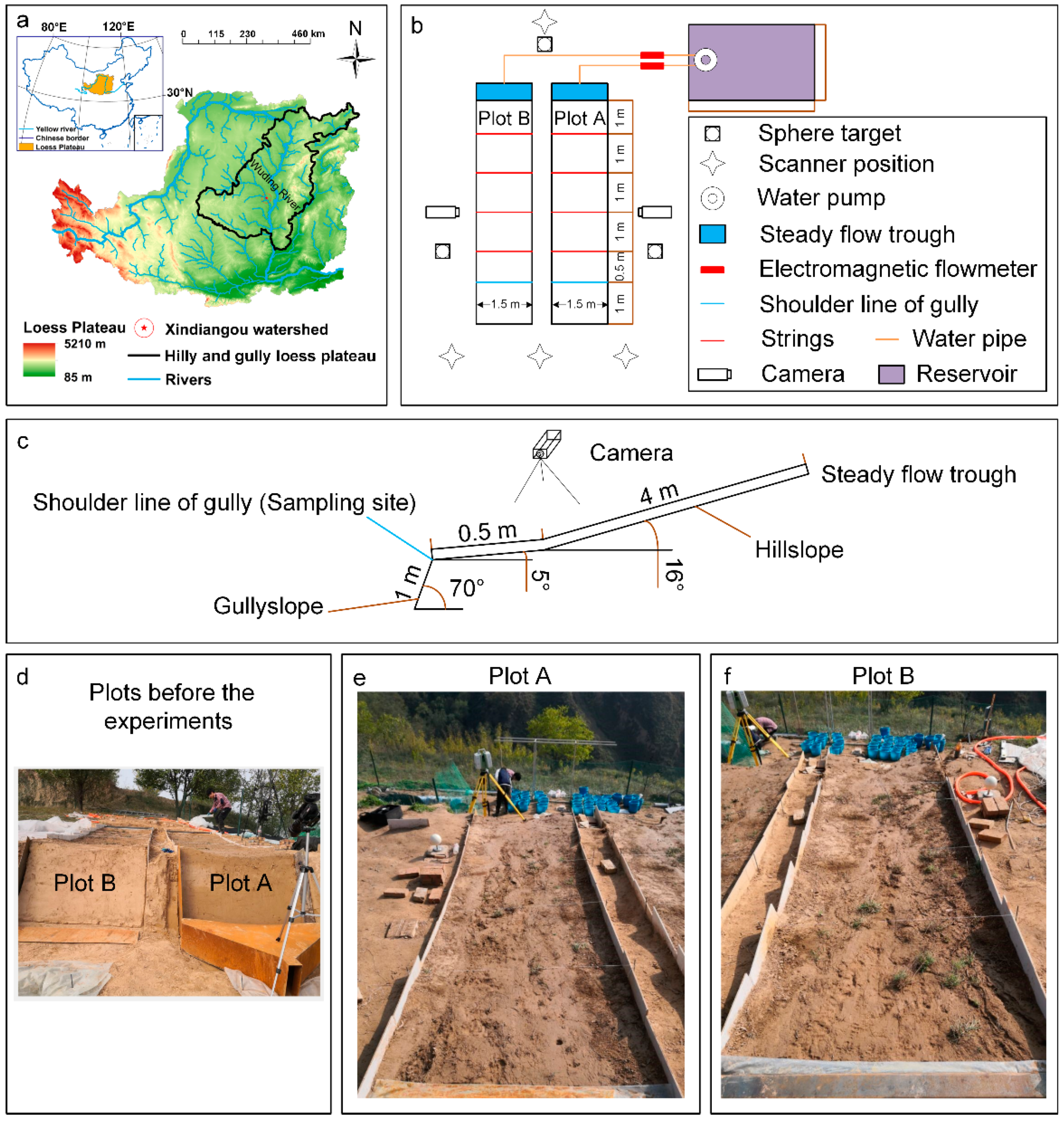
2.1. Study Site

The selected slopes are located in a small catchment (i.e., the Xindiangou catchment) of the hilly and gully loess plateau (Figure 1). Xindiangou is a tributary of the Wuding River, which is a first-order tributary of the Yellow River. The Xindiangou catchment covers 1.44 km², with an altitude ranging from 820 to 1180 m above sea level. The mean annual precipitation is 476 mm, of which 72.5% occurs between June and September in the form of short-duration intensive rainfall events.

The mean annual temperature is 10.2 °C, with maximum and minimum temperatures of 39.1 °C and −27.1 °C, respectively. The catchment is topographically complex and fragmented and features a typical geomorphology in the hilly and gully loess plateau. Gullies cover 46.8% of the catchment area, with a gully density of 7.26 km km⁻² [33]. The catchment is primarily covered by loess, which is loose and prone to erosion. Intensive rainfall and gravity act on the loose soil, particularly in sparsely vegetated areas, leading to serious erosion in the Xindiangou catchment.

2.2. Experimental Design and Establishment of Plots

Runoff scouring experiments and TLS were employed to study the hillslope erosion processes. In the hilly and gully loess plateau, hillslopes are an essential part of slope–gully systems (consisting of hillslopes and gully slopes), which are fundamental units for soil erosion and sediment production in the region. A study that ignores the relationship between the slope–gully system and its components cannot reflect the actual circumstances of erosion processes [34]. In this study, the erosion processes of hillslopes in the slope–gully system were investigated, to ensure that our experiments were capable of reproducing the actual erosion processes.

We investigated 20 typical slope–gully systems within and around the Xindiangou catchment. The baseline data showed that the slope gradients of the hillslopes were between 3° and 35°, while those of gully slopes were between 45° and 78°. Two slope–gully systems (named plots A and B, Figure 1) were established on a natural slope with a sharp slope break.

The upper part (i.e., above the break) was used to represent hillslopes with slope gradients of 3–17.5°, while the lower part (i.e., below the slope break) was used to represent gully slopes (slope gradient = 70°). The microtopography of hillslopes was slightly adapted to ensure a concentrated runoff flow at the bottom of the hillslopes, while the gully slopes were established by manually reshaping the slopes below the slope breaks to a 70-degree plane. These two plots were used to study the spatiotemporal patterns of the erosion processes on hillslopes.

According to the size of the selected slope, the length of the plots (slope–gully systems) was set to 5.5 m (a 4.5-m hillslope and 1-m gully slope) to ensure sufficient space for other experimental equipment (e.g., steady flow trough, TLS, and water pipes). The width of both plots was set to 1.5 m, which is comparable with other field experiments undertaken in the hilly and gully loess plateau.

Both plots were fenced with 60 cm (length) × 30 cm (height) tiles, with 20 cm buried and 10 cm remaining above ground. Before the experiments, the aboveground vegetation on the hillslopes was cut to a 5-cm height to facilitate clear observations of the geomorphology and runoff-erosion processes while at the same time allowing the remaining vegetation (5 cm) to maintain a position higher than the runoff depth such that the vegetation retained its function as a resistance to runoff.

A steady flow trough (150 cm × 30 cm × 50 cm) was installed at the upper end of the hillslopes to supply water flow. One 40-m³ water reservoir was established several meters away from the plots. An electromagnetic flowmeter was installed in the water pipes between the water reservoir and steady flow trough to control the flow discharge. Four strings, stretching across the hillslopes, were set up at 10 cm above the ground, at 1-m intervals. TLS was then used to scan the plots and produce point clouds, while three sphere targets were placed on concrete platforms around the plots for point cloud registration. A camera was placed 2 m above the plots to record the entire process of the experiments. To avoid any disturbance to the experiments and TLS scanning, the camera was installed to the side of the plots, as opposed to directly overhead.

To ensure that the flow discharge used in the experiment was consistent with the rainfall–runoff generating characteristics of the Xindiangou catchment, the flow discharge was calculated according to the algorithm (Equation (1)) developed by [35]:

$$F=\frac{W}{D}\cdot I\cdot A\cdot \cos \theta \cdot \partial$$

(1)

where F is the flow discharge, (L min⁻¹); W is the width of the plots (1.5 m); D is the width of the hillslopes, set to 5 m in terms of the topography in the Xindiangou catchment; I is the rainfall intensity (mm min⁻¹), set to 0.3–0.6 mm based on the historical precipitation of the Xindiangou catchment [36]; A is the drainage area, set to 300–400 m² for the Xindiangou catchment; θ is the slope gradient, set to 16.35°; and ∂ is the runoff coefficient, set to 0.324–0.568 with reference to the historical field plot measurements (excluding extreme measurements) in the Xindiangou catchment [36]. As a result, the calculated F ranged between 8.39 and 39.24 L min⁻¹. Finally, we set the flow discharge to 25 L min⁻¹, which represents a typical runoff flow discharge for the study site.

During the experiments, the concentrated runoff flow from hillslopes led to the development of gullies on the gully slopes and to the retreat of gully shoulder lines (approximately 0.4 m and 0.7 m in plots A and B, respectively, following the cessation of the 14 experiments) (Figure 2). The division of hillslopes and gully slopes changed along with the development of gullies, resulting in a dynamic hillslope area. In this case, the area below the top point of the gully shoulder line (yellow area in Figure 2) became the contributing area of gully erosion (i.e., gully slopes), while the other areas of the plots remained as hillslopes (brown area in Figure 2).

2.3. Data Collection and Processing

2.3.1. Collection of Sediment and Runoff

Fourteen runoff scouring experiments were carried out on plots A and B, respectively. Each of the experiments lasted for 30 min, which is similar to the duration of local rainfall events [36]. Measuring cylinders were employed to collect water samples once every 2 min at the top point of the gully shoulder line and its vicinity (Figure 2b), where the runoff flow from the hillslopes was concentrated.

The collected samples were then weighed using an electronic balance with an accuracy of 0.1 g. After the experiments, the samples were first allowed to settle, then put into alluvium boxes and oven-dried at 105 °C for 24 h. The dried samples were weighed again using an electronic balance. The sediment concentration was then calculated as the ratio of the sediment mass to the volume of clear runoff, and the runoff ratio was determined as the ratio between the volume of clear runoff and that of the muddy runoff sample.

During the experiments, the runoff depth at each of the strings was measured once every 2 min using a steel rule with 1-mm accuracy. A potassium permanganate solution was poured into the runoff flow at each string, and the movement of the potassium permanganate solution along with the runoff was recorded by the camera. After the experiments, the videos were transferred to photos using Freestudio software at 5-frame intervals. The runoff flow velocity was then determined through the distance and corresponding time duration derived from the photos.

The runoff width was determined using the Digimizer software based on the photos. The width, depth, and velocity measurements of the runoff flow measured at each of the strings were then averaged to produce the average runoff width, depth, and velocity for each interval. The muddy runoff discharge from the plots was then derived based on the average runoff width, depth, and velocity using Equation (2):

$$R_m=\frac{v_r\cdot w_r\cdot d_r\cdot t}{1000}$$

(2)

where R_m is the muddy runoff discharge (L), v_r is the average runoff velocity (m s⁻¹), w_r is the average runoff width (m), d_r is the average runoff depth (m), and t is the measurement interval (s). The runoff and sediment discharge were then determined based on the muddy runoff discharge, runoff ratio, and sediment concentration using Equations (3) and (4):

$$\begin{array}{l}{V}_{cr}=\frac{m_{mr}-m_s}{{\rho }_w}\cdot 1000\\ \\ {\zeta }_r=(\frac{V_{cr}}{V_{mr}})\cdot 100\%\\ \\ R=R_m\cdot {\zeta }_r\end{array}$$

(3)

where V_cr is the volume of clear water in the samples (L), m_mr is the mass of muddy runoff in samples (kg), m_s is the mass of sediment in the samples (kg), ρ_w is the density of water (1 × 10³ kg m⁻³), V_mr is the volume of muddy water in the samples (L), R is the runoff discharge (L), and ζ_r is the runoff ratio:

$$\begin{array}{l}S=R\cdot s_r\\ \\ s_r=m_s/V_{cr}\end{array}$$

(4)

where S is the sediment yield (kg) and s_r is the sediment concentration of runoff (kg L⁻¹).

2.3.2. Acquisition and Processing of LiDAR Point Clouds

• LiDAR point cloud acquisition

Prior to the first runoff scouring experiment, plots A and B were scanned by TLS to acquire the original terrain of the plots. During the experiments, the plots were repeatedly scanned after each of the 14 runoff scouring experiments. A Leica ScanStation C10 was employed, with a measurement range of up to 300 m, which can produce point clouds with millimeter-level accuracy if the parameters are properly adjusted. The positional accuracy, range accuracy, and target scanning accuracy reached 6, 4, and 2 mm, respectively, after an optimization of the parameters. The wavelength, maximum scanning velocity, and vertical and horizontal scanning angles were finally set to 532 nm, 5 × 10⁴ points per second, and 270° and 360°, respectively. The TLS was set up three to four times at the upper end of hillslopes and the bottom of gully slopes. The scanning position on the upper-slope area was mainly used to acquire point clouds for hillslopes, while those at the bottom of gully slopes not only provided additional point clouds for hillslopes and helped to avoid occlusions, but also facilitated the monitoring of the retreat of the gully shoulder lines and the dynamic changes of the hillslope area. The height of the scanner was set to 1.5–2.0 m above the ground. Achieving a scanning height of over 2.0 m was difficult, given the complex topography around the plots and the limits of our TLS system.

• Registration of LiDAR point clouds

After data acquisition, the point clouds of different scans were registered, using the Leica Cyclone software to form an integrated point cloud for each experiment based on the sphere targets around the plots (i.e., scan-to-scan registration). The integrated point clouds for different experiments were then co-registered using the Align tool of CloudCompare open source software, version 2.11 (i.e., scan-set to scan-set registration). Finally, the integrated point clouds were filtered using Terrasolid 2016 software to produce ground point clouds by manually selecting and clipping unnecessary points (e.g., tiles, and cotton threads) [37]. As a result, the final density of the ground points for plots A and B were 5.11 × 10⁵ and 5.05 × 10⁵ points m⁻², respectively.

• Derivation of volumetric changes and soil erosion mass

Elevation changes in the plots between experiments were detected based on the achieved point clouds to assess soil erosion across hillslopes. Commonly used methods for elevation change detection include the DEM of differences (DoD) [38,39,40,41], direct cloud-to-cloud comparison with closest point (C2C) [42] cloud-to-mesh distance (C2M) [43], and multiscale model to model cloud comparison (M3C2) [44]. DoD and C2M involve the generation of DEM or mesh via interpolation processes [40,42], which may bring about uncertainties in surface change detection. The C2C is simple and fast, but it is sensitive to the cloud’s roughness, outliers, and point density, and thus is better suited for rapid change detection on very dense point clouds rather than for accurate distance measurement [42]. M3C2 is able to overcome the drawbacks of DoD, C2M, and C2C by comparing point clouds directly without gridding or meshing and offers better accounting for changes in the point density and point cloud noise [44]. Therefore, we chose the M3C2 method for elevation change detection in our study.

The M3C2 algorithm is available in the CloudCompare software, and its essential parameters are the normal scale (D) and projection scale (d). For any given point k in the reference point cloud, D is the diameter of a modeled disk whose center is k. Points of a reference point cloud that fall within the disk are used by the algorithm to fit a plane, and the normal vector of that plane is calculated for point k. A cylinder with radius d is then defined, where the axis parallels the normal vector and passes through point k.

The cylinder intercepts the reference cloud and comparison cloud, resulting in two subsets of points I and J. After projecting these two subsets of points on the axis of the cylinder, the mean positions on the axis of each subset of points are defined as i and j. The length from i to j along the axis is the elevation change for point k (L). To optimize the calculations, parameter D is suggested to be 20–25 times that of the local roughness scale, while d should be smaller than D, and chosen to include a minimum of 20 scan points [44]. According to these guidelines, for this study, D and d were assigned the values of 2.5 and 2 cm, respectively.

Registration error is inevitable during the scan-to-scan and scan set-to-scan set registrations and may result in false change detections [42]. Thus, the level of detection (LoD) was employed to separate “true” and “false” changes [39]. In the M3C2 method, the LoD at the 95% confidence interval is derived based on registration errors and local roughness (Equation (5)):

$$LoD=\pm 1.96(registrationerror+\sqrt{\frac{{\sigma }_1{(d)}^2}{n_1}+\frac{{\sigma }_2{(d)}^2}{n_2}})$$

(5)

where the registration error refers to the M3C2 distance (L) for the three concrete platforms around the plots between two scan sets; σ₁(d)² and σ₂(d)² are calculated as the standard deviation of elevations of the subset of points (I, J) in the cylinder; and n₁ and n₂ are the number of subsets of points in the cylinder.

Once the distance measurements and LoD for each point were achieved, points with significant changes were used for volumetric change derivation. A new point cloud was then generated by assigning the M3C2 distance to each of the points with L over LoD and assigning zero to points with L less than LoD. The new point cloud was then gridded, and the z value of each grid was the average value of the points within the grid cell.

The volume of the grid cell equals the grid-cell size multiplied by the z value. The volumetric change of the whole plot was achieved by summing the volume of each grid cell, where negative volumes indicate erosion and positive values indicate deposition [16]. As mentioned above, the hillslope area reduced as gullies developed; therefore, the area of hillslopes used for topographic change estimation was the same as that resulting from the later conducted experiment.

The grid-cell size (resolution) affects the accuracy of the volumetric change calculations [45]. Therefore, in this study, we adopted different grid-cell sizes (1, 2, 5, 8, 10, 15, and 20 mm) to derive the volumetric changes. Two types of volumetric changes were calculated: consecutive volumetric changes (i.e., changes between the nth scan set and (n-1)th scan set) and cumulative volumetric changes (i.e., changes between different scan sets and the first scan sets describing the initial topography of the plots).

The soil bulk density was measured using the oven-drying method based on the samples collected from the upper, middle, and lower parts of the hillslopes (1.28 and 1.22 g cm⁻³ for hillslopes of plots A and B, respectively). The volumetric changes, derived based on different grid-cell sizes, were then converted to sediment mass based on the soil bulk density. The sediment masses corresponding to consecutive volumetric changes and cumulative volumetric changes refer to the calculated cumulative sediment yield and consecutive sediment yield, respectively. A comparison of the calculated sediment yield and measured sediment yield was conducted to evaluate the accuracy of TLS for the study of hillslope erosion processes.

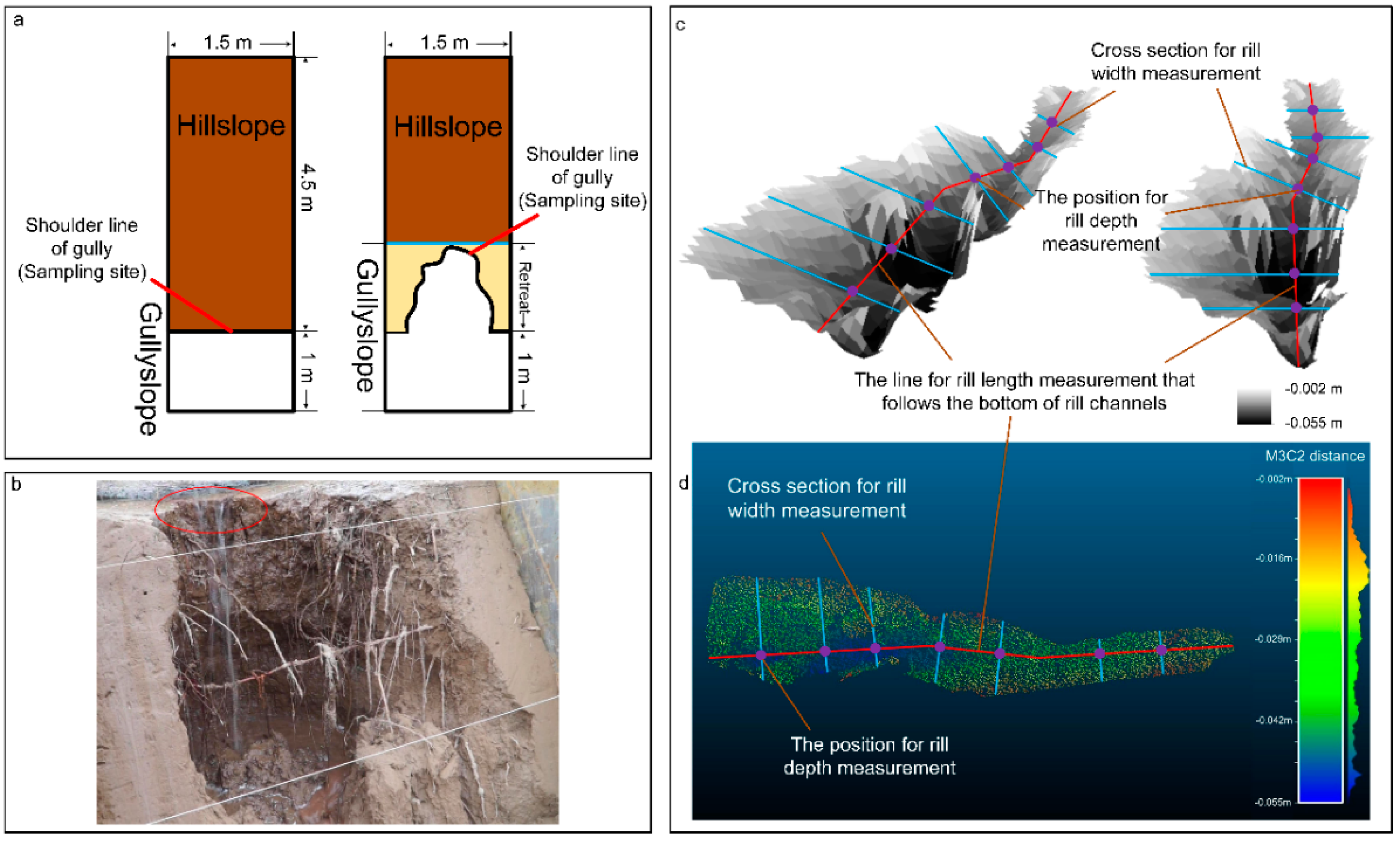
• Derivation of rill dimensions

Once the accuracy of the TLS point clouds was assessed, the rill dimension (width, length, and depth) was manually measured using the CloudCompare software based on the LoD-thresholded topographic change point clouds, with the aid of photos of the plots converted from videos.

The position of the rills was first roughly determined based on the photos of the plots. A 5-mm DEM was then generated from the topographic change point clouds for the area corresponding to the rough position of the rills. The exact extent of the rills was identified based on the DEM as the area with negative elevation values that featured a long-strip shape and approximately followed the direction of runoff (Figure 2c). Once the extent of rills has been determined, the topographic change point clouds for rills were extracted for the measurement of rill dimensions (Figure 2e).

A line following the bottom of rill channels was drawn for the rill length measurement. Cross-sections were set for the rill width measurement, and the distance between them was set to 3–8 cm according to the length and shape of rills. The rill depth was measured at the intersection points of the line and cross-sections. The rill length was derived as the length of the line, while the rill width and depth were calculated as the average value of the corresponding measurements at different positions. The measurements were undertaken after each of the runoff scouring experiments and then used to derive the average value and range of the width, length, and depth of the rills for each of the experiments.

3. Results

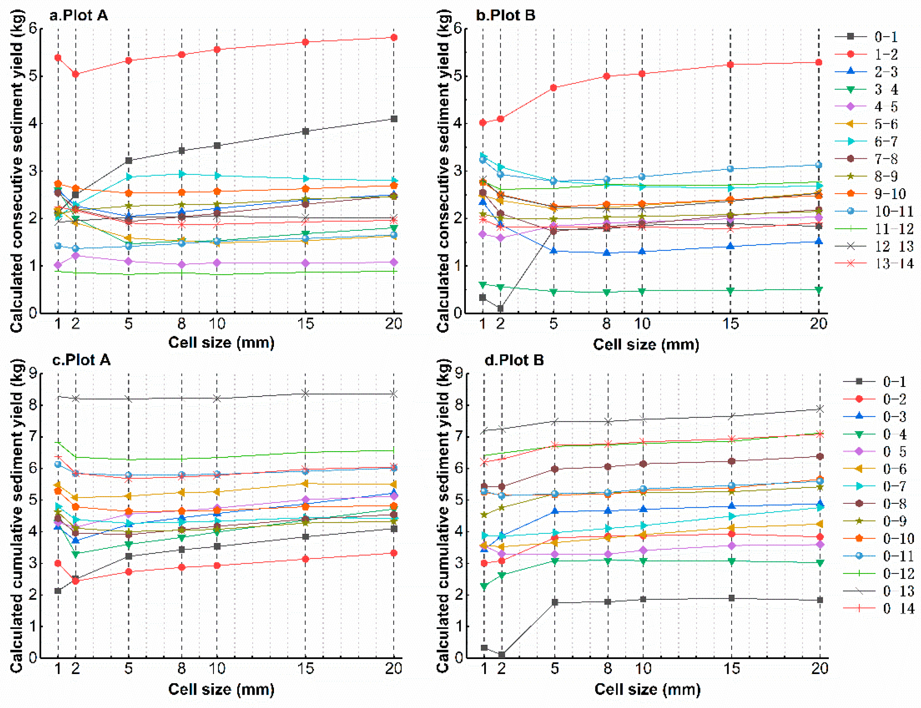
3.1. Accuracy of the Sediment Yield Derived using Terrestrial Laser Scanning

The TLS-derived (calculated) cumulative sediment yield and consecutive sediment yield (i.e., sediment yield for individual experiments) changed with the grid-cell sizes (Figure 3). The fluctuations in the calculated sediment yield decreased as the grid-cell size surpassed 5 mm, meaning that a grid-cell size of over 5 mm provided a more stable result. Therefore, we assessed the accuracy of the TLS-derived sediment yield by comparing the calculated sediment yields for grid-cell sizes of more than 5 mm with the measured values.

Under a 5–20 mm grid-cell size, poor agreement was found between the calculated and measured consecutive sediment yields of the 14 experiments (R² < 0.5) (

Table 1. The magnitude of absolute errors and relative errors for the calculated sediment yields of hillslopes and quality of the linear regression between the calculated and measured sediment yields for the 14 experiments under the 5 mm–20 mm grid-cell size.

	Plot	Cell Size (mm)	Magnitude of Absolute Errors (kg)			Magnitude of Relative Errors (%)			Linear Relation
			Max	Min	Mean	Max	Min	Mean	R2	p
Consecutive sediment yield	A	5	4.76	0.56	1.67	4705.44	80.21	784.12	0.11	0.245
		8	4.88	0.60	1.72	4905.49	87.61	805.28	0.13	0.211
		10	4.99	0.55	1.74	5070.74	88.55	820.23	0.14	0.196
		15	5.15	0.60	1.83	5266.4	106.65	853.71	0.16	0.150
		20	5.25	0.62	1.91	5518.67	121.92	888.86	0.19	0.123
	B	5	3.81	0.28	1.73	1180.65	153.15	466.21	0.47	0.006
		8	4.06	0.27	1.76	1204.23	145.84	473.67	0.46	0.007
		10	4.11	0.29	1.79	1216.81	160.46	480.71	0.47	0.007
		15	4.30	0.30	1.86	1242.75	165.11	502.07	0.45	0.009
		20	4.35	0.32	1.94	1286.78	175.74	524.83	0.44	0.010
Cumulative sediment yield	A	5	1.79	0.004	0.87	124.49	0.06	25.02	0.61	<0.001
		8	2.00	0.02	0.89	139.22	0.33	26.65	0.58	0.001
		10	2.10	0.06	0.90	146.26	0.94	27.54	0.58	0.002
		15	2.40	0.11	0.98	167.59	1.80	31.19	0.55	0.003
		20	2.67	0.01	1.04	185.79	0.12	34.32	0.50	0.005
	B	5	2.78	0.12	1.26	180.06	2.34	56.82	0.82	<0.001
		8	2.80	0.16	1.30	183.55	3.06	58.48	0.82	<0.001
		10	2.85	0.27	1.37	195.96	5.39	61.23	0.83	<0.001
		15	2.95	0.38	1.47	200.81	7.46	64.64	0.83	<0.001
		20	3.03	0.51	1.59	192.27	10.07	66.73	0.84	<0.001

). The calculated consecutive sediment yields were always higher than the measured values, with the average values of the former being four to eight times those of the latter. However, the calculated cumulative sediment yields were found to correspond well with measured values. Significant linear relations were found between the calculated and measured values, with R² values greater than 0.50 and 0.82 for plots A and B, respectively.

The calculated cumulative sediment yield was always higher than the measured values for plot B, and sometimes lower than the measured values in plot A (Figure 4a,b), with the magnitude of relative errors being no more than 200%. The magnitudes of the absolute and relative errors of the calculated consecutive sediment yields were generally higher than those of the calculated cumulative sediment yields (Figure 4c,d), while the R² corresponding to the consecutive sediment yield was lower than that corresponding to the cumulative sediment yield.

As the grid-cell size decreased, the magnitude of absolute and relative errors of the calculated cumulative sediment yield also decreased, and the R² for plot A increased, while the R² for plot B slightly decreased (Table 1). The most accurate calculated sediment yields were achieved at the 5-mm grid-cell size, with the mean absolute/relative error being 0.87 kg/25.02 % and 1.26 kg/56.82 %, and R² being 0.61 (p < 0.001) and 0.82 (p < 0.001) for hillslopes of plots A and B, respectively (Table 1, Figure 4a,b). Hence, the cumulative terrain change from the original topography was employed to study the spatiotemporal pattern of erosion processes.

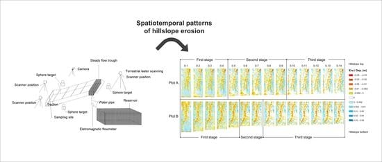
3.2. Spatiotemporal Patterns of Erosion Processes

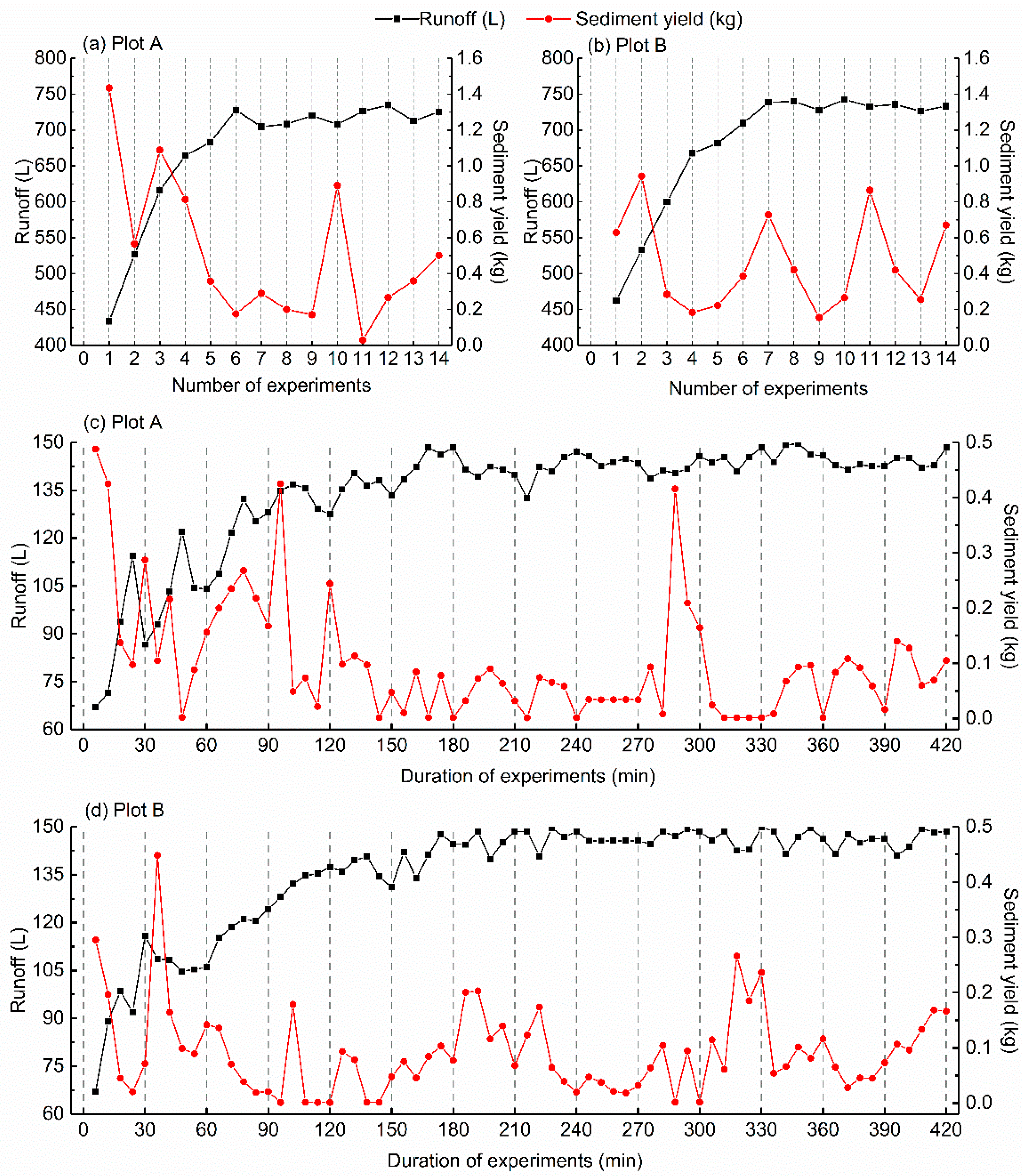
3.2.1. Measured Runoff and Sediment Discharge from Hillslopes

During the 14 experiments, the hillslope of plot A produced 9390.9 L of runoff and 7.1 kg of sediment, respectively, with the runoff and sediment yield for the individual experiments ranging from 433.49–734.68 L and 0.03–1.43 kg, respectively. The hillslope of plot B produced 9530.5 L of runoff and 6.4 kg of sediment, with the runoff and sediment yield for the individual experiments ranging from 462.44–742.53 L and 0.16–0.94 kg, respectively. The runoff production from both hillslopes increased during the first five experiments and became stable after the sixth experiment.

The sediment yield generally followed a decreasing trend during the first five experiments, with the highest sediment yield occurring in the first and second experiments, respectively. However, it fluctuated considerably during the sixth to the fourteenth experiments, over which several peaking sediment yields from hillslopes occurred, including the tenth experiment for plot A (0.89 kg) and the seventh and eleventh experiments of plot B (0.73 kg and 0.86 kg).

The runoff and sediment yield corresponded relatively well during the first five experiments, with the runoff production increasing and sediment yield generally decreasing (Figure 5). However, the sediment yield fluctuated considerably in the context of relatively stable runoff production during the sixth to the fourteenth experiments, weakening the connection between runoff and sediment yield. As a result, the relationships between runoff and sediment yield were not strong. The R² of the linear regression between the inter-experiment runoff and sediment (i.e., runoff and sediment yield for each experiment) was 0.57 (p = 0.002) and 0.08 (p = 0.321), respectively, and that of the intra-experiment runoff and sediment (i.e., runoff and sediment yield during every 6 min) was 0.37 (p < 0.001) and 0.06 (p = 0.035).

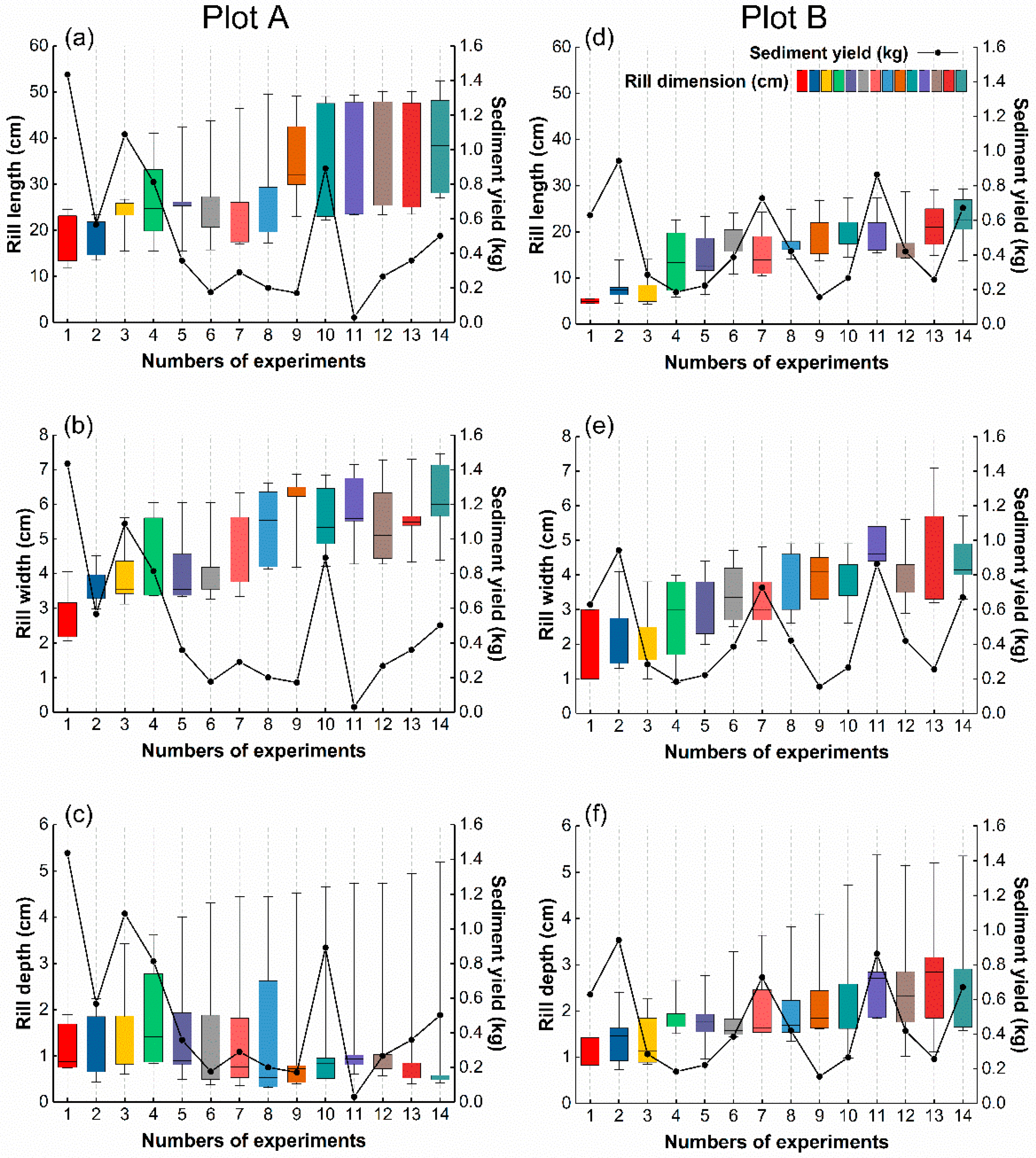
3.2.2. Spatiotemporal Development of Hillslope Erosion Processes

During the experiments, the development of the hillslope erosion processes experienced three major stages. The area with erosion/deposition decreased and the intensity of the erosion (the depth of soil removed by erosion) increased toward the end of the experiments (Figure 6). The first stage corresponded to the first four/five experiments in plot A/plot B. During this stage, the erosion processes developed relatively quickly, and resulted in a widespread distribution of erosion and deposition across the hillslopes. The erosion was particularly distributed on the upper to middle parts of hillslopes, while the deposition was more prevalent in the lower parts of the hillslopes.

The second stage spanned from the fifth/sixth to the ninth/seventh experiment in plot A/plot B. A sharp increase in area, with insignificant topographic changes, led to a considerable shrinkage in the area with deposition. The third stage included the tenth/eighth to the fourteenth experiment in plot A/plot B. The spatial pattern of erosion and deposition tended to be stable. The occurrence of erosion became more concentrated than in the first and second stages, and the area of intensive erosion (elevation decrease > 0.02 m) increased. In terms of the TLS results, the cumulative hillslope erosion of plots A and B was 8.58–14.02 kg and 7.00–14.47 kg, and the cumulative sediment deposition was 5.36–7.12 kg and 3.91–11.83 kg, respectively.

In plot A, the rills were mainly concentrated on the right side and almost continuously stretched from the top to the bottom of the hillslope, although several discontinuities occurred (Figure 6). In plot B, the rills were dispersed on the upper part while concentrated on the middle part of the hillslope to form a major channel that was wider and deeper than all other channels. During the experiments, the length and width of the rills increased over time, and those of plot A were higher than those of plot B (Figure 7). The rill depth of plot A did not change, while that of plot B increased throughout the experiments. Overall, the rills of plot B were deeper than those of plot A, particularly after the ninth experiment, while they were narrower and shorter than the rills of plot A.

In addition, the peak sediment yield from the hillslopes corresponded well to the changes in rill width and length during the same or last experiment (Figure 7). For example, the peaking sediment yield and rapid increase in rill length occurred simultaneously in the third experiment of plot A and the second experiment of plot B; the peak sediment yield in the tenth experiment of plot A and the seventh experiment of plot B occurred after a rapid increase in the rill length during the last experiment; both the peak sediment yield and a rapid increase in the rill width occurred in the eleventh experiment of plot B.

In terms of the relationships between the development of rills and the erosion–transport–deposition processes, significant linear relationships were scarce between calculated cumulative deposition and rill dimensions for hillslopes in plots A and B (

Table 2. Linear regression between the dimensions (maximum, minimum, average length, width, and depth) of rills and the cumulative soil erosion, deposition, and sediment yield from the hillslopes of plots A and B.

Plot	Rill Dimension (cm)	TLS-Derived Erosion (kg)			TLS-Derived Deposition (kg)			TLS-Derived Sediment Yield (kg)			Measured Sediment Yield (kg)
		Slope	R2	p	Slope	R2	p	Slope	R2	p	Slope	R2	p
A	Max. rill length	0.08	0.32	0.037 *	−0.01	0.03	0.574	0.09	0.39	0.016 *	0.15	0.87	<0.001 **
	Min. rill length	0.18	0.36	0.023 *	−0.03	0.07	0.350	0.21	0.50	0.005 *	0.34	0.86	<0.001 **
	Ave. rill length	0.13	0.44	0.010 *	−0.02	0.05	0.464	0.15	0.56	0.002 *	0.23	0.90	<0.001 **
	Max. rill width	0.96	0.48	0.006 *	−0.05	0.01	0.727	1.01	0.54	0.003 *	1.62	0.96	<0.001 **
	Min. rill width	1.15	0.32	0.035 *	−0.14	0.03	0.550	1.29	0.40	0.015 *	2.26	0.86	<0.001 **
	Ave. rill width	0.73	0.27	0.046 *	−0.06	0.01	0.695	0.79	0.32	0.034 *	1.51	0.83	<0.001 **
	Max. rill depth	0.99	0.47	0.007 **	−0.05	0.01	0.755	1.04	0.53	0.003 *	1.66	0.93	<0.001 **
	Min. rill depth	−0.54	0.003	0.855	1.10	0.08	0.316	−1.64	0.03	0.573	−3.82	0.10	0.266
	Ave. rill depth	1.69	0.09	0.303	1.19	0.30	0.042 *	0.50	0.01	0.766	1.34	0.04	0.500
B	Max. rill length	0.19	0.36	0.023 *	−0.11	0.20	0.107	0.17	0.54	0.003 *	0.22	0.74	<0.001 **
	Min. rill length	0.42	0.67	<0.001 **	−0.01	0.07	0.360	0.29	0.63	<0.001 **	0.36	0.80	<0.001 **
	Ave. rill length	0.27	0.45	0.008 *	−0.13	0.20	0.107	0.21	0.54	0.003 *	0.28	0.80	<0.001 **
	Max. rill width	2.08	0.60	0.001 *	−0.49	0.06	0.397	1.74	0.81	<0.001 **	1.97	0.87	<0.001 **
	Min. rill width	1.53	0.55	0.003 *	−0.36	0.05	0.426	1.02	0.47	0.007 *	1.37	0.72	<0.001 **
	Ave. rill width	1.93	0.58	0.001 *	−0.66	0.12	0.217	1.35	0.55	0.002 *	1.8	0.84	<0.001 **
	Max. rill depth	1.32	0.60	0.001 *	−0.33	0.07	0.370	1.06	0.74	<0.001 **	1.31	0.96	<0.001 **
	Min. rill depth	0.71	0.02	0.674	−2.06	0.23	0.079	0.61	0.02	0.615	1.82	0.16	0.150
	Ave. rill depth	2.77	0.51	0.004 *	−1.02	0.13	0.214	2.24	0.64	<0.001 **	2.88	0.90	<0.001 **

* indicates significance at p < 0.05, ** indicates significance at p < 0.001.

).

In plot A, the rill dimensions (except for the minimum and average rill depths) were significantly positively correlated with the calculated cumulative hillslope erosion, calculated cumulative hillslope sediment yield, and measured cumulative hillslope sediment yield. The increase rate (i.e., slopes of the linear regression) of the cumulative erosion and sediment yield with rill dimensions followed the order of minimum rill width > maximum rill depth > maximum rill width > average rill width > minimum rill length > average rill length > maximum rill length.

Similarly, in plot B, the rill dimensions (except for the minimum rill depth) were also significantly positively correlated with the calculated cumulative hillslope erosion, calculated cumulative hillslope sediment yield, and measured cumulative hillslope sediment yield. The rate of increase in the erosion and sediment yield with rill dimensions followed the order of average rill depth > maximum rill width > average rill width > minimum rill width > maximum rill depth > minimum rill length > average rill length > maximum rill length.

Overall, the development of the rills did not significantly impact the cumulative deposition, while they did impact the erosion and sediment yield from hillslopes. The development of the rill depth and rill width had a higher impact compared with that of the rill length on the cumulative erosion and sediment yield from hillslopes.

4. Discussion

4.1. The Design of the Study

Previous studies investigating hillslope erosion using TLS were typically conducted on plots established using backfill soils [16,46,47]. The soil properties (e.g., soil structure) on backfill plots are different from those of natural soil. This means that soil erosion processes on backfill plots are not able to fully represent those on a field hillslope, limiting the applicability of findings to field hillslopes.

In the study, we investigated hillslope erosion based on in-situ scouring experiments and TLS. The slope-gully system chosen in our study was selected based on a survey of natural slope-gully systems. The released runoff discharge was determined in terms of the local rainfall intensity. According to the historical measurements of field runoff plots from 1954 to 1963 issued by the Yellow River Conservancy Commission [36], the sediment yields from hillslopes in the Xindiangou catchment were 2.9 × 10⁻⁵ to 1.9 × 10⁻¹ kg min⁻¹ m⁻², which are comparable with our results (1.8 × 10⁻⁴ to 0.8 × 10⁻¹ kg min⁻¹ m⁻²). This demonstrated that our experiment is capable of reflecting the actual erosion processes on hillslopes, providing a direct reference to the monitoring and study of the hillslope erosion processes. Previous studies have employed TLS to monitor the erosion processes in the field hillslopes [14,28,29], through directly applying TLS without evaluating its accuracy in the application environment. We found that the accuracy of the TLS-derived cumulative sediment yield was higher than that of the TLS-derived consecutive sediment yield, which was rather low. This demonstrated that TLS is suitable for monitoring long-term/relatively heavy hillslope erosion, which normally leads to a higher topographic change, but is incapable of monitoring the hillslope erosion induced by a regular rainfall event. However, our results may not be transferable to other soil systems or environment settings, as the development of erosion processes is heavily influenced by soil properties and other environmental conditions [48,49]. Therefore, we suggested that the accuracy of TLS should be assessed in the application environment before TLS is applied in erosion monitoring in the future.

4.2. Uncertainty in TLS Results

Our results are subject to uncertainties (inaccuracies), which could be explained by the following four aspects.

Firstly, we found that the calculated cumulative sediment yield was more accurate than the calculated consecutive sediment yield. In our study, the relative errors of the TLS-derived consecutive sediment yield at the 5-mm grid-cell size ranged between 80.21% and 4705.44%. These values were considerably higher than those experiments with higher sediment yields. For example, Li et al. [16] found that the average relative errors for TLS-derived consecutive sediment yields were 25.9% and 9.1% based on rainfall simulations that produced 40–60 kg of sediment. Based on indoor rainfall simulations, Zhang et al. [46] and Xiao et al. [47] found that the relative errors for TLS-derived consecutive sediment yield were 1.1–5.1% for sediment yields of 112.84–1143.19 kg, and 0.9–9.3% for sediment yields of 18.95–38.69 kg. The above difference in accuracy implies that the lower erosion rates in our study, which resulted in a smaller elevation change, may partly account for the uncertainty in our results.

Secondly, in the study hillslopes were considered as part of slope–gully systems during the investigation of the erosion processes. Although this reflected the actual field processes (i.e., the relationship between the slope–gully system and its components), the resulting changing hillslope area inevitably increased the uncertainty of our findings. Water sampling was undertaken every 2 min, while the TLS scanning was only conducted before and after each experiment (i.e., 30 min intervals). This means that water sampling results could capture the soil erosion produced on the hillslope area that collapsed during the experiments, while the TLS scanning could not. This weakened the relationship between the measured and TLS-derived sediment yield. Thus, a better relationship would be expected between the measured and TLS-derived sediment yield if this limitation could be addressed.

Thirdly, in our study, the scanning position was concentrated at the upper end of hillslopes and the bottom of the gully slopes, ensuring a relatively good balance between the monitoring of hillslope and the retreat of the gully shoulder lines. However, no scans were set on the sides of plots, which may have added uncertainty to our results [16]. The height of the scanners (1.5–2.0 m) at the bottom of gully slopes was offset by the vertical height of the gully slopes (~0.94 m), leading to a relatively small angle between the laser pulse and hillslope, thereby adding uncertainty to our results [28,50]. Therefore, our results may not represent the highest accuracy of field erosion monitoring based on TLS. Further studies should thus be undertaken to examine the accuracy of field erosion monitoring results under different combinations of scanning positions and heights.

Lastly, the M3C2 method was employed to derive the elevation change, avoiding the interpolation of the point cloud and thus the error caused by the interpolation. However, the normal orientation estimation using a plane surface may not be suitable for tracking high-frequency changes in a topographically complex area (e.g., rill walls) [44]. Further work should thus be done to improve the estimation of normal orientation, making the M3C2 method more robust for topographic change detection for areas with complex topography. In addition, the TLS-derived sediment yield varied with the grid-cell size chosen for volumetric change calculation [16]. In our study, we have assessed the calculated sediment yields for different grid-cell sizes and selected the cell size (5 mm) associated with the more accurate calculated sediment yield. However, the grid-cell sizes we chose were still limited. This means that the 5-mm cell size may not be the best choice. Therefore, more efforts can be made to further investigate the impact of grid-cell size on the TLS-derived sediment yield.

4.3. Spatiotemporal Patterns of the Soil Erosion Processes

We found that the development of hillslope erosion consisted of three major stages, which included a rapid increase (first stage), a sharp decrease (second stage), and a stable distribution (third stage) of areas with erosion/deposition. During the first stage, erosion mainly occurred on the upper-middle part of the hillslopes, while deposition was more prevalent on the lower part of the hillslopes. This is consistent with the findings of previous field tracer studies, such as those conducted in northeastern China [51,52] and the southern Central Andes [53]. The phenomenon may be attributed to the fact that the slope gradient of the upper-middle part of the hillslopes is higher than that of the lower part (Figure 1), which facilitates the development of erosion and deposition on the respective parts. In addition, a sharp increase in the area without erosion/deposition in the second stage is possibly attributable to the sheet erosion that led to a slight decrease of elevation in the area with deposition during the first stage. A stable distribution of erosion and deposition may be a result of the development of rills, which led to a concentrated flow and thus reduced the sheet erosion on hillslopes.

In our experiments, the sediment yield from the hillslopes fluctuated considerably, even when the runoff production was stable, leading to a weak relationship between the runoff and sediment yield. The evolution of the rills was found to correspond well with the sediment yield peaks. This may be because the development of rills (e.g., the collapse of rill walls) provided a large number of erodible materials that can be rapidly transported out of hillslopes through concentrated rill flow. That is to say, the evolution of rills can immediately increase the sediment yield, leading to a weakened connection between runoff and sediment yield. In addition, the spatiotemporal development of erosion processes was different between the hillslopes of plots A and B, possibly because of the difference in the runoff path driven by microtopography, and the difference in erosion resistance resulting from the heterogeneity of soil properties and vegetation.

We also found that the development of rills significantly impacted the cumulative erosion and sediment yield rather than the cumulative deposition from hillslopes, with the impact strength of the rill width and rill depth being apparently higher than the impact strength of the rill length. Previous studies have found that the development of rills largely enhanced the sediment concentration and sediment yield from hillslopes [19,20], confirming the importance of rills for sediment yield from hillslopes [54,55]. However, few studies investigated the impact of rill dimension on the erosion–transport–deposition process and were, thus, limited to a process-based understanding of rill development and its contribution to hillslope erosion.

4.4. Implications

Our results have research and practical implications. For future research, our study provided a reliable experiment scheme for field hillslope erosion monitoring and research. The scheme is transferrable to other regions with similar soil erosion conditions to the hilly and gully loess plateau, where rainfall and runoff flow are the major erosive agents [53,56]. However, care should be taken when this scheme is applied to other erosion conditions, where the hillslope erosion is driven by different erosive agents. For example, in northeastern China, the erodible materials on hillslopes produced by the freeze–thaw cycles may lead to an elevation increase and thus bring about difficulties regarding the separation of erosion and deposition based on the TLS data. Additionally, a high-resolution study of field hillslope erosion processes is undoubtedly beneficial for the development of process-based hillslope erosion models [21,22].

With regard to the control of hillslope erosion, we demonstrated that the development of hillslope erosion experienced three stages with different characteristics. This means that the priorities for erosion control are not the same at different erosion stages. For example, attention should be paid to sheet erosion during the early stage of hillslope erosion development, while rills should be the focus at the later stage of erosion development. We found that the impact strength of the rill width and rill depth on hillslope erosion was much higher than the impact strength of the rill length. This suggests that the prevention of the widening and deepening of rills is likely a more effective method for hillslope erosion control than controlling the length of rills.

5. Conclusions

In this study, fourteen runoff scouring experiments were conducted on two neighboring plots established on the field slopes of the hilly and gully loess plateau in China. TLS was employed to investigate the soil erosion processes across the plots during the experiments, and the M3C2 method was adopted to derive the elevation change from point clouds.

The results demonstrated that the accuracy of the TLS-derived cumulative sediment yield from hillslopes of the two plots was apparently higher than that of TLS-derived consecutive sediment yield. The magnitude of absolute error for the calculated consecutive sediment yield was 1.67 kg (0.56–4.76 kg) and 1.73 kg (0.28–3.81 kg), and that for the calculated cumulative sediment yield was 0.87 kg (0.004–1.76 kg) and 1.26 kg (0.12–2.78 kg).

The magnitude of relative error for the calculated cumulative sediment yield from hillslopes of the two plots was 25.02% (0.06–124.49%) and 56.82% (2.34–180.06%), and the R² values of the linear relationships between the calculated and measured cumulative sediment yield were 0.61 (p < 0.001) and 0.82 (p < 0.001), respectively, when a grid-cell size of 5 mm was chosen to convert the M3C2-derived elevation change to volumetric change.

The sediment yield from the hillslopes was subject to fluctuations even when the runoff production became stable, leading to a weak relationship (the inter-experiment R² values were 0.57 (p = 0.002) and 0.08 (p = 0.321), while the intra-experiment R² values were 0.37 (p < 0.001) and 0.06 (p < 0.035) for hillslopes of the two plots) between runoff and sediment yield.

The TLS scanning results showed that the development of hillslope erosion underwent three major stages, which included a rapid increase and widespread distribution, a sharp decrease, and a stable distribution of area with erosion/deposition. The development of rills impacted the cumulative erosion and sediment yield rather than the cumulative deposition, with the impact strength of the rill depth and rill width development being higher than the impact strength of the rill length. The peak sediment yield corresponded well with the evolution of rills and partly accounted for the weak relationship between runoff and sediment yield from the hillslopes.

References

1. Borrelli, P.; Robinson, D.A.; Fleischer, L.R.; Lugato, E.; Ballabio, C.; Alewell, C.; Meusburger, K.; Modugno, S.; Schütt, B.; Ferro, V.; et al. An assessment of the global impact of 21st century land use change on soil erosion. Nat. Commun. 2017, 8, 2013. [Google Scholar] [CrossRef] [Green Version]
2. Borrelli, P.; Robinson, D.A.; Panagos, P.; Lugato, E.; Yang, J.E.; Alewell, C.; Wuepper, D.; Montanarella, L.; Ballabio, C. Land use and climate change impacts on global soil erosion by water (2015–2070). Proc. Natl. Acad. Sci. USA 2020, 117, 21994–22001. [Google Scholar] [CrossRef] [PubMed]
3. De Vries, F.T.; Liiri, M.E.; Bjornlund, L.; Bowker, M.A.; Christensen, S.; Setala, H.; Bardgett, R.D. Land use alters the resistance and resilience of soil food webs to drought. Nat. Clim. Chang. 2012, 2, 276–280. [Google Scholar] [CrossRef]
4. Rodrigo-Comino, J.; Terol, E.; Mora, G.; Giménez-Morera, A.; Cerdà, A. Vicia sativa Roth. can reduce soil and water losses in recently planted vineyards (Vitis vinifera L.). Earth Syst. Environ. 2020, 4, 827–842. [Google Scholar] [CrossRef]
5. Tsunekawa, A.; Liu, G.; Yamanaka, N.; Du, S. Restoration and Development of the Degraded Loess Plateau, China; Springer: Tokyo, Japan, 2014; pp. 507–508. [Google Scholar]
6. Clarke, M.L.; Rendell, H.M. The impact of the farming practice of remodelling hillslope topography on badland morphology and soil erosion processes. Catena 2000, 40, 229–250. [Google Scholar] [CrossRef]
7. Hales, T.; Scharer, K.; Wooten, R. Southern Appalachian hillslope erosion rates measured by soil and detrital radiocarbon in hollows. Geomorphology 2012, 138, 121–129. [Google Scholar] [CrossRef]
8. Guo, D.W.; Yu, B.F.; Fu, X.D.; Li, T.J. Improved Hillslope Erosion Module for the Digital Yellow-River Model. J. Hydrol. Eng. 2014, 20, 1–11. [Google Scholar] [CrossRef]
9. Yang, X. State and trends of hillslope erosion across New South Wales, Australia. Catena 2020, 186, 104361. [Google Scholar] [CrossRef]
10. Zhang, L.T.; Gao, Z.L.; Li, Z.B.; Tian, H.W. Downslope runoff and erosion response of typical engineered landform to variable inflow rate patterns from upslope. Nat. Hazards 2016, 80, 775–796. [Google Scholar] [CrossRef]
11. Xu, X.; Zheng, F.; Wilson, G.V.; Zhang, X.C.; Qin, C.; He, X. Quantification of upslope and lateral inflow impacts on runoff discharge and soil loss in ephemeral gully systems under laboratory conditions. J. Hydrol. 2019, 579, 124174. [Google Scholar] [CrossRef]
12. Xu, J.X. Erosion caused by hyperconcentrated flow on the Loess Plateau of China. Catena 1999, 36, 1–19. [Google Scholar]
13. Van Maren, D.S.; Winterwerp, J.C.; Wu, B.S.; Zhou, J.J. Modelling hyperconcentrated flow in the Yellow River. Earth Surf. Process. Landf. 2009, 34, 596–612. [Google Scholar] [CrossRef]
14. Neugirg, F.; Kaiser, A.; Huber, A.; Heckmann, T.; Schindewolf, M.; Schmidt, J.; Becht, M.; Haas, F. Using terrestrial LiDAR data to analyse morphodynamics on steep unvegetated slopes driven by different geomorphic processes. Catena 2016, 142, 269–280. [Google Scholar] [CrossRef]
15. Nouwakpo, S.K.; Weltz, M.A.; McGwire, K. Assessing the performance of structure-from-motion photogrammetry and terrestrial LiDAR for reconstructing soil surface microtopography of naturally vegetated plots. Earth Surf. Process. Landf. 2016, 41, 308–322. [Google Scholar] [CrossRef]
16. Li, L.; Nearing, M.A.; Nichols, M.H.; Polyakov, V.O.; Cavanaugh, M.L. Using terrestrial LiDAR to measure water erosion on stony plots under simulated rainfall. Earth Surf. Process Landf. 2020, 45, 484–495. [Google Scholar] [CrossRef]
17. Wang, P.; Jin, X.; Li, S.D. Application of Handheld 3D Scanner in Quantitative Study of Slope Soil Erosion. IOP Conf. Ser. Earth Environ. Sci. 2018, 170, 022178. [Google Scholar] [CrossRef]
18. Wirtz, S.; Seeger, M.; Ries, J.B. Field experiments for understanding and quantification of rill erosion processes. Catena 2012, 91, 21–34. [Google Scholar] [CrossRef]
19. Qin, C.; Zheng, F.L.; Xu, X.M.; Wu, H.Y.; Shen, H.O. A laboratory study on rill network development and morphological characteristics on loessial hillslope. J. Soils Sedim. 2018, 18, 1679–1690. [Google Scholar] [CrossRef]
20. Michael, C.S.; Rorke, B.B. Hydraulic conditions for rill incision under simulated rainfall: A laboratory experiment. Earth Surf. Process. Landf. 1992, 17, 127–146. [Google Scholar]
21. Nearing, M.A.; Foster, G.R.; Lane, L.J.; Finkner, S.C. A process-based soil erosion model for USDA-Water Erosion Prediction Project technology. Trans. ASAE 1989, 32, 1587–1593. [Google Scholar] [CrossRef]
22. Hessel, R. Consequences of hyperconcentrated flow for process-based soil erosion modelling on the Chinese Loess Plateau. Earth Surf. Process. Landf. 2006, 31, 1100–1114. [Google Scholar] [CrossRef]
23. Yang, X.; Yu, B.; Zhu, Q. Climate change impacts on rainfall erosivity and hillslope erosion in NSW. In Proceedings of the 21st International Congress on Modelling and Simulation, Gold Coarst, Australia, 29 November–4 December 2015. [Google Scholar]
24. Evans, M.; Lindsay, J. High resolution quantification of gully erosion in upland peatlands at the landscape scale. Earth Surf. Process. Landf. 2010, 35, 876–886. [Google Scholar] [CrossRef]
25. Chico, G.; Clutterbuck, B.; Midgley, N.G.; Labadz, J. Application of terrestrial laser scanning to quantify surface changes in restored and degraded blanket bogs. Mires Peat 2019, 24, 1–24. [Google Scholar]
26. Goodwin, N.R.; Armston, J.D.; Muir, J.; Stiller, I. Monitoring gully change: A comparison of airborne and terrestrial laser scanning using a case study from Aratula, Queensland. Geomorphology 2017, 282, 195–208. [Google Scholar] [CrossRef]
27. Telling, J.; Lyda, A.; Hartzell, P.; Glennie, C. Review of Earth science research using terrestrial laser scanning. Earth Sci. Rev. 2017, 169, 35–68. [Google Scholar] [CrossRef] [Green Version]
28. Usmanov, B.; Yermolaev, O.; Gafurov, A. Estimates of slope erosion intensity utilizing terrestrial laser scanning. Proc. Int. Assoc. Hydrol. Sci. 2015, 367, 59–65. [Google Scholar] [CrossRef]
29. Eltner, A.; Mulsow, C.; Maas, H. Quantitative measurement of soil erosion from TLS and UAV data. Int. Arch. Photogramm. Remote Sens. Spat. Inf. Sci. 2013, 40, 4–6. [Google Scholar] [CrossRef] [Green Version]
30. Eltner, A.; Maas, H.; Faust, D. Soil micro-topography change detection at hillslopes in fragile Mediterranean landscapes. Geoderma 2018, 313, 217–232. [Google Scholar] [CrossRef]
31. Zhao, G.; Mu, X.; Wen, Z.; Wang, F.; Gao, P. Soil erosion, conservation, and eco-environment changes in the loess plateau of China. Land Degrad. Dev. 2013, 24, 499–510. [Google Scholar] [CrossRef]
32. Zhao, G.; Gao, P.; Tian, P.; Sun, W.; Hu, J.; Mu, X. Assessing sediment connectivity and soil erosion by water in a representative catchment on the Loess Plateau. Catena 2020, 185, 104284. [Google Scholar] [CrossRef]
33. Dang, W.; Dang, T. Analysis of landscape and aesthetic beauty of soil and water conservation technology demonstration park in the Xindian Gully. In Proceedings of the Cross-Strait Symposium on Soil and Water Conservation, Taiyuan, China, 2 September 2015. (In Chinese with English Abstract). [Google Scholar]
34. Li, M.; Yao, W.Y.; Ding, W.F.; Yang, J.F.; Chen, J.N. Effect of grass coverage on sediment yield in the hillslope-gully side erosion system. J. Geogr. Sci. 2009, 19, 321–330. [Google Scholar] [CrossRef]
35. Gong, J.; Jia, Y.; Zhou, Z.; Wang, Y.; Wang, W.; Peng, H. An experimental study on dynamic processes of ephemeral gully erosion in loess landscapes. Geomorphology 2011, 125, 203–213. [Google Scholar] [CrossRef]
36. Yellow River Conservancy Commission [YRCC]. 1954—1963 Water and Soil Conservation Runoff Test Data in the Middle Reaches of the Yellow River, Tianshui, Xifeng, Suide Station Small Watershed Parts; Yellow River Conservancy Commission [YRCC]: Xi’an, China, 1966. (In Chinese) [Google Scholar]
37. Cucchiaro, S.; Fallu, D.J.; Zhang, H.; Walsh, K.; Van, O.K.; Brown, A.G.; Tarolli, P. Multiplatform-SfM and TLS data fusion for monitoring agricultural terraces in complex topographic and landcover conditions. Remote Sens. 2020, 12, 1946. [Google Scholar] [CrossRef]
38. Brandyk, T.; Dodd, V.; Grace, P. An assessment of some unsaturated hydraulic conductivity characteristics for a range of Irish peat soils. Ir. J. Agric. Res. 1985, 24, 237–251. [Google Scholar]
39. Lane, S.N.; Westaway, R.M.; Murray, D. Estimation of erosion and deposition volumes in a large, gravel-bed, braided river using synoptic remote sensing. Earth Surf. Process. Landf. 2003, 28, 249–271. [Google Scholar] [CrossRef]
40. Wheaton, J.M.; Brasington, J.; Darby, S.E.; Sear, D.A. Accounting for uncertainty in DEMs from repeat topographic surveys: Improved sediment budgets. Earth Surf. Process. Landf. 2010, 35, 136–156. [Google Scholar] [CrossRef]
41. Antoniazza, G.; Bakker, M.; Lane, S.N. Revisiting the morphological method in two-dimensions to quantify bed-material transport in braided rivers. Earth Surf. Process.Landf. 2019, 44, 2251–2267. [Google Scholar] [CrossRef]
42. Girardeau-Montaut, D.; Roux, M.; Marc, R.; Thibault, G. Change detection on points cloud data acquired with a ground laser scanner. Int. Archi. Photogramm. Remote Sens. Spat. Inf. Sci. 2005, 36, W19. [Google Scholar]
43. Cignoni, P.; Rocchini, C.; Scopigno, R. Metro: Measuring Error on Simplified Surfaces. Comput. Graph. Forum 1998, 17, 167–174. [Google Scholar] [CrossRef] [Green Version]
44. Lague, D.; Brodu, N.; Leroux, J. Accurate 3D comparison of complex topography with terrestrial laser scanner: Application to the Rangitikei canyon (N-Z). ISPRS J. Photogramm. Remote Sens. 2013, 82, 10–26. [Google Scholar] [CrossRef] [Green Version]
45. Vericat, D.; Smith, M.W.; Brasington, J. Patterns of topographic change in sub-humid badlands determined by high resolution multi-temporal topographic surveys. Catena 2014, 120, 164–176. [Google Scholar] [CrossRef]
46. Zhang, J.; Zheng, F.L.; Wen, L.L.; Yu, F.Y.; An, J.; Li, G.F. Methodology of Dynamic Monitoring Gully Erosion Process Using 3D Laser Scanning Technology. Bull. Soil Water Conserv. 2011, 31, 89–94, (In Chinese with English Abstract). [Google Scholar]
47. Xiao, H.; Xia, Z.; Zhu, X.; Yang, Y.; Li, Y. Application of Three-dimensional Laser Scanner on Research of Slope Soil Erosion. Bull. Soil Water Conserv. 2014, 34, 198–200, (In Chinese with English Abstract). [Google Scholar]
48. Huff, T.P.; Feagin, R.A.; Delgado, A. Understanding Lateral Marsh Edge Erosion with Terrestrial Laser Scanning (TLS). Remote Sens. 2019, 11, 2208. [Google Scholar] [CrossRef] [Green Version]
49. Zang, Y.F.; Yang, B.S.; Li, J.P.; Guan, H.Y. An accurate TLS and UAV image point clouds registration method for deformation detection of chaotic hillside areas. Remote Sens. 2019, 11, 647. [Google Scholar] [CrossRef] [Green Version]
50. Tan, K.; Xiao, J.C. Correction of incidence angle and distance effects on TLS intensity data based on reference targets. Remote Sens. 2016, 8, 251. [Google Scholar] [CrossRef] [Green Version]
51. Fang, H.; Yang, X.; Zhang, X.; Liang, A. Using 137Cs tracer technique to evaluate erosion and deposition of black soil in Northeast China. Pedosphere 2006, 16, 201–209. [Google Scholar] [CrossRef]
52. An, J.; Zheng, F.; Wang, B. Using 137 Cs technique to investigate the spatial distribution of erosion and deposition regimes for a small catchment in the black soil region, Northeast China. Catena 2014, 123, 243–251. [Google Scholar] [CrossRef]
53. Bookhagen, B.; Strecker, M.R. Spatiotemporal trends in erosion rates across a pronounced rainfall gradient: Examples from the southern Central Andes. Earth Planet. Sci. Lett. 2012, 327–328, 97–110. [Google Scholar] [CrossRef]
54. Bryan, R.B.; Poesen, J. Laboratory experiments on the influence of slope length on runoff, percolation and rill development. Earth Surf. Process. Landf. 2010, 14, 211–231. [Google Scholar] [CrossRef]
55. Besl, P.J.; McKay, N.D. A Method for Registration of 3-D Shapes. IEEE Trans. Pattern Anal. Mach. Intell. 1992, 14, 239–256. [Google Scholar] [CrossRef]
56. Hancock, G.R.; Lowry, J.B. Hillslope erosion measurement—A simple approach to a complex process. Hydrol. Process. 2015, 29, 4809–4816. [Google Scholar] [CrossRef]
Figure 1. Overview of the study site, including: (a) the location of the Xindiangou catchment; (b) the layout of experiment design; (c) the side view of plots; (d) a photo of plots A and B prior to the experiments; (e,f) the photos of plots A and B after all fourteen experiments.
Remotesensing 13 01674 g001
Figure 2. Schematic illustration of the retreat of the hillslopes: (a) the development of gullies during the experiments; (b) a photo showing the exact position (marked by the red circle) for runoff sample collection; (c) digital elevation models (DEMs); and (d) corresponding point clouds demonstrating the measurement of rill dimensions.
Remotesensing 13 01674 g002
Figure 3. Changes of the sediment yield derived using terrestrial laser scanning (TLS) with grid-cell sizes: (a,b) changes of the calculated consecutive sediment yield for hillslopes of plots A and B; (c,d) changes of calculated cumulative sediment yield for hillslopes of plots A and B. The legend indicates the number of experiments, after which the TLS point clouds were employed to derive the sediment yield, for example, “0–1” indicates that the sediment yield was derived from the difference between the topography after the first experiment and the original topography.
Remotesensing 13 01674 g003
Figure 4. Linear regressions of the measured and TLS-derived cumulative hillslope sediment yield calculated at the 5-mm grid-cell size for plot A (a) and plot B (b), and the magnitude of absolute errors of the TLS-derived consecutive and cumulative hillslope sediment yields calculated at the 5-mm grid-cell size for the 14 experiments with plot A (c) and plot B (d).
Remotesensing 13 01674 g004
Figure 5. Runoff and sediment yield from hillslopes of plots A and B: (a,b) inter-experiment; (c,d) intra-experiment.
Remotesensing 13 01674 g005
Figure 6. The spatial pattern of erosion–deposition derived based on the 5-mm grid-cell size for hillslopes of plots A and B after each of the 14 experiments. In the legend, “0” indicates that no significant elevation change was detected (i.e., no erosion or deposition).
Remotesensing 13 01674 g006
Figure 7. Changes in the dimension (i.e., length, width, and depth) of the rills on hillslopes of plot A (ac) and plot B (df) over the entire course of 14 experiments, and the sediment yield from hillslopes of plots A and B during each of the experiments.
Remotesensing 13 01674 g007