
Cloud Phase Recognition Based on Oxygen A Band and CO2 1.6 µm Band


Abstract
:
1. Introduction
2. Data and Method
2.1. Data
2.2. Method
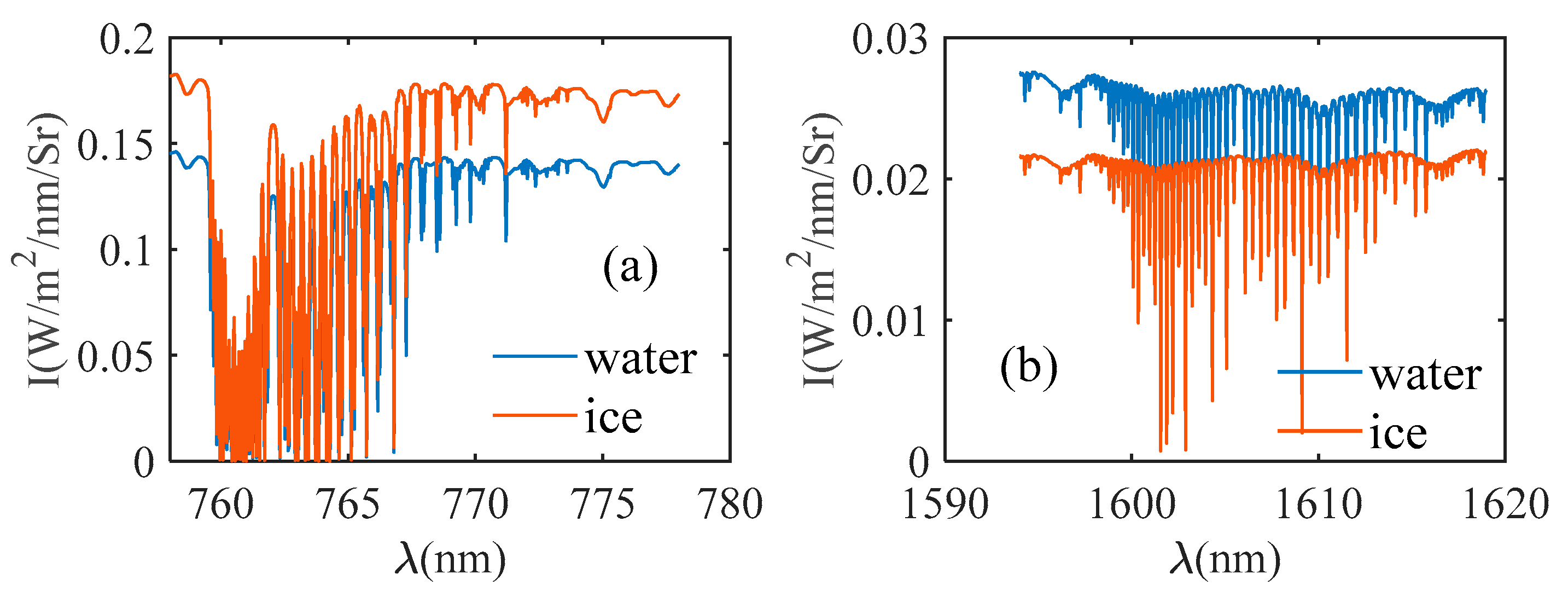
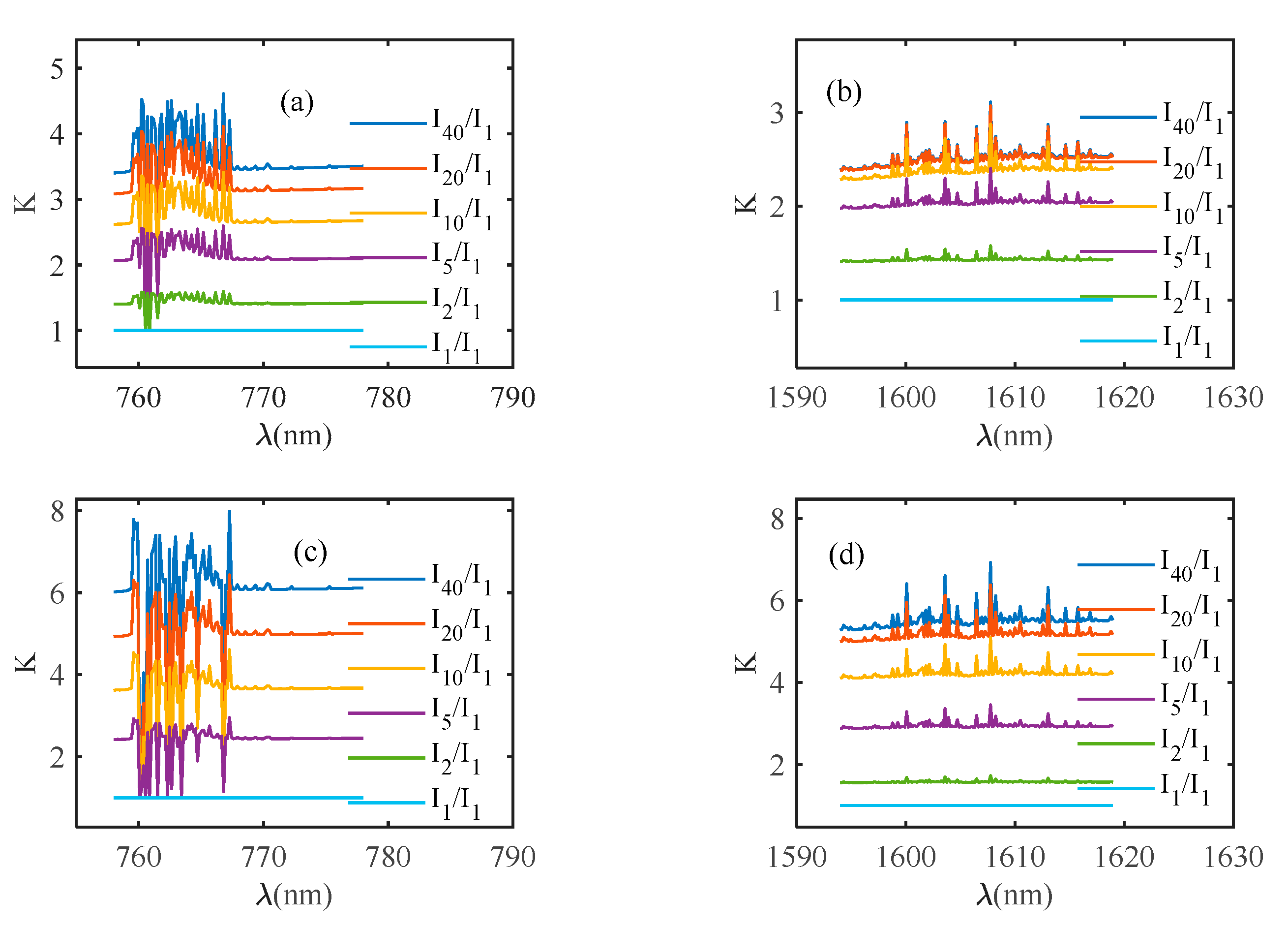
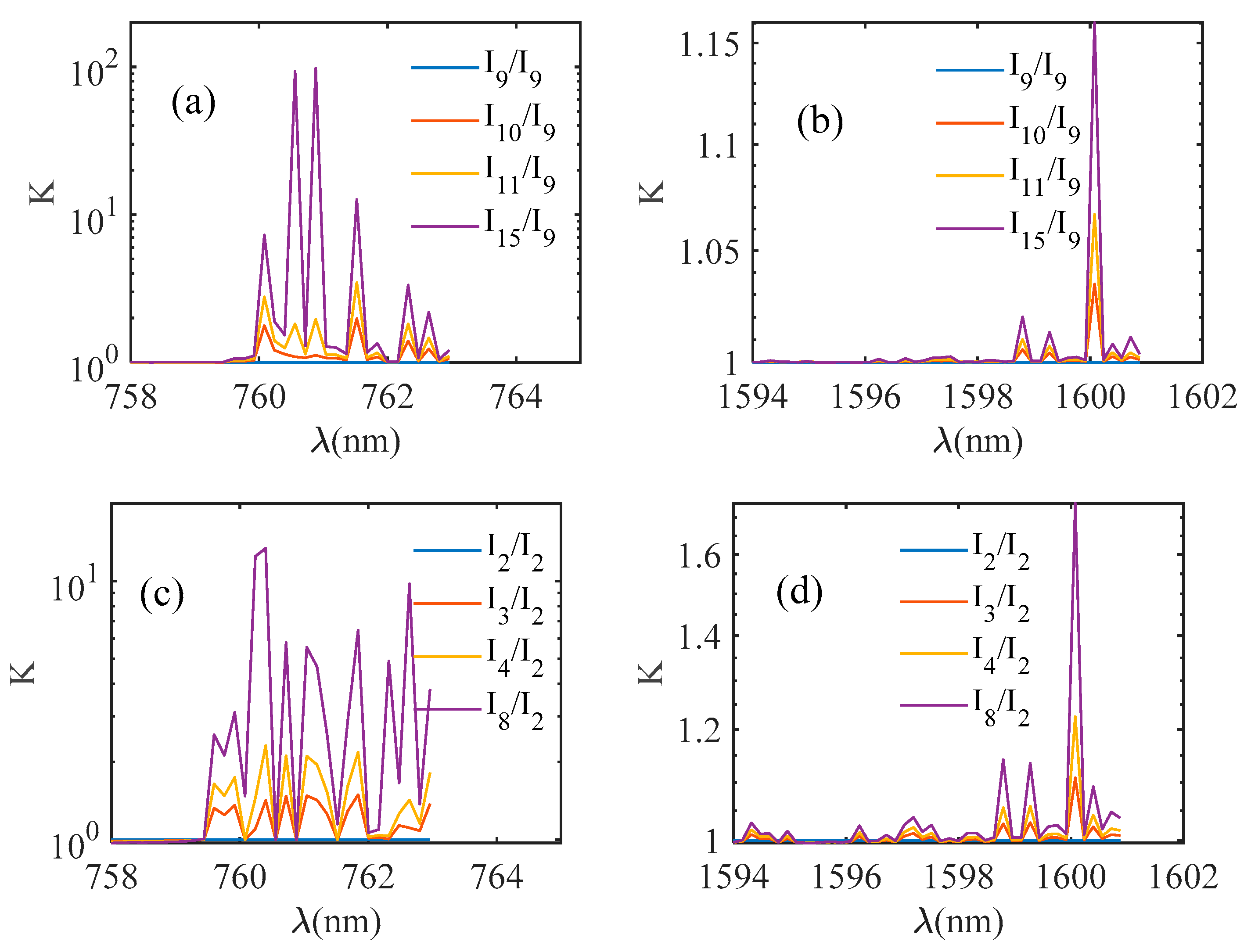
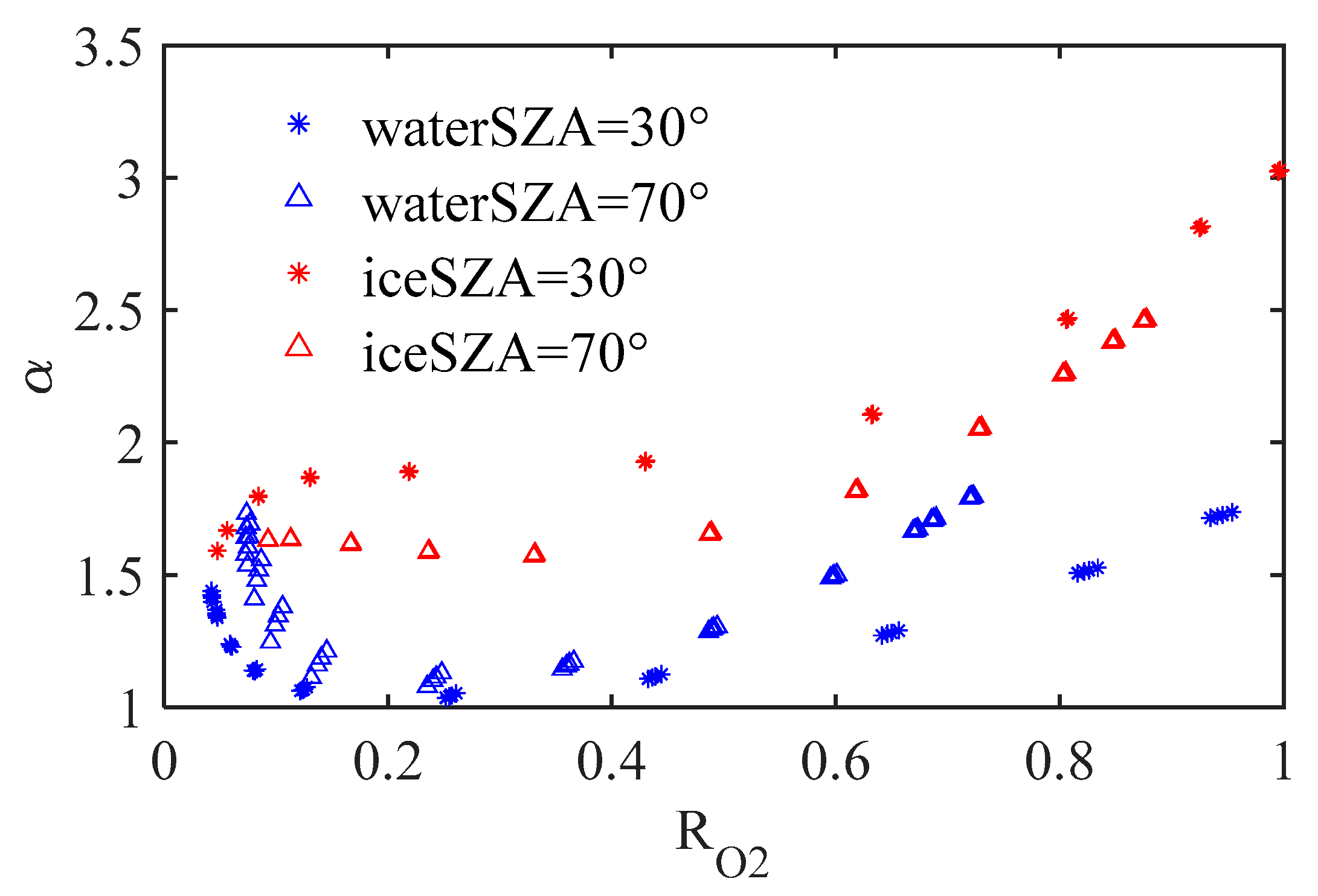
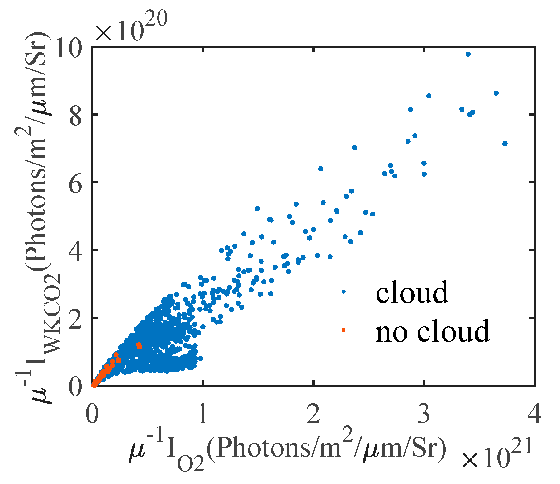
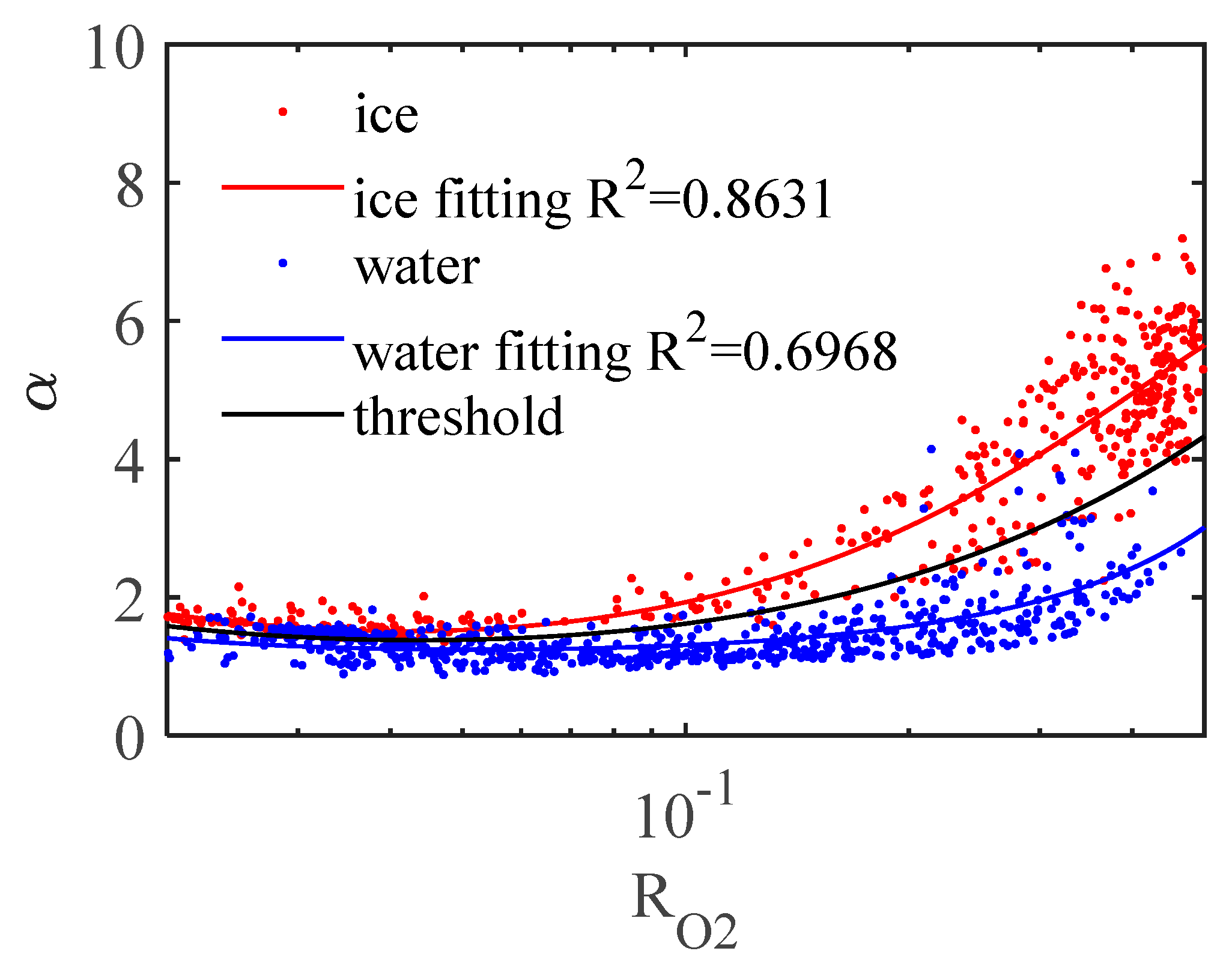
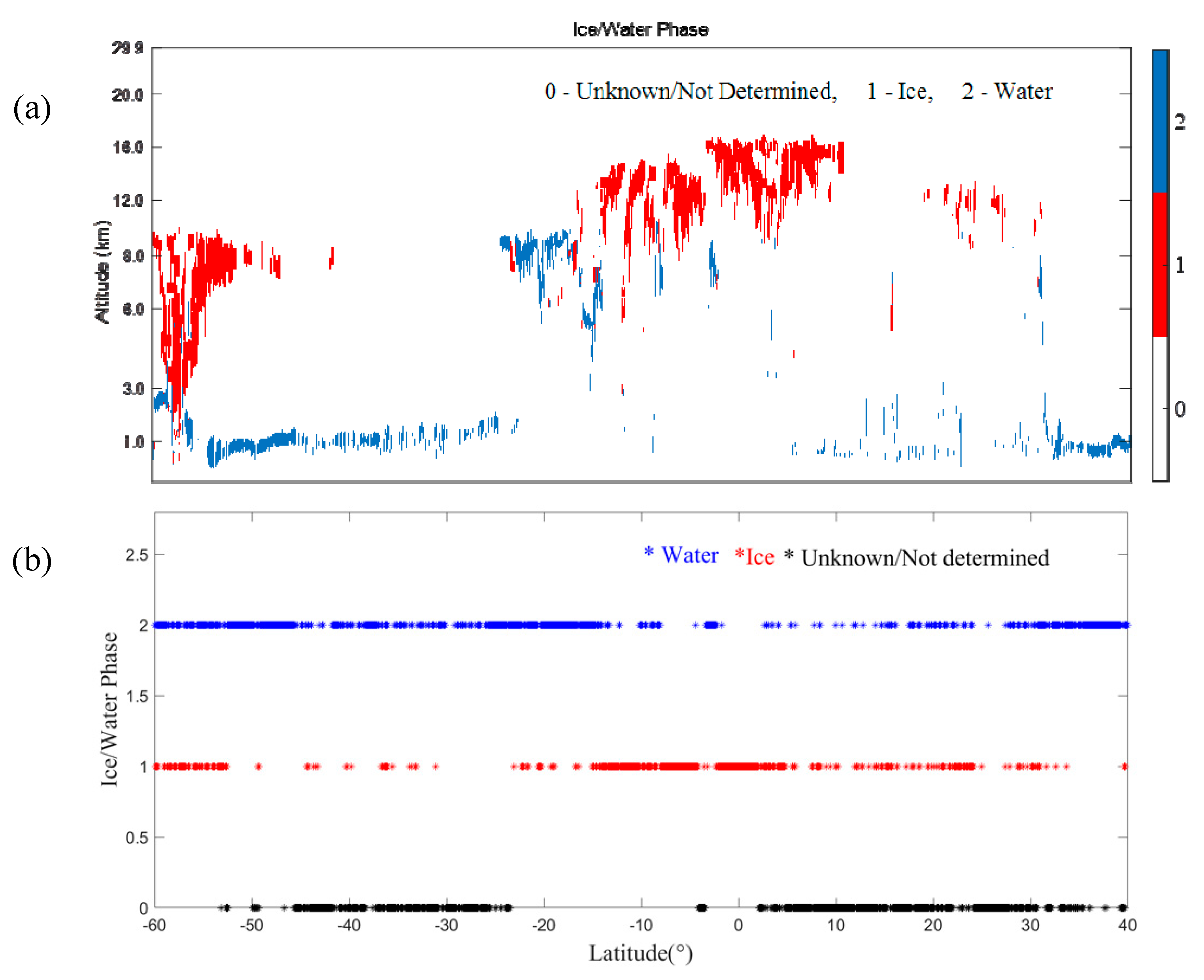
3. Results
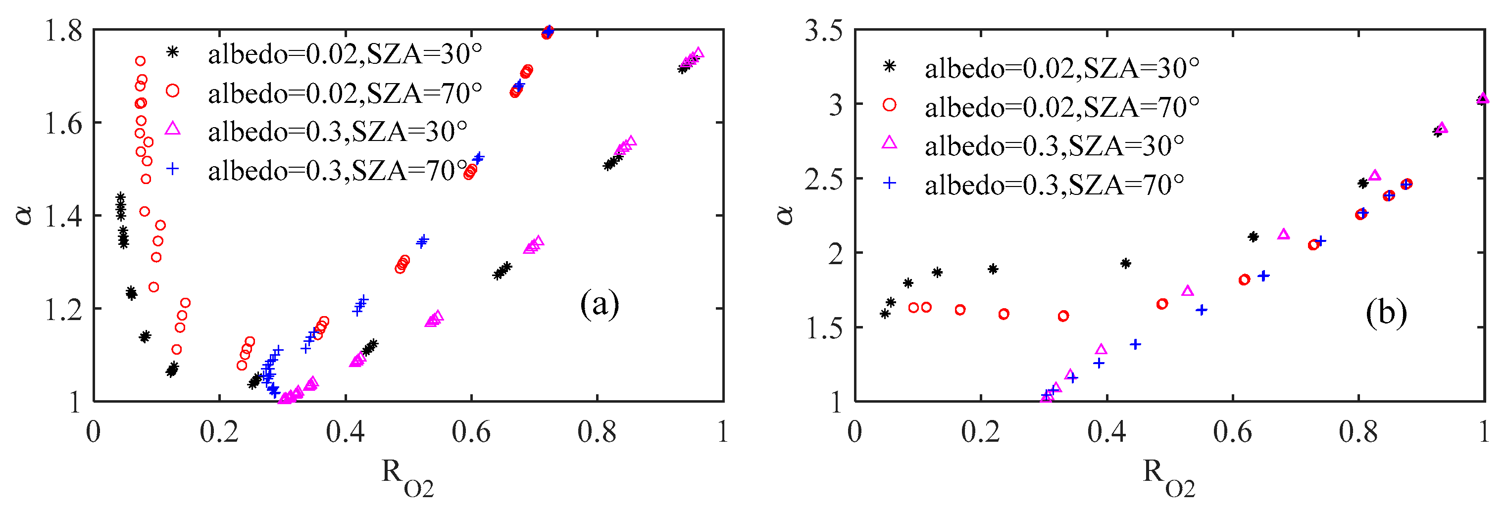
3.1. The Influence of the Solar Zenith Angle on
3.2. The Influence of Surface Albedo on
4. Discussion
5. Conclusions
Author Contributions
Funding
Data Availability Statement
Conflicts of Interest
References
- Kuze, A.; Chance, K.V. Analysis of cloud top height and cloud coverage from satellites using the O2 A and B bands. J. Geophys. Res. Atmos. 1994, 99, 14481–14491. [Google Scholar] [CrossRef] [Green Version]
- Liou, K.N. Influence of Cirrus Clouds on Weather and Climate Processes: A Global Perspective. Mon. Weather Rev. 1986, 114, 1167. [Google Scholar] [CrossRef]
- Li, J.; Yi, Y.; Minnis, P.; Huang, J.; Yan, H.; Ma, Y.; Wang, W.; Ayers, J.K. Radiative effect differences between multi-layered and single-layer clouds derived from CERES, CALIPSO, and CloudSat data. J. Quant. Spectrosc. Radiat. Transf. 2011, 112, 361–375. [Google Scholar] [CrossRef]
- Wetherald, R.T. Cloud Feedback Processes in a General Circulation Model. J. Atmos. 1988, 45, 1397–1416. [Google Scholar] [CrossRef]
- Baker, M.B.; Peter, T. Small-scale cloud processes and climate. Nature 2008, 451, 299–300. [Google Scholar] [CrossRef]
- Trenberth, K.E.; Fasullo, J.T.; Kiehl, J. Earth’s Global Energy Budget. Bull. Am. Meteorol. Soc. 2009, 90, 311–323. [Google Scholar] [CrossRef]
- Dessler, A.E. A Determination of the Cloud Feedback from Climate Variations over the Past Decade. Science 2010, 330, 1523–1527. [Google Scholar] [CrossRef] [PubMed]
- Wang, H.; Su, W. Evaluating and understanding top of the atmosphere cloud radiative effects in Intergovernmental Panel on Climate Change (IPCC) Fifth Assessment Report (AR5) Coupled Model Intercomparison Project Phase 5 (CMIP5) models using satellite observations. J. Geophys. Res. Atmos. 2013, 118, 683–699. [Google Scholar] [CrossRef] [Green Version]
- Stocker, T.; Plattner, G.K.; Dahe, Q. IPCC Climate Change 2013: The Physical Science Basis-Findings and Lessons Learned. In Egu General Assembly Conference; IPCC: Genève, Switzerland, 2014. [Google Scholar]
- Ackerman, T.; Valero, F.; Liou, K. Heating rates in tropical anvils. J. Atmos. Sci. 1986, 45, 1606–1623. [Google Scholar] [CrossRef]
- Hartmann, D.; Ockert-Bell, M.; Michelsen, M. The Effect of Cloud Type on Earth’s Energy Balance: Global Analysis. J. Clim. 1992, 5, 1281–1304. [Google Scholar] [CrossRef] [Green Version]
- Mcfarquhar, G.M.; Cober, S.G. Single-Scattering Properties of Mixed-Phase Arctic Clouds at Solar Wavelengths: Impacts on Radiative Transfer. J. Clim. 2004, 17, 3799–3813. [Google Scholar] [CrossRef]
- Jin, H.; Nasiri, S.L. Evaluation of AIRS cloud-thermodynamic-phase determination with CALIPSO. J. Appl. Meteorol. Climatol. 2014, 53, 1012–1027. [Google Scholar] [CrossRef]
- Baum, B.A.; Menzel, W.P.; Frey, R.A.; Tobin, D.C.; Ping, Y. MODIS Cloud-Top Property Refinements for Collection 6. J. Appl. Meteorol. Clim. 2012, 51, 1145–1163. [Google Scholar] [CrossRef]
- Ackerman, S.A.; Smith, W.L.; Revercomb, H.E.; Spinhirne, J.D. The 27 28 October 1986 FIRE IFO Cirrus Case Study: Spectral Properties of Cirrus Clouds in the 8 12 mum Window. Mon. Weather Rev. 1990, 118, 2377–2388. [Google Scholar] [CrossRef] [Green Version]
- Strabala, K.I.; Ackerman, S.A.; Menzel, W.P. Cloud properties inferred from 8-12m data. J. Appl. Meteorol. 1994, 33, 212–229. [Google Scholar] [CrossRef] [Green Version]
- Jin, H. Satellite Remote Sensing of Mid-Level Clouds. Satellite Remote Sensing of Mid-Level Clouds. Ph.D. Thesis, Texas A&M University, College Station, TX, USA, 2012. [Google Scholar]
- Platnick, S.; King, M.D.; Ackerman, S.A.; Menzel, W.P.; Baum, B.A.; Riédi, J.C.; Frey, R.A. The MODIS cloud products: Algorithms and examples from Terra. IEEE Trans. Geosci. Remote Sens. 2003, 41, 459–473. [Google Scholar] [CrossRef] [Green Version]
- Nasiri, S.L.; Kahn, B.H. Limitations of Bispectral Infrared Cloud Phase Determination and Potential for Improvement. J. Appl. Meteorol. Clim. 2007, 47, 2895–2910. [Google Scholar] [CrossRef]
- Key, J.R.; Intrieri, J.M. Cloud Particle Phase Determination with the AVHRR. J. Appl. Meteorol. 2000, 39, 1797–1804. [Google Scholar] [CrossRef]
- Daniel, J.S. Cloud liquid water and ice measurements from spectrally resolved near-infrared observations: A new technique. J. Geophys. Res. Atmos. 2002, 107, AAC 21-1–AAC 21-16. [Google Scholar] [CrossRef]
- Pilewskie, P.; Twomey, S. Cloud Phase Discrimination by Reflectance Measurements near 1.6 and 2.2 μm. J. Atmos. Sci. 1987, 44, 3419–3420. [Google Scholar] [CrossRef] [Green Version]
- Arking, A.; Childs, J.D. Retrieval of Cloud Cover Parameters from Multispectral Satellite Images. J. Appl. Meteorol. 2003, 24, 322–333. [Google Scholar] [CrossRef] [Green Version]
- Knap, W.H.; Stammes, P.; Koelemeijer, R.B.A. Cloud Thermodynamic-Phase Determination From Near-Infrared Spectra of Reflected Sunlight. J. Atmos. Sci. 2002, 59, 83–96. [Google Scholar] [CrossRef]
- Miller, S.D. Liquid-top mixed-phase cloud detection from shortwave-infrared satellite radiometer observations: A physical basis. J. Geophys. Res. Atmos. 2014, 119, 8245–8267. [Google Scholar] [CrossRef]
- Wang, J.; Liu, C.; Min, M.; Hu, X.; Lu, Q.; Husi, L. Effects and Applications of Satellite Radiometer 2.25- μm Channel on Cloud Property Retrievals. IEEE Trans. Geosci. Remote Sens. 2018, 56, 5207–5216. [Google Scholar] [CrossRef]
- CALIPSO/CALIOP cloud phase discrimination algorithms. J. Atmos. Ocean. Technol. 2009, 26, 2293–2309. [CrossRef] [Green Version]
- Winker, D.M.; Vaughan, M.A.; Omar, A.; Hu, Y.; Powell, K.A.; Liu, Z.; Hunt, W.H.; Young, S.A. Overview of the CALIPSO Mission and CALIOP Data Processing Algorithms. J. Atmos. Ocean. Technol. 2009, 26, 2310–2323. [Google Scholar] [CrossRef]
- Cho, H.M.; Nasiri, S.L.; Yang, P.; Laszlo, I.; Zhao, X.T. Application of CALIOP measurements to the evaluation of cloud phase derived from MODIS infrared channels. J. Appl. Meteorol. Clim. 2009, 48, 2169–2180. [Google Scholar] [CrossRef]
- Richardson, M.; Leinonen, J.; Cronk, H.Q.; Mcduffie, J.; Stephens, G.L. Marine liquid cloud geometric thickness retrieved from OCO-2′s oxygen A-band spectrometer. Atmos. Meas. Tech. 2019, 12, 1717–1737. [Google Scholar] [CrossRef] [Green Version]
- Rozanov, A.; Rozanov, V.; Buchwitz, M.; Kokhanovsky, A.; Burrows, J.P. SCIATRAN 2.0–A new radiative transfer model for geophysical applications in the 175–2400nm spectral region. Adv. Space Res. 2005, 36, 1015–1019. [Google Scholar] [CrossRef]
- Pohl, C.; Rozanov, V.V.; Mei, L.; Burrows, J.P.; Spreen, G. Implementation of an ice crystal single-scattering property database in the radiative transfer model SCIATRAN. J. Quant. Spectrosc. Radiat. Transf. 2020, 253, 107118. [Google Scholar] [CrossRef]
- Eichmann, K.U.; Weber, M.; Heue, K.P.; Leventiduo, E.; Richter, A.; Burrows, J.P. Tropical Upper Tropospheric Ozone Volume Mixing Ratios Retrieved with the Cloud Slicing Method using SCIATRAN/GOME2 data: Methodology, Ozone Sonde Comparisons, and Verification of the new S-5P Operational Processor. In Esa Living Planet Symposium; European Space Agency: Prague, Czech Republic, 2016. [Google Scholar]
- Li, Y.; Zhang, C.; Wang, D.; Chen, J.; Liu, D.; Rong, P. Comparison between the ESFT method and LBL method of CO2 retrieval for high-resolution satellite. In Proceedings of SPIE-The International Society for Optical Engineering; International Society for Optics and Photonics: Bellingham, DC, USA, 2015; Volume 9449. [Google Scholar]
- Liu, D.; Zhang, C.; Li, Y.; Rong, P. The influence of temperature on the simulated high resolution spectra of enhanced SCIATRAN model in near infrared band. Opt. Int. J. Light Electron Opt. 2016, 127, 7292–7299. [Google Scholar] [CrossRef]


Publisher’s Note: MDPI stays neutral with regard to jurisdictional claims in published maps and institutional affiliations. |
© 2021 by the authors. Licensee MDPI, Basel, Switzerland. This article is an open access article distributed under the terms and conditions of the Creative Commons Attribution (CC BY) license (https://creativecommons.org/licenses/by/4.0/).
Share and Cite
Li, Q.; Sun, X.; Wang, X. Cloud Phase Recognition Based on Oxygen A Band and CO2 1.6 µm Band. Remote Sens. 2021, 13, 1681. https://doi.org/10.3390/rs13091681
Li Q, Sun X, Wang X. Cloud Phase Recognition Based on Oxygen A Band and CO2 1.6 µm Band. Remote Sensing. 2021; 13(9):1681. https://doi.org/10.3390/rs13091681
Chicago/Turabian StyleLi, Qinghui, Xuejin Sun, and Xiaolei Wang. 2021. "Cloud Phase Recognition Based on Oxygen A Band and CO2 1.6 µm Band" Remote Sensing 13, no. 9: 1681. https://doi.org/10.3390/rs13091681