Abstract
A large-scale global canopy height map (GCHM) is essential for global forest aboveground biomass estimation. Four GCHMs have recently been built using data from the Geoscience Laser Altimeter System (GLAS) sensor aboard the Ice, Cloud, and land Elevation Satellite (ICESat), along with auxiliary spatial and climate information. The main objectives of this research were to find out how well a selected GCHM agrees with airborne lidar data from locations in the southern United States and to recalibrate that GCHM to more closely match the forest canopy heights found in the region. The airborne lidar resource was built from data collected between 2010 and 2012, available from in-house and publicly available sources, for sites that included a variety of vegetation types across the southern United States. EPA ecoregions were used to provide ecosystem information for the southern United States. The airborne lidar data were pre-processed to provide lidar-derived metrics, and assigned to four height categories—namely, returns from above 0 m, 1 m, 3 m, and 5 m. The assessment phase results indicated that the 90th and 95th percentiles of the airborne lidar height values were well-suited for use in the recalibration phase of the study. Simple linear regression was used to generate a new, recalibrated GCHM. It was concluded that the characterization of the agreement of a selected GCHM with local data, followed by the recalibration of the existing GCHM to the local region, is both viable and essential for future GCHMs in studies conducted at large scales.
1. Introduction
Forest and tree attribute information are required for a wide range of uses, including forest inventory and growth assessment, health monitoring, carbon pool assessments, and informing policy decisions. All of these typically involve volume or biomass estimation. Such data are normally collected in the field and used with or without ancillary conventionally acquired or remotely sensed data—most notably, data obtained from aerial photographs and multi or hyper-spectral imagery. Light detection and ranging (lidar) technologies have been developed over the last thirty or so years, with applications to forests dating at least to the early 21st century [1].
Forest canopy height can be defined as the general level of the canopy of a forested area. To foresters, this would be interpreted as the average height of the dominant and codominant trees in a stand. Previous studies have employed lidar techniques to characterize forest canopy heights, as well as to retrieve forest and individual tree biophysical information, including forest aboveground biomass [2,3,4]. Canopy height models (CHMs) are often generated to predict forest canopy heights. To date, most CHMs have been developed using airborne lidar point cloud data and cover only local-scale areas. For state, national, and international research and decision-making, models covering much larger scales and diverse conditions are required. No comprehensive, large-scale (i.e., national or continental scale) CHM coverage based on airborne lidar data is currently available, and one is not likely to be generated soon, due to cost and feasibility constraints. However, with the high demand of geographically extensive forest studies to retrieve forest biophysical information and estimate forest aboveground biomass, spaceborne lidar data can address such scale issues and can be applied to create comprehensive and economical large-scale CHMs at the regional, national, and continental scales [5,6,7,8].
Canopy height models obtained for very large extents are referred to as “global” canopy height models (GCHMs). Four satellite-based GCHMs have been published, using information derived from the Geoscience Laser Altimeter System (GLAS), the sole instrument on ICESat (Ice, Cloud, and land Elevation Satellite). The GLAS sensor was operational from 2003 to 2009. It (a) produced a very large volume of data, which are still relatively current and worthy of analysis; and (b) offers a unique avenue for investigations aiming to understand the data and developing analysis techniques for other data derived from similar sensors in the future. ICESat has recently been replaced by ICESat-2, which uses a photon-counting sensor [9,10] instead of a GLAS-like waveform-based sensor. GEDI (Global Ecosystem Dynamics Investigation), which was developed by NASA and the University of Maryland, is another new sensor that has been operational since March 2019.
Given the large time gap—up to two decades—between GLAS and these recent spaceborne lidar sensors, calibrating GLAS vegetation height has become relevant for global-scale change detection analysis of canopy heights. Applications that use data acquired from these new sensors will benefit greatly from studies having used ICESat data or from methodologies used to improve GLAS canopy heights. GLAS acquired forest canopy height data using 60 m diameter footprints. The four existing GLAS-based models differ in their approach, application (purpose), vegetation type, and the choice of ancillary data sources. They are, in order of publication: lefGCHM (Lefsky [11]), simGCHM (Simard et al. [12]), losGCHM (Los et al. [13]), and wangGCHM (Wang et al. [14]). Descriptions of these are deferred to the Materials and Methods section. The acronyms are ours. Simard et al. [12] noted large differences between simGCHM and lefGCHM, and attributed many of these differences to their inclusion of land-cover classes with low forest cover densities, such as mosaic crops, open forest, and saline flooded forests. They also noted that simGCHM included a wider range of forest types, which lefGCHM only partially captured; simGCHM displays not only the tall trees in forests, but also shorter woody plants near ground level. The study by Wang et al. [14] generated two mean forest height maps—during spring and summer—and found good agreement with simGCHM (R2 = 0.73 and RMSE = 4.49 m). However, wangGCHM is not considered in our study.
Bolton et al. [15] used 34 small-footprint airborne lidar transects of areas across Canada’s boreal forests for a systematic comparison of lefGCHM and simGCHM. The transects were acquired in 2010 and totaled nearly 25,000 km in length, with a minimum width of 400 m. The data were divided into 25 m × 25 m forested “plots” containing both lefGCHM and simGCHM. The height predictions above 2 m were compared for various ecoregions. They found that simGCHM was in much better agreement with the airborne lidar results than lefGCHM, although the authors were clear in noting that the differences between the definitions, measures, and scales used by the different products may have accounted for at least some of the differences.
Objectives
This work is part of a larger project, for which the overarching objective was the creation of a regional forest biomass map. As studies begin to utilize ICESat-2 (and, especially, GEDI satellite data), this research is meant to provide a simple methodology for evaluating the accuracy of GCHM products in areas where data of equal or better quality are available (e.g., airborne lidar point cloud data). Similar calibration functions could be employed to make such GCHM products more useful for estimating biomass and other biophysical parameters in areas with similar ecological characteristics (e.g., as in ecoregions), and for assessing the veracity of the resulting predicted products (e.g., maps). As Bolton et al. [15] have demonstrated, for products derived from a very large-scale area, the initial calibration might benefit from recalibration using data specific to an area of interest.
Being large-scale in nature, one of the main questions for the larger project centered on the creation of a regional forest height product on which the biomass product would depend. This led to the main objective of the study documented herein; namely, to assess the efficacy of localizing (i.e., regionalizing) an existing global forest canopy height model to the forests of the southern United States. The particular objectives of this study were to: (1) select one of the GCHMs, based on a qualitative evaluation of their strengths and weaknesses; (2a) develop a method by which to evaluate the selected GCHM more thoroughly and quantitatively and, in doing so, to ascertain the veracity of the selected GCHM; (2b) select airborne lidar point cloud metrics that are closely associated with the selected GCHM and that can be used in the production of prototype regionalized maps; and, finally, (3) quantitatively and qualitatively compare the new models (maps) with the GCHM selected in (1). Objectives (2a) and (2b) are inextricably intertwined and can be viewed as a pair of dual sub-objectives.
2. Materials and Methods
In this section, we provide details of the steps taken in conducting this research. The overall approach is summarized in Figure 1.
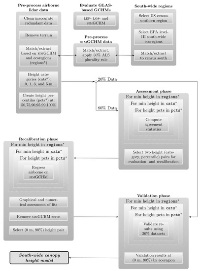
Figure 1.
Workflow diagram indicating the interplay between airborne lidar data and simGCHM as data sources, as well as the analysis phases used in the creation of swCHM.
2.1. Study Area
This study concerns the forests of the southern United States, a region defined by the United States Census Bureau [16] as the sixteen states identified in Figure 2. It coincides with the USDA Forest Service’s thirteen-state Southern Region, with the exclusion of Puerto Rico and the inclusion of West Virginia, Maryland, Delaware, and the District of Columbia. We selected the Census Bureau definition over that of the Forest Service due to the presence of several airborne lidar collection sites in Maryland. The Southern Region is a large area with a wide variety of vegetation, influenced by the climate, geology, hydrology, past and current land uses, native and introduced plant species, and so on, all of which can be considered at several levels of specificity [17].
As regression analyses were used to associate local airborne lidar-based canopy height information with canopy heights obtained from existing GCHMs, it was necessary to reduce within-regression domain variances. This was achieved through stratifying by ecoregion. In particular, the sixteen-state Southern Region of the US Bureau of Census was further classified into ecoregions, according to the United States Environmental Protection Agency (EPA)’s level III ecosystem classification system [18].
The EPA has created a hierarchical system for ecosystem classification, which attempts to group ecosystems into ecoregions based on the type, quality, and quantity of environmental resources therein [18,19]. There are four levels to the hierarchy, creating a range in coarseness and, hence, in the number of sub-regions included at each level. To determine the appropriate ecoregion level (I–IV) for use in addressing project objectives, the scales and the number of ecoregions associated with each south-wide EPA ecoregion-level was considered. Levels I and II, with three and four south-wide ecoregions, respectively, were eliminated, as those ecoregion definitions were too broadly defined for our purposes. Conversely, the level IV categorization was much too fine, with 220 south-wide ecoregions. Thus, we chose to work with the level III categorization. The gray lines in Figure 2 depict the 34 south-wide EPA level III ecoregion boundaries.
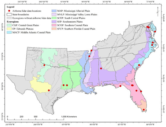
Figure 2.
EPA level III ecoregions [20] and airborne lidar point cloud data locations (red dots) superimposed on the states comprising the United States Census Bureau Southern Region. Colored areas represent the effective study area used in this research.
Our particular objectives concerned the use of existing airborne lidar data for the south-wide regionalization of a GCHM, and, thus, the effective area of interest was further reduced by the availability and locations of existing airborne lidar collection sites. These are shown, in Figure 2, as red circles and are described below. The nine colored (non-gray) regions of the figure correspond to nine EPA level III ecoregions containing one or more airborne lidar collection site(s). Hence, the nine colored EPA level III ecoregions effectively defined our study area. Large portions of Texas, Oklahoma, Arkansas, Tennessee, Kentucky, North Carolina, Virginia, and Maryland were excluded, due to a paucity of airborne lidar sites in the ecoregions therein; West Virginia was completely excluded. Only Mississippi, Florida, and Delaware were completely contained within one or more ecoregions; however, none of the project airborne lidar collection sites were located in either Mississippi or Delaware. Table 1 provides the EPA abbreviations, names, and the number of regressive cells with (n) and without (n′) simGCHM zeros for each of the nine ecoregions present in our data; Table 2 presents a brief description, paraphrased from Wiken [18], of each ecoregion.

Table 1.
Ecoregion codes and names, the total number, and the number of regressable cells with (n) and without (n′) simGCHM zeros.
Table 2.
Brief ecoregion descriptions; adapted from Wiken et al. [18].
2.2. Selection of the Reference GCHM
As mentioned in the Introduction, four potential GCHMs that used GLAS-derived data from the time that that sensor was operational were available, but wangGCHM was excluded. Brief descriptions of the other three, with a focus on simGCHM, are as follows:
- lefGCHM (acronym ours). Lefsky [11] combined data from both the GLAS and the Moderate Resolution Imaging Spectroradiometer (MODIS) sensor systems. Ground data from four forested sites in the United States and three in the Brazilian Amazon were used for GLAS data calibration. MODIS data were used for stratification and attribution of forest patches. This attribution, together with the globally available GLAS and MODIS data, then allowed for global prediction of forest canopy heights. The focus of Lefsky [11] was on methodological development; it stands out as the first GCHM to reveal the distribution of forest canopy height globally. It was later employed, by Saatchi et al. [21], to investigate tropical forest carbon stock across three continents.
- simGCHM. Simard et al. [12] integrated GLAS RH100-derived estimates of canopy height from the GLA14 land product for 2005 with various forest, tree, topographical, and climatic variables in order to generate a wall-to-wall global canopy height map. RH100 values are defined as the distance between the beginning of the laser pulse-echo and the corresponding location of the ground peak [22,23,24], thus representing vegetation canopy height. As with lefGCHM, the generation of simGCHM was primarily method-oriented.
Data ancillary to simGCHM include mean annual temperature and precipitation, as well as temperature and precipitation seasonality information from the Tropical Rainfall Measurement Mission (TRMM) [25] and the Worldclim [26] datasets. Also included were coincident Shuttle Radar Topography Mission (SRTM) [27,28] elevation, MODIS tree cover data (MOD44 map) [29], and forest class information from the Globcover map [30], as well as information concerning the protection status of forest sites (United Nations). The latter was included with the assumption that protected sites have a lower error rate, due to lower variability in canopy heights.
Simard et al. [12] argued that the segmentation procedure of MODIS reflectance data used by Lefsky [11] to delineate forest patches produced results that can be difficult to interpret. They based this argument on the facts that “(i) [the] MODIS images were segmented based on spectral/textural heterogeneity thresholds that do not readily translate into the forest stand properties, and (ii) model error can be attributed to both sub-pixel (500 m MODIS) and sub-patch (1–900 MODIS pixels) variability” (p. 1). Instead of the forest patch approach taken by Lefsky [11], Simard et al. [12] chose to associate selected GLAS shots with 1 km × 1 km pixels, as “we believe that in the absence of high-resolution forest disturbance/age maps to serve as segments, the pixel approach deserves evaluation” (ibid).
The lidar waveforms used for simGCHM development were selected from forested sites, as defined by the Globcover map [30], in a manner designed to reduce the impact of slope and cloud contamination on canopy height estimates. Calibration (and validation) of the RH100-derived lidar waveforms was performed using a set of 98 co-located field sites in tropical ecosystems in Uganda, Africa, during September 2008. The heights of the three tallest trees within the plot were measured using a clinometer. The decision to use only the three tallest trees was made in an attempt to minimize the effect of roughness. The Random Forest algorithm [31,32], a non-parametric algorithm often used in the context of machine learning, was used for all model fitting. The Uganda data, together with canopy height data from the FLUXNET La Thuille database [33,34], were used for simGCHM model validation and uncertainty assessment.
- losGCHM. Like Lefsky [11], Los et al. [13] combined GLAS and MODIS data; furthermore, like Simard et al. [9], they also included SRTM-derived data. With these data, they created coarse-resolution (0.5° × 0.5°) vegetation height and vegetation cover fraction products for latitudes between 60° S and 60° N. The authors stated that the maps were created for use in climate and ecological models but did not, themselves, develop a particular application. losGCHM has been used, by Bevan et al. [35], to investigate the response of vegetation after the 2003 European drought.
Los et al. [13] identified four specific objectives in creating their map; only the third—to develop and test a near-global vegetation height model—was directly related to this paper. The other three objectives included the initial testing of the underlying vegetation height model [36]; the development of filters to reduce the effects of clouds, aerosols, and topography on GLAS-derived vegetation height estimates; and the development of bare soil and tree cover fractions from the GLAS-produced tree height product.
To evaluate the efficacy of regionalizing an existing publicly available global canopy height model to the forests of the southern United States, lefGCHM, simGCHM, and losGCHM were compared, based on their scientific reports. lefGCHM was the first of the three models described above to be produced, followed by simGCHM and, finally, by losGCHM. All three models are publicly available, at least as the final map product.
As mentioned in the Introduction, Simard et al. [12] noted large differences between simGCHM and lefGCHM, as well as the fact that simGCHM includes a wider range of forest types that lefGCHM only partially captures. simGCHM displays not only the tall trees in forests, but also shorter woody plants near ground-level. Due to its very large (0.5° × 0.5°) cell size, the second constraint essentially removed losGCHM from contention, leaving only lefGCHM and simGCHM.
lefGCHM shows a large presence of non-legend white for the Southern Region of the United States, indicating that these locations were not modeled by Lefsky, presumably due to missing data. simGCHM (Figure 3) has far fewer missing values, strongly favoring simGCHM over lefGCHM, in terms of coverage of the south-wide forests. Perhaps even more convincing is the strong visual alignment between the simGCHM canopy heights and the EPA level III ecoregions, as seen in Figure 3. For example, in Figure 2, we can see that the South Central Plains (SCEP) covers parts of Texas, Louisiana, Arkansas, and Oklahoma. In Figure 3, this area is dominated by orange and bright yellow “paint”, indicating relatively tall canopies. The adjacent Mississippi Alluvial Plain (MAP) is pinker and blotchier, indicating shorter and generally more variable canopies. To its east, canopies of the Mississippi Valley Loess Plain are again taller. Similarly, the Southern Florida Coastal Plain (SFCP) is smoother and shorter than that of the Southern Coastal Plain (SCOP) to its north. To our knowledge, Simard et al. did not consult the EPA regional map when creating simGCHM.
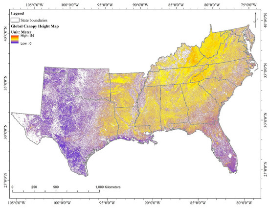
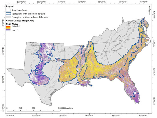
Figure 3.
Top panel, simGCHM (Simard et al. [12]) restricted to the southern United States. EPA level III ecoregions [20]; bottom panel, simGCHM restricted to the nine EPA ecoregions used in this study.
The recalibration approach adopted herein was used to rescale existing map values to a particular region, through the use of local, better resolution (and, presumably, better quality) data. As such, the cell size of the selected map product, not the initial data from which that map was derived, determined the nominal resolution of the recalibrated map. Simard et al. [12] used 1 km2 pixels; Lefsky [11] used forest patches which ranged from about 0.25 km2 to 225 km2, with a mean of about 25 km2 globally. Simard et al. [12] (p.1) provided a convincing argument in favor of their 1 km2 pixels over the lefGCHM patches. Consistently sized pixels, such as those of simGCHM, may also be more consistent with regression analyses, if long runs of gridded, like-valued, and patch-based attributes were to be observed. Finally, while both Simard et al. [12] and Bolton et al. [15] provided the caveat that differences in methodologies need to be considered when comparing lefGCHM and simGCHM, both papers found simGCHM to be superior to lefGCHM.
In short, we chose simGCHM (Figure 3) as our reference GCHM, due to its proper spatial resolution, the large forest areas that it covers, visual agreement with the EPA level III regions, and its public availability on the NASA Jet Propulsion Laboratory website (Global 1 km Forest Canopy Height) [37].
2.3. The Airborne Lidar Data
Existing airborne lidar data from publicly available sources were used for this research. Sources included: (1) NASA’s Goddard’s LiDAR, Hyperspectral, and Thermal Image (G-LiHT) program [38]; (2) the National Ecological Observatory Network’s (NEON) prototype data sharing program [39]; (3) the NSF OpenTopography program [40]; and (4) the Lidar Applications for the Study of Ecosystem with Remote Sensing (LASERS) Laboratory, Department of Ecosystem Science and Management, Texas A&M University. The scanning locations of these airborne lidar collections were distributed (albeit not randomly nor evenly) throughout the study area. They included sites in Alabama, Arkansas–Tennessee, Florida, Maryland, Mississippi, North Carolina, South Carolina, and Texas (Table 3); thus, by construction, including all nine of the study area ecoregions.
Table 3.
Airborne lidar collection sources, states, ecoregions, and dates.
All data were from 2010–2012, except that for Merritt Island, FL (2008). These dates were selected for consistency with the dates of operation of the GLAS sensor, upon which simGCHM depended, and with the 2010 publication of simGCHM. To avoid the necessity of pixel weighting for unbiased estimation, the aerial extent of the airborne lidar data was further restricted to cells completely covered by simGCHM. This was in contrast with the study of Bolton et al. [15], in which partially covered pixels were used. As such, the airborne lidar data required cleaning and pre-processing before calculating airborne lidar metrics and assessing the accuracy of simGCHM.
The first step in cleaning and pre-processing the data was to remove terrain heights to produce canopy heights. A 3 m DEM (9 m2) was created in-house, using the airborne lidar data. Then, the DEM terrain values were subtracted from airborne lidar point heights to produce canopy heights [41]. Raw airborne lidar data can be subject to knowable errors, such as having very unlikely positive elevations (e.g., returns from communication towers) or having apparent negative elevations after terrain height removal. Moreover, Simard et al. [12] stratified their data to correspond with forested areas, and our objective was the creation of a CHM for the Southern Region of the United States. Therefore, we displayed our point cloud data along with Google Earth historical images and aerial photos and used operator experience to identify and remove negative post-DEM returns and returns for areas or objects likely in error or outside of our population of interest, including agricultural land, lakes, and so on.
2.3.1. Height Categories
Once the airborne lidar data was cleaned, four separate data sets were generated in an attempt to evaluate the influence of lesser vegetation, such as grasses and brushes, on upper canopy relationships. Each of the four datasets contained airborne lidar data having values greater than a specified minimum height. We refer to these as minimum height categories (or, simply, height categories). They were defined as follows:
- 0 m ≔ All airborne lidar points (include all ground points);
- 1 m ≔ Points greater than 1 m (without ground, short grass, and rock points);
- 3 m ≔ Points greater than 3 m (without ground, short/tall grass, rock, and short shrub points), and
- 5 m ≔ Points greater than 5 m (without ground, short/tall grass, rock, and short/tall shrub points).
The leading numeral and unit identify each minimum height category. Bolton et al. [15] used a 2 m minimum height category.
2.3.2. Plurality Rule and Height Percentiles
The Quick Terrain Modeler Generate Outline algorithm—Applied Imagery—was used to create perimeters around the (x, y) co-ordinates of the lidar point cloud data, separately for each ecoregion. The ESRI ArcGIS Extract by Mask tool was then used to associate the accumulated airborne lidar with a unique simGCHM pixel. This tool used a fixed value of 50%, whereby any pixel having less than 50% overlap with the airborne lidar data was excluded from the output. In effect, together with the fact that non-forested areas were excluded from simGCHM, this guarantees that each resultant output cell was both forested in the simGCHM sense and had a generalized (outlined) airborne lidar coverage of at least 0.5 km2. It also provides that there was a sufficient number of lidar points associated with most pixels for the accumulation of reliable height percentile statistics. It was considered beyond the scope of this study to experiment with minimum coverage assumptions and the quality of the resultant statistics.
For each pixel passing this 50% plurality rule, we computed the mean and mode height values and the following height percentiles: 50, 60, 75, 90, 95, 99, and 100 (i.e., maximum height). The median and mode were irrelevant to our conclusions and are not considered herein. By the “pth height percentile”, we mean the height, h, for which p percent of the lidar returns associated with a particular simGCHM pixel were from aboveground heights of h m or less. Percentile heights have been frequently adopted in studies utilizing airborne lidar information, as percentiles are more resistant to outliers than, say, means are; including noise associated with high-elevation returns. Percentile heights from lidar provide rich information describing the vertical structure of vegetation, canopy height, and biomass [42]. Bolton et al. [15] used 95th percentile heights.
Individual analyses were performed for pairs of height percentiles and height categories—that is, for all 8 × 4 combinations of height percentiles and minimum height categories.
2.4. Analysis
The analysis consisted of two main components: (1) to sequentially ascertain the efficacy of simGCHM and, assuming its efficacy, to produce a set of response (i.e., dependent) variables for use in the localization of the simGCHM to the Southern Region of the United States; and (2) to realize that localization by regressing the selected airborne lidar values on the associated simGCHM pixel values, thus recalibrating the simGCHM to the south-wide ecoregions. We refer to these two components as the assessment and recalibration phases of the overall study.
The two datasets—simGCHM and the airborne lidar—were each randomly split, such that 80% of each was used for both assessment and recalibration, while 20% was withheld for subsequent evaluation of the results. In the literature, the term “calibration” data is normally used for the former. To avoid confusion with our use of “recalibration”—in the sense of rescaling the Simard et al. [12] product to better fit the southern United States—we sometimes refer to this 80% set as the “estimation” data. Similarly, we variously refer to the latter set as the “validation” data. While both sets played a role in each phase of this study, the primary use of the 20% validation set was for validation of the final model, and only those results are presented herein.
2.4.1. Assessment Phase
The metrics used to address (1), above, were those listed in the previous section; namely, height percentiles at the 50, 60, 70, 75, 90, 95, 99, and 100th (maximum) percentiles, and minimum height categories at 0, 1, 3, and 5 m, all of which were obtained from the airborne lidar point clouds for the corresponding ecoregion. Each was accumulated and assessed against the associated simGCHM pixel-based canopy height value. In addition to the per-ecoregion analyses, the data were also accumulated across all the ecoregions for an overall assessment.
As for the statistics, Bolton et al. [15] noted that “conventionally, bias and RMSE are used to compare model predicted values against measured values to assess the accuracy of a model. Here, these metrics were not used to assess model accuracy, but simply to assess the agreement between two predictions (i.e., GLAS predictions against airborne Lidar derived predictions of canopy height)”. They used the word “agreement” in the title of the paper in question, yet still referred to “bias” and “RMSE” throughout the body of the paper. “Bias” has several meanings; the statistical definition is intimately tied to probability distributions, while the “engineering” meaning generally accepts the measured value to be true, or closer to the truth, than the predicted value. When both values are predictions, the water becomes murkier. We agree with Bolton et al.’s comment referring to bias and agreement and while, in the assessment phase of this study, we used the same formula as Bolton et al. and many others have, we took the issue a bit further and adopted the expression “mean agreement” for what is conventionally called “bias” in the lidar literature. A similar argument pertains to RMSE, for which we adopted a formula that is very closely related to the usual RMSE formula, which we call the “mean absolute agreement”; it has the same units, roughly the same geometric meaning, and is to be interpreted in the same way as what is usually called RMSE.
Let represent airborne lidar values (height category j, height percentile ) for pixel i, in ecoregion simGCHM values. Furthermore, let be the number of pixels in ecoregion having an value. The could potentially differ for some (pixel, ecoregion) pairs, due to the height category definition. This was an unlikely scenario, due to the simGCHM stratification to forests and adherence to the 50% plurality rule; indeed, it did not occur. Further, the are the same for all j and k, so we simplified the notation by letting and for all j and k. Then, is an estimate of how well the two canopy height estimates agree for measure in pixel i for ecoregion . The mean agreement (MA), also known as the “bias”, then, is simply:
and we define the mean absolute agreement (MAA) as:
Equations (1) and (2) are closely related. For comparison, the more conventional RMSE is defined as:
An informal comparison of and values indicated that, for canopy height values, the two expressions are measuring essentially the same quantities.
The 80% estimation dataset was used to assess and , primarily by graphical methods. Prior to making final decisions as to which of the airborne lidar metrics was to advance to the next phase of the analysis, several studies [1,15,43,44,45,46] were consulted in order to check the priority and reasonableness of the selected measures.
2.4.2. Recalibration Phase
Simple linear regression was used for each ecoregion and height percentile x category pair; specifically,
Recall that there are implied subscripts on the simGCHM variable. Standard regression diagnostics, including graphics, were consulted to assess the reasonableness of the regressions and interpretation of the results. Initially, all of the 80% estimation data were used. Following preliminary evaluation, this was modified to non-zero simGCHM values only. There were, by definition, no airborne lidar percentile heights equal to zero. The assessment phase was not repeated after the removal of the simGCHM zeros.
2.4.3. Validation Phase
The validation phase consisted of three inter-related tasks; simGCHM zeros in the 20% validation dataset were removed before conducting these tasks. The tasks were as follows: firstly the classical approach of computing the “bias” and root mean squared errors from the regressions of the recalibration phase were calculated for the 20% validation dataset. For the validation phase, we revert to the more usual term, “bias”, rather than agreement, as we compared the 20% validation data to corresponding data, for which the differences were assumed to be completely random. We calculated both the RMSE and mean absolute “errors”, according to Equations (3) and (2), respectively.
Secondly, regression models were fit to just the 20% validation data. Thirdly, maps were created using those results, for direct comparison with the results of the 80% recalibration dataset. These 20% based ecoregion-specific results were visually compared to their 80% counterparts. As the decision to favor the airborne lidar height pair (0 m, 90th) pair had already been made, the second and third tasks were conducted only for that pair of measures.
3. Results
3.1. Assessment Phase
Figure 4 and Figure 5, respectively, depict the assessment-phase mean agreement (MA) and mean absolute agreement (MAA) values between simGCHM and the airborne lidar data. The four panels in each figure are for the 0 m (upper left), 1 m (upper right), 3 m (lower left), and 5 m (lower right) height categories. Each of the nine ecoregions, as well as all ecoregions combined, are represented in the panels by different colors, as identified in the legend. In each case, the horizontal axes represent height percentiles, with specific MA or MAA values (vertical axes), plotted on the 50, 75, 90, 95, 99, and 100 height percentiles. Values at 60th and 70th percentiles were omitted, in order to reduce clutter. Smoothing splines were used simply to help visualize the relationships; any “blips,” as in the CGP curve (dark blue) near the 99th percentile of the 0 m height category panel (upper left) of Figure 5, are artifacts of discontinuities in the data and should largely be ignored.
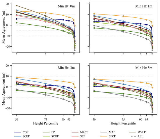
Figure 4.
Mean agreement (MA) statistics by ecoregion (individual spline-fitted lines), height percentiles (horizontal axes), and minimum height categories (panels) computed during the assessment phase of the study. The spline-fits are strictly for visual display.
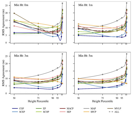
Figure 5.
Mean absolute agreement (MAA) statistics by ecoregion (individual spline-fitted lines), height percentiles (horizontal axes), and minimum height categories (panels) computed during the assessment phase of the study. The spline-fits are strictly for visual display.
The overall shapes of the relationships in the four panels of Figure 4, for MA, in general, were quite similar; as were those for the MAA panels in Figure 5. Within each of the height category panels of Figure 4, we can observe a gradual decrease in mean agreement values, from generally positive values (SIMGCHM canopy height values larger than the corresponding airborne lidar values) at the 50th percentile to generally negative values by the 95th percentile, as well as from the 0 m height category to the 5 m category. These observations make sense: as the minimum height category increases, fewer lesser vegetation points are included in the point cloud summaries and, so, the percentile height per pixel increases, resulting in a decrease in the simGCHM minus the airborne lidar values. Similarly, for a given minimum height, as the percentile of height increases, a larger percentage of the taller trees contribute to the per-pixel statistics, such that the airborne lidar values again increase, decreasing the associated MA values.
For the 5 m minimum height category, the MA trajectories were roughly centered about zero for the 75th percentile height class. In all cases, by the 99th percentile, we can see a very sharp decline and almost consistently negative values (airborne lidar values larger than those of simGCHM). We can also see that, for most ecoregions, the mean agreement values were largest for the 0 m height categories and decreased consistently through the 5 m categories. This is consistent with intuition: if vegetation up to 5 m has been removed from the point cloud data, then the percentile “pixel height” of the remaining trees will often be considerably higher than the percentile height with the lesser vegetation included. The associated simGCHM value for the associated pixels was fixed, so the simGCHM minus the point cloud value must decrease.
The overall shapes of the curves suggested that the 0 m height category paired with the 90th percentile should be near-optimal. Prior to making final decisions as to which airborne lidar metrics were to advance to the next phase of the analysis, a number of previous studies [1,15,43,44,45,46] were consulted in order to check the priority and reasonableness of the selected airborne lidar metrics. As a number of investigators, including Bolton et al. [15], used the 95th percentile, we included it as well.
3.2. Recalibration Phase
Figure 6 displays the scatter of the airborne lidar 0 m, 90th percentile heights, plotted against the corresponding simGCHM canopy heights for each ecoregion (panel)—excluding EP—and for all ecoregions combined. Plots for the 95th percentile data were similar and, therefore, omitted. The plot for EP was uninteresting, due to its paucity of data (total of seven points, five of which were at the simGCHM origin). In each panel, dotted lines indicate the respective means and dashed lines are the 0–1 (intercept and slope) lines. Equation (4), relating the simGCHM height values to those of the corresponding airborne lidar percentile values, was fitted separately by ecoregions and to ecoregions combined. Ecoregion-specific results for the 90th percentile data are shown, in Figure 6, as purple lines, while the statistics associated with Equation (4), for both the 90th and 95th percentile heights, are presented in the upper portion of Table 4.
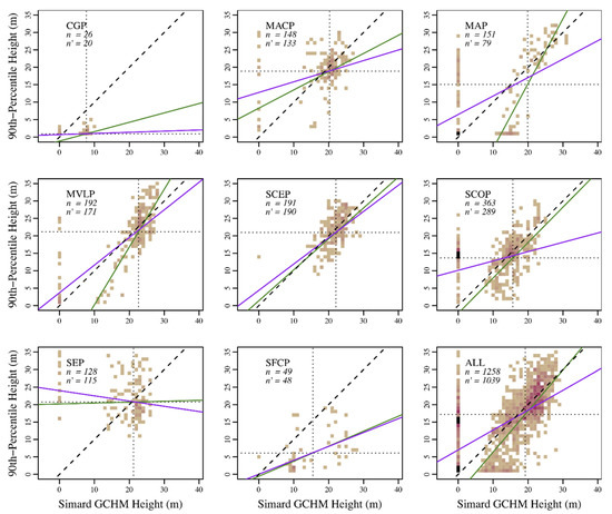
Figure 6.
Scatterplots and fitted models for each ecoregion (except for EP) and for all regions combined; simGCHM-zeros were included/excluded for the purple/green fits (with sizes of n and n′, respectively). The associated statistics are provided in Table 4. Dotted lines indicate the respective means and dashed lines indicate the 0–1 lines. The color represents the number of data points, with tan as 1, maroon up to 16, and black more than 16. The maximum was 44 points at simGCHM = 0 and airborne lidar 90th percentile heights less than 1 m, for all data combined.
Table 4.
Regression coefficient estimates and associated basic statistics for regressions, including (upper panel) and excluding (lower panel) simGCHM zero height values. Values to the left/right are for the 90th and 95th airborne lidar height percentiles; all regressions are for the 0 m airborne lidar height category.
What stands out the most in Figure 6 is the large number of simGCHM zeros in most ecoregions. The fact that most of those zeros were not clustered with small values of the associated percentile data indicates that simGCHM zeros are from different sub-populations and should not be used in these regressions. As there was no way to disentangle what may be true zeros from what may be spurious zeros, the regressions were refitted without the simGCHM zeros. Standard regression results for the 90th and the 95th percentiles for each ecoregion are shown in the lower portion of Table 4.
Entries in the lower portion of Table 4 indicate that the intercepts for four of the nine ecoregions—CGP, SCEP, SCOP, and SFCP—were not significantly different from zero and that the slopes were all significantly different from zero, except for those of CGP and SEP. The Central Great Plains (CGP) is not heavily forested and had few pixels available for regression. simGCHM pixel values for the CGP were all less than about 10 and the airborne lidar heights for this ecoregion were all less than about 5, so it is not surprising that neither coefficient associated with this region was significantly different from zero. As for the SEP (Southeastern Plains), this ecoregion is quite varied, with tall, large, and short vegetation and a variety of land uses. The large trees to the west accounted for the intercepts significantly different from zero, and it is likely that the zero slopes were associated with mixed vegetation and land use within simGCHM’s 1 km2 pixels.
While knowledge of the p-values reported in standard regression outputs is useful, the associated tests do not address the questions most pertinent to this research. Recall that these tests are associated with the null hypothesis that the coefficients under consideration are, individually, not different from zero. In our case, the chance that both the slope and the intercept were both zeros is extremely small for forested ecosystems—as such, we expected that the percentile heights tracked the simGCHM heights fairly closely and that the intercepts were jointly determined by the slopes and the means of the two variables under consideration. At the 100th percentile height, we would nominally expect a slope that is near one and an intercept that is near zero, with exact equality indicating that the airborne lidar percentile heights and the simGCHM values are in complete agreement. On the other hand, simGCHM was derived from the largest trees within large waveform footprints and could a priori be expected to produce slopes slightly less than one; however, the relationships are unclear.
With this in mind, we also performed two-sided tests of the hypotheses that each slope was equal to one. The results for the no-Simard-zeros 90th and 95th at 0 m slope tests are reported in Table 5. There, we can see that the tests failed to reject the hypotheses of unity slopes for SCEP and SCOP only (both percentiles). If the entire ranges of both the explanatory (simGCHM) and response (airborne percentile) variables are of interest, then it is physically impossible for the intercept of a linear function relating the two to be negative. We therefore also considered one-sided alternative hypotheses for the intercepts. Examination of the scatterplots and fitted lines in Figure 6 anticipated the results; namely, that (a) the 90th percentile height intercepts for CGP, SCEP, and SFCP were not significantly different from zero; (b) MAP, MLVP, and ALL had intercepts decidedly different than zero, but were of the “wrong” sign; (c) the intercept for SCOP was only marginally different from zero, but also was negative; and (d) the intercepts for MACP and SEP were significantly positive. EP was not considered in these comparisons. Taken as a whole, we refer to the resulting model as the South-wide Canopy Height Model, swCHM.
Table 5.
Means of the airborne lidar percentiles at the 95th (k = 6) and 90th (k = 5) percentiles and their differences, Δ(5,6); t-values, and associated probabilities of greater t’s under the hypothesis that the slopes are equal to one.
3.3. Validation Phase
Figure 7 displays the bias, RMSE, and MAE (mean absolute error) results for the validation-to-recalibration data for the (0 m, 90th) and (0 m, 95th) pairs. The MAE was the same as the MAA. The figure indicates that the swCHM results closely matched the validation-to-recalibration data.
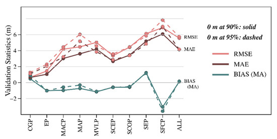
Figure 7.
Validation statistics by ecoregion and for all ecoregions combined.
3.4. The South-Wide GCHM
Figure 8 was generated using the “ALL” ecoregions regression results, extrapolated to the entire Census-based Southern Region. The figures display the recalibrated GCHMs for the 90th percentile height at 0 m height category with 80% and 20% data, in order to show the differences between simGCHM and our recalibrated GCHMs. simGCHM appeared to have much taller canopy heights than our recalibrated GCHMs. The recalibrated GCHMs with the 90th percentile height at 0 m height category with 80% and 20% data showed similar results. Figure 9 depicts the regression results obtained for each ecoregion separately. The CGP and EP are blank, due to insufficient validation data. SFCP with 20% data showed lower canopy heights. Moreover, SEP in both maps appeared homogeneous. Other ecoregions presented similar results, as shown in the figure.
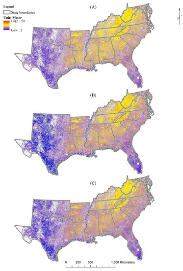
Figure 8.
The recalibrated GCHMs: (A) simGCHM, Simard et al. (2011), restricted to the southern United States; and the recalibrated GCHM using all points of 90th percentile heights at 0 m height category with (B) 80% data and (C) 20% data.
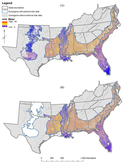
Figure 9.
The recalibrated GCHMs by each ecoregion: (A) recalibrated GCHMs of each ecoregion by 90th percentile heights at 0 m height category with 80% data and (B) 20% data.
4. Discussion
This research proceeded in three phases, centered about the second phase, recalibration. The recalibration phase assumed that a very large-scale map, such as simGCHM, must (almost by definition) have considerable small-scale prediction error. This research attempted to reduce that error, by rescaling the spatially dense map to more closely match the better quality, spatially sparse airborne lidar data. Simple linear regressions with simGCHM map heights as the predictor variables and an airborne lidar metric as the response were used to accomplish this rescaling. The simGCHM map was designed for forest canopies and, so, can be assumed to be predominantly associated with forest vegetation.
The assessment phase preceded the recalibration phase and was designed to identify a small number of potential airborne lidar response variables. A matching scheme was used, whereby four airborne lidar height categories and eight height percentiles were systematically “matched” to the simGCHM map heights. A height category includes all airborne lidar greater than a given height. It was assumed that such matching would result in a set of viable (if not optimal, in some sense) response variables. Matching was measured by MA and MAA. We found that there was a wide range of height percentiles that could be variously paired with the height categories to be used in the recalibration phase. Our research found that the 90th and 95th percentile heights (both less than maximum height) at the 0 m height category were in good agreement with simGCHM, which were chosen to advance to the recalibration phase.
The rescaling regressions were moderately successful. Short vegetation, pixels with mixed shorter and tall forest canopies, and a limited number of airborne lidar collection sites per ecoregion were the primary issues. For the most forested ecoregions, the rescaling procedure behaved as anticipated. We found that (0 m, 90th) produced the best regression results. The third (validation) phase largely corroborated the findings of the regression phase and helped to identify a leverage issue with one of the ecoregions.
When performing linear regression, ideally the “y-” (response) variables are known a priori or are chosen from a small set of variables intimately related to the purpose(s) of the study. When more than one variable suiting those purposes is available, then methods loosely classified as exploratory data analyses (EDA; after Tukey [47]) can be used (Tukey’s formal definition was more focused). With lidar point-clouds, there is so much closely related data available that ad hoc graphical or other methods are often used to assist in variable identification. That was our situation, and, thus, the first phase was exploratory, with the intent being to find the best—in some sense—response variable across ecoregions and (height percentile, minimum height category) pairs.
Overall, the shapes and levels of the individual MA curves (all panels of Figure 4) suggested a wide range of viable (airborne lidar percentiles, minimum height category) pairs for use in the recalibration phase. The differences were manifest primarily in level shifts among the ecoregions and across minimum height categories. The same can be said of the MAA curves in Figure 5. There was an apparent trade-off between height category and height percentile.
For the (0 m, 75th), height category–height percentile pair, when “averaged” across ecoregions, we saw that simGCHM predicted canopy heights on the order of eight meters taller than the airborne values, while, for the 3 m height category, the two were in good agreement across ecoregions. On the other hand, when averaged across ecoregions, the (0 m, 90th) pair showed the two measures to be in good agreement, while, for the 3 m height category, the airborne lidar values were roughly four meters larger than those of simGCHM. With the (0 m, 95th) pair, the MA curves indicated that the airborne lidar tended to overestimate the simGCHM values by about 2 m. All curves became consistently quite erratic as the height percentiles approached 100%, as expected. By erratic, we mean that the MAA values became quite large; by consistently, we mean that the simGCHM values were consistently smaller than their airborne lidar counterparts. The former has been observed in several previous studies [1,15,43,44,45,46], while the latter is probably a reflection of the fact that the large 1 km2 simGCHM pixels often partially cover non-forested areas and areas with shorter canopies.
When taken across ecoregions, the MAA curves were tightest for the 0 m height category. Over the percentile range of the 75th through the 95th, when taken across ecoregions, the MAA curves almost categorically favored the 0 m height category. Given this, and the fact that, for this height category, the range of ecosystem-specific curves clustered near MA = 0 m (i.e., best agreement), we anticipated that the (0 m, 90th) pair would perform best (on average) at the recalibration phase. We also promoted the (0 m, 95th) pair to the recalibration phase, as the 95th percentile has been suggested in several other papers. As expected, the subsequent analyses using both the 90th and 95th percentiles produced very similar results.
The MA trajectories in Figure 4 for CGP (dark blue), EP (dark green), and SFCP (orange) stood out as being either consistently above or below the others, but still having the same general shape, while those of MAP (gray) and MVLP (medium brown) were similar to each other but steeper at smaller percentile heights than those of the other ecoregions. EP had far too few observations for serious analysis.
Summarizing the Phase II recalibration results, focusing on the 90th height percentile 0 m height category after excluding simGCHM zeros and disregarding EP, we found individual values ranging from zero (SEP) to 0.75 (MVLP) and, ignoring SEP, from 0.09 (CGP) to 0.75.
Many of our previous comments have identified EP, CGP, and SFCP as being different from the other ecoregions. While the CGP has some forested areas, such as in the cross timbers regions, it is largely characterized by short crop and grassland vegetation (Table 2). The maximum 90th percentile and simGCHM heights for the CGP were 3.5 and 10 m, respectively (not on the same tree). Similarly, the SFCP had some large groves of trees, but it too is dominated by shorter vegetation, with the (mean, median) 90th percentile heights being (6.1 m, 4.1 m) when simGCHM zeros are included, and (15.5 m, 12.0 m) when they are excluded. The EP was largely ignored throughout the study, due to its paucity of data. Like the CGP and the SFCP, the EP has clusters of sizeable trees, but is largely characterized as rangeland. The two EP data values for which the simGCHM values were greater than zero had (90th, simGCHM) heights of (10.6 m, 10 m) and (7.5 m, 13 m), respectively. Coincidentally, these three ecoregions also had the three smallest sample sizes.
The SEP differed from the regions identified in the previous paragraph, in that it has extensive forest cover, comparable to MVLP. It did not stand out as particularly unusual in the assessment phase of the analysis; however, upon visual assessment of Figure 3, together with the description provided by Wiken et al. [18] (summarized in Table 2), it became apparent that this region is comprised of sub-regions with quite diverse land use and vegetation, in general ranging from tall forests in the western reaches to short vegetation interspersed with non-forest and likely diverse land use categories throughout. By inference, lefGCHM also indicates that a significant portion of the region is non-forested. Moreover, and more importantly, there were four collection sites in the region: three in Maryland, at the extreme northeast tip of the ecoregion, and one in west-central Alabama. Examination of the regression results showed that the scatter of points formed a cloud with no identifiable pattern, an intercept of about 20, and a slope and each essentially zero. From this, we concluded that it was probably the lack of spatial distribution of the airborne lidar collection sites, all apparent areas of reasonably tall canopies, and not an issue of simGCHM information over the entire extent of the region being suitable for recalibration, per se.
The remaining ecoregions achieved simGCHM > 0 m values ranging from 0.10 (MACP) to 0.75 (MAP). Examination of the associated panels of Figure 6 shows that the scatter clouds for both the MAP and MVLP exhibited what appears to be a “tail”, extending down toward the simGCHM axis. These tails were associated with shorter vegetation, with the percentile heights shorter than the simGCHM heights. These may have been the result of phenomena similar to what gave rise to that which Bolton et al. [15] noted in their comment, stating that when “the 95th height percentile was low in the Taiga Plains, Simard et al. [12] tended to estimate significantly taller canopies” (p. S144). Several of their ecozone panels exhibited this property. In their discussion, they commented further that “the RH100 metric used by Simard et al. [12] represents the tallest portion of the canopy within a 65 m GLAS footprint, whereas our estimate is the mean 95th height percentile for 25 m Lidar plots. This difference in definition likely contributed to the slight positive bias in most ecozones for the Simard et al. [12] product when compared to our airborne Lidar metric” (p. S148). While our definition of percentile height differed from that of Bolton et al.—particularly with respect to their consideration of slope and their use of forest type stratification—these comments pertain equally to our results. A related, but an alternative and rather likely, explanation is that the tails represent different sup-populations having a significant proportion of shorter woody vegetation canopies.
Except for the SFCP, our validation statistics indicated the data used for model development to be representative of the data that might be expected from other data near the same collection sites, while the results obtained for the SEP, among other concerns, point to the fact that the spatial distribution of the collection sites was an issue. The bias associated with most regions was on the order of plus-or-minus about a meter. However, for the SFCP, we found about a four-meter underestimation by simGCHM. Examination of the scatter for this region in Figure 7 revealed that this ecoregion was similar to that of the MVLP, in that it showed a clustering of values having very short airborne lidar values, which exerted a strong leverage on the fitted model (which was weak to begin with). If these values are ignored or down-weighted, the scatter reduces to a cloud with no apparent trend whatsoever.
At the large-scale, we stratified by EPA ecoregions, and the simGCHM proved to align quite well with the boundaries of those regions. At the smaller scales, our results indicated that there was likely a significant mixing of non-forested with forested area within the data. On a per-pixel basis, this can be explained by the large footprint associated with simGCHM’s reliance on RH100 data and with the large pixel size. Simard et al. [12] commented on both of these issues. simGCHM was also created using GlobeCover (another large-scale product) definitions of forests. Implicitly, as our data were aligned with simGCHM, our results were also stratified and influenced by these large-scale concerns. The strength of our results may have been improved by finer stratification; however, the sample sizes associated with the given set of airborne lidar collection sites did not permit that.
The examination of the fitted swCHM supports many of these statements. Comparing panels (A) and (B) in Figure 9, a few things stand out: first, nothing can be said for EP. Second, panel (B) indicates a general overestimation of canopy heights in CGP, MAP, MVLP, and SFCP by simGCHM, as compared to swCHM. These were precisely the ecoregions for which we identified a likely stratification issue with mixed vegetation types included in the large simGCHM pixels. Thirdly, SEP is “quite yellow” in panel (B), as compared to panel (A). This was likely an overestimation by swCHM, due to the lack of collection sites in areas representing shorter canopy heights. Perhaps the most interesting observation concerns the SCEP. This is an ecoregion that is generally forested. The two collection sites for the SCEP were in areas with mixed vegetation but, in general, more on the tall end of the canopy height spectrum. We can see that the recalibration did result in taller predictions, indicating that simGCHM may underestimate the height of taller canopies. The (0 m, 95th) results were similar, if not a bit more extreme than those of the (0 m, 90th) pair.
Our last comment concerns the finding that the fitted regression functions for all five of the ecoregions not exhibiting explained abnormalities (e.g., EP, with only two non-zero data points) passed roughly through 20 m and 20 m in Figure 6. This indicates that, at least for the ecoregions of the Southern United States, the simGCHM may be most suitable for moderately tall forested pixels. It is pixels deviating from those averages that the swCHM rescaled. The direction and magnitude of the rescaling were generally consistent with the type of vegetation of the ecoregions; however, it is apparent that the ecoregions exhibiting mixed vegetation classes might better be modeled using a finer ecoregion basis.
5. Conclusions
Our research found that the 90th and 95th percentile heights (both less than the maximum height) for the 0 m height category were in good agreement with simGCHM, and, hence, simGCHM has been appropriately developed for the height of the forest canopies in the southern United States. However, the sparseness of airborne lidar collection sites in all ecoregions was a major issue for both assessing the agreement between airborne lidar and simGCHM canopy heights and for recalibration—thus, we cannot be certain that the airborne lidar information was truly representative of canopy heights in some ecoregions. Fortunately, a significant amount of airborne lidar data is now available. Therefore, we anticipate that studies utilizing additional airborne lidar collection sites will result in better recalibration of future GCHMs.
The recalibration phase results indicated that the airborne lidar metrics were generally successful and significant variables for recalibrating simGCHM to create a more accurate product. The results also motivated us to consider more specific calibration efforts in order to improve the accuracy of GCHMs. ICESat-2 and GEDI have launched and begun collecting global vegetation data. New GCHMs are expected to be created with these data. These two sensors are expected to provide more accurate regional or global forest canopy height information than recent GCHMs. Our results should prove useful as a benchmark for future regional forest aboveground biomass estimation efforts. Furthermore, our investigations pave the way for applying the new recalibrated methodology for future GCHMs with potential applicability, using ICESat-2, GEDI, and their vegetation products.
Author Contributions
Conceptualization, N.-W.K. and S.P.; methodology, N.-W.K. and S.P.; software, N.-W.K.; validation, N.-W.K., S.P., and M.E.; formal analysis, N.-W.K., S.P., and M.E.; investigation, N.-W.K.; resources, N.-W.K.; data curation, N.-W.K.; writing—original draft preparation, N.-W.K.; writing—review and editing, M.E. and S.P.; visualization, N.-W.K. and M.E.; supervision, S.P. and M.E.; funding acquisition, S.P. All authors have read and agreed to the published version of the manuscript.
Funding
This research was partly supported by NASA’s ICESat-2 SDT (Grant #NNX15AD02G).
Institutional Review Board Statement
Not applicable.
Informed Consent Statement
Not applicable.
Data Availability Statement
Not applicable.
Acknowledgments
The authors would like to thank the Lidar Applications for the Study of Ecosystems with Remote Sensing (LASERS) Laboratory at Texas A&M University for providing airborne lidar data and software. Special thanks go to the research group of LASERS.
Conflicts of Interest
The authors declare no conflict of interest.
References
- Means, J.; Acker, S.; Fitt, B.; Renslow, M.; Emerson, L.; Hendrix, C. Predicting forest stand characteristics with airborne scanning lidar. Photogramm. Eng. Remote Sens. 2000, 66, 1367–1371. [Google Scholar]
- Popescu, S.; Wynne, R.; Nelson, R. Estimating plot-level tree heights with lidar: Local filtering with a canopy-height based variable window size. Comput. Agric. 2002, 37, 71–95. [Google Scholar] [CrossRef]
- Lefsky, M.; Harding, D.; Keller, M.; Cohen, W.; Carabajal, C.; del Bom Espirito-Santo, F.; de Oliveira, R., Jr. Estimates of forest canopy height and aboveground biomass using ICESat. Geophys. Res. Lett. 2005, 32, L22S02, Erratum in Lefsky, M.; Harding, D.; Keller, M.; Cohen, W.; Carabajal, C.; del Bom Espirito-Santo, F.; de Camargo, P. Correction to “Estimates of forest canopy height and aboveground biomass using ICESat’’. Geophys. Res. Lett. 2006, 32, L05501. [Google Scholar] [CrossRef]
- Mustonen, J.; Packalén, P.; Kangas, A. Automatic segmentation of forest stands using a canopy height model and aerial photography. Scand. J. For. Res. 2008, 23, 534–545. [Google Scholar] [CrossRef]
- Fayad, I.; Baghdadi, N.; Bailly, J.S.; Barbier, N.; Gond, V.; Hérault, B.; El Hajj, M.; Fabre, F.; Perrin, J. Regional scale rain-forest height mapping using regression-kriging of spaceborne and airborne LiDAR data: Application on French Guiana. Remote Sens. 2016, 8, 240. [Google Scholar] [CrossRef]
- Ni, X.; Zhou, Y.; Cao, C.; Wang, X.; Shi, Y.; Park, T.; Choi, S.; Myneni, R.B. Mapping forest canopy height over continental China using multi-source remote sensing data. Remote Sens. 2015, 7, 8436–8452. [Google Scholar] [CrossRef]
- Ni, X.; Park, T.; Choi, S.; Shi, Y.; Cao, C.; Wang, X.; Lefsky, M.A.; Simard, M.; Myneni, R.B. Allometric scaling and resource limitations model of tree heights: Part 3. Model optimization and testing over continental China. Remote Sens. 2014, 6, 3533–3553. [Google Scholar] [CrossRef]
- Shi, Y.; Choi, S.; Ni, X.; Ganguly, S.; Zhang, G.; Duong, H.V.; Lefsky, M.A.; Simard, M.; Saatchi, S.S.; Lee, S.; et al. Allometric scaling and resource limitations model of tree heights: Part 1. Model optimization and testing over continental USA. Remote Sens. 2013, 5, 284–306. [Google Scholar] [CrossRef]
- Popescu, S.; Zhou, T.; Nelson, R.; Neuenschwander, A.; Sheridan, R.; Narine, L.; Walsh, K. Photon counting LiDAR: An adaptive ground and canopy height retrieval algorithm for ICESat-2 data. Remote Sens. Environ. 2018, 208, 154–170. [Google Scholar] [CrossRef]
- Narine, L.; Popescu, S.; Neuenschwander, A.; Zhou, T.; Srinivasan, S.; Harbeck, K. Estimating aboveground biomass and forest canopy cover with simulated ICESat-2 data. Remote Sens. Environ. 2019, 224, 1–11. [Google Scholar] [CrossRef]
- Lefsky, M. A global forest canopy height map from the Moderate Resolution Imaging Spectroradiometer and the Geoscience Laser Altimeter System. Geophys. Res. Lett. 2010, 37. [Google Scholar] [CrossRef]
- Simard, M.; Pinto, N.; Fisher, J.; Baccini, A. Mapping forest canopy height globally with spaceborne lidar. J. Geophys. Res. 2011, 116. [Google Scholar] [CrossRef]
- Los, S.; Rosette, J.; Kljun, N.; North, P.; Chasmer, L.; Suárez, J.; Berni, J. Vegetation height and cover fraction between 60° S and 60° N from ICESat GLAS data. Geosci. Model Dev. 2012, 5, 413–432. [Google Scholar] [CrossRef]
- Wang, Y.; Li, G.; Ding, J.; Guo, Z.; Tang, S.; Wang, C.; Huang, Q.; Liu, R.; Chen, J.M. A combined GLAS and MODIS estimation of the global distribution of mean forest canopy height. Remote Sens. Environ. 2016, 174, 24–43. [Google Scholar] [CrossRef]
- Bolton, D.; Coops, N.; Wulder, M. Investigating the agreement between global canopy height maps and airborne Lidar derived height estimates over Canada. Can. J. Remote Sens. 2013, 39, 139–151. [Google Scholar] [CrossRef]
- Census Regions and Divisions of the United States. Available online: https://www2.census.gov/geo/pdfs/maps-data/maps/reference/us_regdiv.pdf (accessed on 20 December 2019).
- Köppen, W.; Volken, E.; Brönnimann, S. The thermal zones of the earth according to the duration of hot, moderate and cold periods and to the impact of heat on the organic world . Meteorol. Z. 2011, 20, 351–360, (Translated from: Die Wärmezonen der Erde, nach der Dauer der heissen, gemässigten und kalten Zeit und nach der Wirkung der Wärme auf die organische Welt betrachtet. Meteorol. Z. 1884, 1, 215–226). [Google Scholar]
- Wiken, E.; Nava, F.; Griffith, G. North American Terrestrial Ecoregions-Level III. Technical; Commission for Environmental Cooperation: Montreal, QC, Canada, 2011. [Google Scholar]
- Omernik, J.; Griffith, G. Ecoregions of the Conterminous United States: Evolution of a Hierarchical Spatial Framework. Environ. Manag. 2014, 54, 1249–1266. [Google Scholar] [CrossRef] [PubMed]
- Ecoregions|Ecosystem Research|US EPA. Available online: https://www.epa.gov/eco-research/ecoregions (accessed on 20 December 2019).
- Saatchi, S.S.; Harris, N.L.; Brown, S.; Lefsky, M.; Mitchard, E.T.; Salas, W.; Zutta, B.R.; Buermann, W.; Lewis, S.L.; Hagen, S.; et al. Benchmark map of forest carbon stocks in tropical regions across three continents. Proc. Natl. Acad. Sci. USA 2011, 108, 9899–9904. [Google Scholar] [CrossRef]
- Harding, D.; Carabajal, C. ICESat waveform measurements of within-footprint topographic relief and vegetation vertical structure. Geophys. Res. Lett. 2005, 32. [Google Scholar] [CrossRef]
- Boudreau, J.; Nelson, R.; Margolis, H.; Beaudoin, A.; Guindon, L.; Kimes, D. Regional aboveground forest biomass using airborne and spaceborne LiDAR in Québec. Remote Sens. Environ. 2008, 112, 3876–3890. [Google Scholar] [CrossRef]
- Sun, G.; Ranson, K.; Kimes, D.; Blair, J.; Kovacs, K. Forest vertical structure from GLAS: An evaluation using LVIS and SRTM data. Remote Sens. Environ. 2008, 112, 107–117. [Google Scholar] [CrossRef]
- Kummerow, C.; Barnes, W.; Kozu, T.; Shiue, J.; Simpson, J. The Tropical Rainfall Measuring Mission (TRMM) sensor package. J. Atmos. Ocean. Technol. 1998, 15, 809–817. [Google Scholar] [CrossRef]
- Hijmans, R.; Cameron, S.; Parra, J.; Jones, P.; Jarvis, A. Very high resolution interpolated climate surfaces for global land areas. Int. J. Climatol. 2005, 25, 1965–1978. [Google Scholar] [CrossRef]
- Farr, T.; Rosen, P.; Caro, E.; Crippen, R.; Duren, R.; Hensley, S.; Alsdorf, D. The Shuttle Radar Topography Mission. Rev. Geophys. 2007, 45, 1–33. [Google Scholar] [CrossRef]
- USGS. Shuttle Radar Topography Mission, 30 Arc Second Product, Version 2.0. Technical; Global Land Cover Facility; University of Maryland: College Park, MD, USA, 2006.
- Hansen, M.; DeFries, R.; Townshend, J.; Carroll, M.; Dimiceli, C.; Sohlberg, R. Global percent tree cover at a spatial resolution of 500 meters: First results of the MODIS vegetation continuous fields algorithm. Earth Interact. 2003, 7, 1–15. [Google Scholar] [CrossRef]
- Hagolle, O.; Lobo, A.; Maisongrande, P.; Cabot, F.; Duchemin, B.; De Pereyra, A. Quality assessment and improvement of temporally composited products of remotely sensed imagery by combination of VEGETATION 1 and 2 images. Remote Sens. Environ. 2005, 94, 172–186. [Google Scholar] [CrossRef]
- Breiman, L. Random forests. Mach. Learn. 2001, 45, 5–32. [Google Scholar] [CrossRef]
- Liaw, A.; Wiener, M. Classification and Regression by randomForest. R News 2002, 2, 18–22. [Google Scholar]
- Baldocchi, D.; Falge, E.; Gu, L.; Olson, R.; Hollinger, D.; Running, S.; Wofsy, S. FLUXNET: A new tool to study the temporal and spatial variability of ecosystem-scale carbon dioxide, water vapor, and energy flux densities. Bull. Am. Meteorol. Soc. 2001, 82, 2415–2434. [Google Scholar] [CrossRef]
- Baldocchi, D. ‘Breathing’ of the terrestrial biosphere: Lessons learned from a global network of carbon dioxide flux measurement systems. Aust. J. Bot. 2008, 56, 1–26. [Google Scholar] [CrossRef]
- Bevan, S.; Los, S.; North, P. Response of vegetation to the 2003 European drought was mitigated by height. Biogeosciences 2014, 11, 2897–2908. [Google Scholar] [CrossRef]
- Rosette, J.; North, P.; Suárez, J. Vegetation height estimates for a mixed temperate forest using satellite laser altimetry. Int. J. Remote Sens. 2008, 29, 1475–1493. [Google Scholar] [CrossRef]
- Global 1 km Forest Canopy Height (Simard et al., 2011). Available online: https://webmap.ornl.gov/wcsdown/dataset.jsp?ds_id=10023 (accessed on 20 December 2019).
- G-LiHT. Available online: https://gliht.gsfc.nasa.gov/ (accessed on 20 December 2019).
- Airborne Remote Sensing|NSF NEON|Open Data to Understand our Ecosystems. Available online: https://www.neonscience.org/data-collection/airborne-remote-sensing (accessed on 20 December 2019).
- Home|OpenTopography. Available online: https://opentopography.org/ (accessed on 20 December 2019).
- Hodgson, M.; Jensen, J.; Schmidt, L.; Schill, S.; Davis, B. An evaluation of LIDAR- and IFSAR-derived digital elevation models in leaf-on conditions with USGS Level 1 and Level 2 DEMs. Remote Sens. Environ. 2003, 84, 295–308. [Google Scholar] [CrossRef]
- Wulder, M.; White, J.; Bater, C.; Coops, N.; Hopkins, C.; Chen, G. Lidar plots-a new large-area data collection option: Context, concepts, and case study. Can. J. Remote Sens. 2012, 38, 600–618. [Google Scholar] [CrossRef]
- Drake, J.; Dubayah, R.; Knox, R.; Clark, D.; Blair, J. Sensitivity of large-footprint lidar to canopy structure and biomass in a neotropical rainforest. Remote Sens. Environ. 2002, 81, 378–392. [Google Scholar] [CrossRef]
- St-Onge, B.; Vega, C.; Fournier, R.; Hu, Y. Mapping canopy height using a combination of digital stereo-photogrammetry and lidar. Int. J. Remote Sens. 2008, 29, 3343–3364. [Google Scholar] [CrossRef]
- Kane, V.; McGaughey, R.; Bakker, J.; Gersonde, R.; Lutz, J.; Franklin, J. Comparisons between field- and LiDAR-based measures of stand structural complexity. Can. J. For. Res. 2010, 40, 761–773. [Google Scholar] [CrossRef]
- Alexander, C.; Bøcher, P.; Arge, L.; Svenning, J.-C. Regional-scale mapping of tree cover, height and main phenological tree types using airborne laser scanning data. Remote Sens. Environ. 2014, 147, 156–172. [Google Scholar] [CrossRef]
- Tukey, J.W. Exploratory Data Analysis; Addison-Wesley Publishing Company: Boston, MA, USA, 1977. [Google Scholar]


Publisher’s Note: MDPI stays neutral with regard to jurisdictional claims in published maps and institutional affiliations. |
© 2021 by the authors. Licensee MDPI, Basel, Switzerland. This article is an open access article distributed under the terms and conditions of the Creative Commons Attribution (CC BY) license (https://creativecommons.org/licenses/by/4.0/).