Land Cover-Specific Local Incidence Angle Correction: A Method for Time-Series Analysis of Forest Ecosystems

Abstract

This study deals with a local incidence angle correction method, i.e., the land cover-specific local incidence angle correction (LC-SLIAC), based on the linear relationship between the backscatter values and the local incidence angle (LIA) for a given land cover type in the monitored area. Using the combination of CORINE Land Cover and Hansen et al.’s Global Forest Change databases, a wide range of different LIAs for a specific forest type can be generated for each scene. The algorithm was developed and tested in the cloud-based platform Google Earth Engine (GEE) using Sentinel-1 open access data, Shuttle Radar Topography Mission (SRTM) digital elevation model, and CORINE Land Cover and Hansen et al.’s Global Forest Change databases. The developed method was created primarily for time-series analyses of forests in mountainous areas. LC-SLIAC was tested in 16 study areas over several protected areas in Central Europe. The results after correction by LC-SLIAC showed a reduction of variance and range of backscatter values. Statistically significant reduction in variance (of more than 40%) was achieved in areas with LIA range >50° and LIA interquartile range (IQR) >12°, while in areas with low LIA range and LIA IQR, the decrease in variance was very low and statistically not significant. Six case studies with different LIA ranges were further analyzed in pre- and post-correction time series. Time-series after the correction showed a reduced fluctuation of backscatter values caused by different LIAs in each acquisition path. This reduction was statistically significant (with up to 95% reduction of variance) in areas with a difference in LIA greater than or equal to 27°. LC-SLIAC is freely available on GitHub and GEE, making the method accessible to the wide remote sensing community.

1. Introduction

In the field of remote sensing, the 21st century is referred to as “the era of big data”, in which a large amount of (not only) freely available data is accessible. When processing a large amount of data, especially for time series analysis, it is productive to use tools that can process them quickly and effectively. In some cases, there may be time and performance issues and limitations using traditional desktop solutions, where it is necessary to download and preprocess data before the necessary analyses can be performed on them. As a consequence, the so-called cloud platforms have been developed. They store not only images and data archives, but they also bring the computing technology needed for data processing [1,2].

In forest monitoring, multispectral optical satellite data have proven to be a very effective data source. In many cases, however, optical data have certain shortcomings, especially regarding the presence of clouds. Electromagnetic waves in the microwave spectrum can penetrate clouds, fog and light rain and are not dependent on sunlight. Therefore, sensors in these wavelengths can observe the Earth’s surface both during the day and at night. Additionally, they can be potentially used in monitoring landscape changes as complementary to optical data (i.e., in [3]). Since the launch of the Sentinel-1 satellite in 2014, providing freely available synthetic aperture radar (SAR) data in C-band, interest in SAR data has started to grow, and new methods began to be developed. Systematic sensing of the Earth’s surface with constant geometric characteristics of the sensors brought many advantages over previous radar missions.

The interaction between the SAR signal and the surface depends mainly on the characteristics of the studied object, e.g., on the shape, roughness and dielectric properties (mainly moisture) [4], as well as on the sensor characteristics, i.e., on wavelength, incidence angle and polarization [5,6,7,8]. Characteristics of the studied object are different for every land cover class and can be biased by some environmental factors, like moisture content [9], change in temperature [10,11], etc. The radar incidence angle is increasing from near range to far range, which causes variations of the backscatter values for a given land cover class, resulting in different backscatter for the same class at different incidence angles. The correction of the radar incidence angle can be only valid in ideal situations, where the effect of terrain can be neglected, e.g., over relatively flat areas (e.g., in [12]) or over the sea (e.g., in [13]). On the other hand, in the case of areas with rugged terrain, the incidence angle of the electromagnetic wave is affected by the slope and aspect of the studied terrain. Thus, the effect of the terrain needs to be considered and eliminated or at least minimized for appropriate evaluation and interpretation of obtained backscatter. This factor is most apparent in the intensity of the received signal in the case of a combination of images from different orbits and paths of the satellite (ascending vs. descending or adjacent paths covering a given area). Analysis in mountainous areas, where the slope and orientation of the terrain are not considered, i.e., only flat Earth approximations are used, leads to errors [14]. This is especially important for forests, as most of the forests of Central Europe are located in mountainous areas, particularly national parks and protected areas. In the time-series analysis, this effect is a constant fluctuation of the backscatter values acquired from different successive paths. To ensure the highest possible temporal resolution of satellite data in the time-series analysis, it is necessary to use all available acquisition orbits and paths of an observed area. Therefore, to obtain accurate information in the time-series analysis that represents a real status or change over an area, it is necessary to eliminate the influence of the terrain.

There are several techniques to correct the topographic effects. As per the relevant literature, the first approaches used to correct the topographic effect belong to methods based on cosine square correction [13,15,16,17,18]. Currently, the most used and well-known algorithm for correcting the topographic effect is the Radiometric Terrain Correction developed by Small [19] available for desktop software, such as SNAP Sentinel-1 Toolbox. Using this method, not only the geometry but also the radiometry of the scene is corrected for the terrain influences [7]. In this method, accurate knowledge of the acquisition geometry of the image and a DEM are used to estimate the local illuminated area of each image pixel [19]. A local illuminated area is then used to normalize the backscatter value.

In some recent studies, in the process of removing the backscatter dependency on the radar incidence angle or on the local incidence angle (LIA), so-called regression-based normalizations were used, where all image pixels are corrected to the same reference incidence angle (e.g., in [20,21,22,23]). The prerequisite for successful application of the regression-based normalization is to find the relationship between the backscatter and incidence angle, therefore, to obtain the slope coefficient of the regression line. The regression-based normalization is used mainly for the so-called pixel-based method, where the slope coefficient is calculated for each image pixel separately, using several satellite images from the specified time range (e.g., in [20,21,23,24,25]). As the pixel-based method can be computationally intensive for large areas, Widhalm et al. [26] developed the so-called slope approach, aiming to normalize the backscatter–LIA dependence using only single images. In that approach, the slope coefficients of the linear regression were determined for each land cover type separately, based on which they created specific coefficients used in the further regression-based normalization, which are valid only for specific high latitude areas. However, they found that their approach is not suitable for applications in mountainous areas, as the linear relationship between backscatter and LIA was not valid. Nonlinear relationship over sloped terrain was also found in [27] and stated in [12].

In exploring backscatter–LIA dependence, it is important to note that different land cover types have a different backscatter–LIA relationship, as found in previous studies [16,26,28,29]. Hinse et al. [16] found a flat angular behavior over deciduous and coniferous forests (0.01 and 0.02 dB/degree, respectively) and steeper in agricultural lands and cornfields (0.15 and 0.11 dB/degree, respectively). In [28,29], the backscatter–LIA dependence was compared for the tropical forest, tree savannah, Sahelian area and desert classes. In this case, tropical forest areas had a flatter angular behavior (0.06 dB/degree) than other land cover types. Widhalm et al. [26] calculated the regression slope coefficients of the backscatter–LIA dependence for 56 sample classes, in which values were in the range from 0.07 to 0.3 dB/degree, while forests had values from 0.07 to 0.17 dB/degree.

A modern method in the processing of RS data is cloud computing. The most popular cloud-based platform has become Google Earth Engine (GEE), with a rapid yearly increase in usage for a wide range of applications [1]. GEE (https://earthengine.google.com, last accessed 26 April 2021) contains “multi-petabyte” analysis-ready data, in combination with all computation power located in the cloud. It can be accessed through an Internet-accessible application programming interface (API) and a web-based interactive development environment (IDE). Therefore, users can access data and perform analysis through any web browser. It is freely accessible for research, education and nonprofit use [2]. If radar satellite data are used in GEE, there are limited options for correcting topographic effects. Vollrath et al. [30] published a method to eliminate the effects of the terrain on radar satellite data in the GEE environment. That methodology is based on using two physical reference models used to correct the backscattering behavior. The first model is developed for vegetation monitoring, where volume scattering is the dominant scattering type, and the second one is developed for areas with surface scattering. However, the effect of different backscatter–LIA relationships for specific land cover classes is not reflected in this method.

The presented study introduces a land cover-specific correction of the local incidence angle using linear regression analysis in GEE. This method is called the land cover-specific local incidence angle correction (LC-SLIAC). The land cover-specific method of the LC-SLIAC aims to correct one specific land cover class, i.e., in the case of this study, to correct backscatter over forests. The purpose of the LC-SLIAC method is based on previous studies, where different backscatter–LIA relationships were proved for different land cover classes (e.g., [16,26,28,29]). Using this algorithm, the terrain effects of each individual scene and in the time-series curve are eliminated. The method’s suitability was tested on time series of coniferous and deciduous forests in selected areas in Central Europe. The main difference between most of the above-mentioned regression-based normalization approaches and LC-SLIAC is in using a single image to calculate the dependence of backscatter values of a selected forest type on LIA. This is possible using available land cover databases containing information on the spatial distribution of a given land cover type. Therefore, for each SAR scene, it is possible to calculate the backscatter–LIA dependency separately. The next methodological aspect is using the site- and path-specific reference incidence angles for time-series analysis.

In this context, the main aim of the study is to introduce the LC-SLIAC method and to test its suitability for eliminating the effect of the terrain. The accuracy of the proposed method is tested by statistical evaluation and comparison of backscatter of forest areas before and after the correction for forests with different characteristics—at a different elevation, terrain slope and orientation, and with different characteristics of the LIA. Moreover, the effectiveness of the method is tested within a three-month time-series analysis of coniferous and deciduous forests.

2. Materials and Methods

2.1. Study Areas

The selection of study areas (SA) was limited to four Central European countries—Czechia, Slovakia, Hungary and Poland (Figure 1). A total of 16 study areas—8 with a majority of coniferous forests and 8 with a majority of deciduous forests—were selected. Each SA was defined as a 20 × 20 km bounding box around a central point. The main criterion for selecting the SA was that the share of forests (according to the forest mask) must be higher than 40%. An exception was given to SA16 with only a 22% share of forests. In similar 20 × 20 km areas located in lowlands of Central Europe with a mean elevation of 150 m a.s.l., the share of forests is usually very low—most of the areas are represented by agricultural lands. Another criterion for the selected areas was to be characterized by a majority of coniferous or deciduous forests in different national parks (NP) or protected landscape areas (PLA) at various elevations and with different slope values (

Table 1. Characteristics of study areas.

Study Area	Coordinates of the Central Point (x, y)	Mean Elevation (m a.s.l.)	Mean Slope (°)	Share of Forest Areas (%)	Description
1	15.6930, 50.7245	924.4	14.6	45.4	Coniferous forest in the Krkonoše NP (CZ/PL)
2	22.4457, 50.6717	223.7	2.7	42.0	Coniferous forest in Lasy Janowskie PLA (PL)
3	17.2847, 50.1419	839.2	13.3	53.5	Coniferous forest in Jeseníky PLA (CZ)
4	16.0196, 49.6786	679.2	5.7	47.5	Coniferous forest in Žďárské vrchy PLA (CZ)
5	18.5186, 49.4805	722.4	15.3	60.5	Coniferous forest in Beskydy PLA (CZ/SK)
6	19.7257, 49.2604	1168.9	18.7	40.2	Coniferous forest in the High Tatras NP (SK/PL)
7	14.8375, 48.9250	468.9	3.7	40.3	Coniferous forest in Třeboňsko PLA (CZ)
8	20.0088, 48.9569	1098.3	18.4	42.0	Coniferous forest in the Low Tatras NP (SK)
9 *	22.5540, 49.1913	752.5	14.2	47.3	Broadleaf forest in Bieszczady NP (PL)
10 *	22.2175, 48.8988	471.2	10.9	64.0	Broadleaf forest in Vihorlat PLA (SK)
11 *	17.2490, 48.3916	357.7	9.1	55.0	Broadleaf forest in Malé Karpáty PLA (SK)
12 *	18.7857, 48.4121	510.3	13.8	48.5	Broadleaf forest in Štiavnické vrchy PLA (SK)
13 *	21.4618, 48.4200	334.7	11.6	58.7	Broadleaf forest in Zemplén mountains PLA (HU)
14 *	20.5455, 48.0475	515.1	13.6	75.2	Broadleaf forest in Bükk NP (HU)
15 *	18.9683, 47.7215	276.7	9.3	47.6	Broadleaf forest in Duna-Ipoly-NP (HU)
16 *	21.9982, 47.6490	150.2	2.7	22.0	Broadleaf forest in Hajdúsági PLA (HU)

* study area with majority of deciduous forests.

). Selected SAs can be divided into three main categories according to the mean slope: 1) SAs with gentle slopes of 2–6° (SA2, SA4, SA7 and SA16), with a moderate slope of 9–15° (SA1, SA3–SA5, SA9–15) and with steep slopes of higher than 18° (SA6 and SA8).

For further testing of the effectiveness of the proposed method on short-term time series, six central points of study areas were selected. A 20 m buffer was created around these points (hereafter referred to as case study—CS). Three case studies represent three coniferous (CS5, CS7 and CS8) and three deciduous forest examples (CS9, CS11 and CS13), with three different types of LIA ranges—very high, moderate and very low. The main criterion in selecting these case studies was that these areas had to be stable—not disturbed by anthropogenic or environmental factors in the time range 2015–2020. For these case studies, various characteristics were calculated—elevation, slope and aspect values and LIA range with minimum and maximum values (

Table 2. Characteristics of case studies for use in the short-term time-series analysis.

Case Study	Coordinates (x, y)	Elevation (m a.s.l.)	Slope/Aspect (Degrees)	LIA Range (Max–Min) in Degrees
5	16.0196, 49.6786	707	19/86	40 (57–17)
7	18.5186, 49.4805	480	1/105	10 (41–31)
8	22.4457, 50.6717	1106	31/250	69 (72–3)
9 *	18.7857, 48.4121	708	25/308	27 (66–39)
11 *	22.2175, 48.8988	556	7/32	4 (43–39)
13 *	20.5455, 48.0475	365	31/97	60 (69–9)

* case study represented by deciduous forests.

).

2.2. Data

The main data source for this study was Sentinel-1 SAR data. Sentinel-1 satellite family represents the continuation of earlier C-band spaceborne radar sensors of the ERS-1, ERS-2 and Envisat/ASAR missions of the European Space Agency (ESA). The Sentinel-1 is the first series designed to meet the requirements of the earth observation of the European Union (EU). The Sentinel-1 mission comprises a constellation of two satellites, Sentinel-1A and Sentinel-1B, sharing the same orbital plane. Satellites operate at C-band, at the center frequency of 5.405 GHz, orbiting in a near-polar sun-synchronous orbit at the height of 693 km, having a 12-day repeat cycle per satellite. Preprocessed Level-1 data include two categories: Single Look Complex imagery (SLC) is used mainly for interferometric applications, and Ground Range Detected georeferenced (GRD) imagery for intensity-based applications [31]. In this study, Sentinel-1 level-1 GRD scenes were used, which are available in GEE, where they were preprocessed. Preprocessing of scenes in GEE was performed using the SNAP Sentinel-1 toolbox and includes the following steps: applying the orbit file, GRD border noise removal, thermal noise removal, radiometric calibration, terrain correction (orthorectification) using the SRTM 30-m DEM or the ASTER DEM for high latitudes (>60° or <−60°). The most used method for correction of terrain effects on backscatter values, the Radiometric Terrain Correction [19], was not applied in GEE due to artifacts on mountain slopes [32].

Another important input data in the presented study was the Shuttle Radar Topography Mission digital elevation model (SRTM DEM), which was created based on the need for globally consistent topographic data using an established mapping technique, i.e., SAR interferometry (InSAR). As the data acquisition was done using radar, the signal’s return could be influenced by vegetation, especially by its height, structure and density [33]. The database in GEE (SRTM V3 product/SRTM Plus provided by NASA JPL), in contrast to earlier versions, undergoes a void-filling process using open-source datasets, such as ASTER GDEM2 GMTED2010 and NED [34]. Data are available in 1 arc-second resolution, which corresponds to an area of approximately 30 × 20 m at Central Europe latitudes (approx. 50°). According to the accuracy assessment, the data achieved a height accuracy from 7 to 13 m depending on the continent, e.g., for Eurasia, it was 8.8 m [33].

In this study, two land cover databases were used as complementary data: the CORINE Land Cover (CLC) and Hansen et al.’s Global Forest Change (GFC) databases available in GEE. CLC is a land cover inventory initiated in 1985, including five subsequent databases (CLC1990, CLC2000, CLC2006, CLC2012 and the latest CLC2018). The datasets were created by classifying satellite images with in situ measurements used as ancillary data at a national level by national teams coordinated by the European Environment Agency (EEA). All CLC databases have the same definition of main technical parameters: the minimum mapping unit (MMU) was set to 25 hectares, the minimum width of a linear element (MMW) to 100 m and the database nomenclature includes 44 land cover classes grouped in a three-level hierarchy [35]. These datasets are available in GEE in a 100 × 100 m grid. In this study, the CLC2018 product was used. According to the CLC2018 nomenclature, deciduous forest belongs to the category 311, coniferous forest to 312 and mixed forest to 313. In these categories, only trees higher than 5 m were taken into consideration with at least 30% forest crown cover. Based on their definition, the coniferous forest class includes areas where coniferous forests represent at least 75% of the formation. The same was applied to the deciduous forest, where 75% of trees must belong to deciduous stands [36]. From both types of forest class definitions, the mixed-forest areas were excluded, while this class is defined separately in the database.

The GFC represents a database of global tree cover extent, loss and gain at a spatial resolution of 30 m, originally created for the period from 2000 to 2012 [37], later accompanied by data from subsequent years. Trees were defined in this database as all vegetation taller than 5 m in height, which matches the minimum tree height definition in CLC. Forest loss was defined as a change of forest stand, having at least 50% of crown cover at Landsat pixel scale to non-forest (~0% crown cover), while forest gain represents the inverse situation, where the non-forest state changes to the forest. In this study, the 1.6 version of the database was used, including global forest cover to 2018. Several changes were done relative to the original 1.0 version from 2013: Landsat 8 OLI data were used; reprocessing of forest loss was done from 2011; the training data calibration; and the input spectral features for the loss model were improved [38].

For accuracy assessment of the forest mask in each study area, national orthophoto images were primarily used combined with Google Earth Pro images (CNES/Airbus; Landsat/Copernicus; Maxar Technologies; Eurosens/Geodis Slovakia) from the period 2017–2019. In Czechia, national orthophoto images from 2017 and 2019 (western part of Czechia) and 2018 (eastern part of Czechia) from the Czech Office for Surveying, Mapping and Cadastre (ČÚZK) were used. For SAs located in Slovakia, orthophotos from 2017 (western part of Slovakia), 2018 (center part) and 2019 (eastern part) were used from the office of Geodesy, Cartography and Cadastre Authority of the Slovak Republic (ÚGKK SR). Forest areas located in areas covered by images from 2017 were further checked using Google Earth Pro images. For SAs in Poland, orthophotos from 2019 from the Head Office of Geodesy and Cartography were used. For Hungarian SAs, only Google Earth Pro images were available.

2.3. Methodology

The most important step in the LC-SLIAC methodology was to calculate the LIA for every image pixel, while it was necessary to calculate other parameters from the DEM (slope and aspect) and SAR images (viewing azimuth). For SAR images, the active shadow and layover areas were masked out, followed by the generation of the forest mask and its validation, which was used to select an appropriate number of forest areas in each of the 16 SAs to explain the relationship between LIA and backscatter in the linear regression analysis. These relationships in SAs were evaluated and statistically compared with each other. The correction itself was then done for each image separately. Results after correction were evaluated and compared to non-corrected data for each SA. In the final step, three-month time series were created for six case studies and statistics before and after the correction were compared. Figure 2 shows the workflow of the methodology. The following paragraphs explain in detail each step.

LIA is the angle between the look (incidence) vector i and the vector n normal to the surface [16,39,40,41], as illustrated in Figure 3. The derivation of the equation for the calculation of LIA (Equation (1)) is based on a calculation of the angle between the incidence vector i and the normal to the surface n (available in [42]). The calculation of the LIA requires knowledge of the slope α and aspect angles β of the examined area and the viewing azimuth of the sensor γ (Figure 4). After the derivation, the following equation is applicable for the calculation of LIA:

cosθ₀ = cosθ ∗ cosα + sinα ∗ sinθ ∗ cos(γ’ − β),

(1)

where θ₀ is the LIA, θ is the radar incidence angle, α is the local slope, β is the aspect angle of the terrain and γ is the viewing angle and γ’ = γ − 180°. γ’ is used in Equation (1), as it is assumed that vectors i and n have the same direction, having the same initial point A (Figure 4). For this reason, there is a need to subtract 180° from the viewing angle γ to get that direction of the vector i. The following Equation (2), where the original direction of the incidence wave is considered (as in [39]), was used to calculate the LIA for every image pixel:

cosθ₀ = cosθ ∗ cosα − sinα ∗ sinθ ∗ cos(γ − β).

(2)

The calculation of LIA using Equation (2) requires the terrain slope α and aspect angles β, viewing azimuth of the sensor γ and radar incidence angle θ values for each pixel. Radar incidence angle θ is known for each pixel, as it is available as a separate band in the Sentinel-1 GRD product. Slope and aspect angles for each pixel were generated from SRTM DEM and then projected and resampled by the nearest neighbor method to the Sentinel-1 band’s projection and resolution grid, respectively. The viewing azimuth γ is perpendicular to the flight direction azimuth of the satellite respective to the true north N. The flight azimuth was derived by determining the corner points of the near range of the image, representing points lying on the vector parallel to the flight direction vector, according to [43] (for more details see [42]). The viewing azimuth γ and the LIA calculations were performed for each image separately, as the ascending and descending passes have different viewing azimuths.

Radiometric distortions caused by the side-looking geometry of the radar (radar shadow and layover), having increased occurrence in mountainous areas, were removed in the next step. A simplified method presented in [30] was used for shadow and layover masking for each image separately. Only pixels lying in an active layover and shadow regions were considered. The formulas to generate these regions, originally presented in [44], are the following:

active layover = α_r > θ,

(3)

active shadow = α_r < − (90° − θ),

(4)

where θ is the radar incidence angle and α_r is the slope in the range defined as:

α_r = arctan(tan(β) ∗ cos(Φ)),

(5)

where Φ is the difference between the viewing azimuth of the sensor γ and the slope α given by Φ = γ − α. From the preprocessed Sentinel-1 GRD data, it is not possible to reconstruct the passive shadow and layover regions. As an alternative solution for computing the passive regions, a buffer was created around each found active layover and shadow image pixel as in [30]. In the case of this study, it was a 20 m buffer. The resulting layover and shadow masks were merged and applied to each Sentinel-1 image. Masked ascending and descending image databases were then merged into one dataset.

The forest mask was then generated using the combination of CLC2018 and GFC databases. The base layer from 2000 of the GFC was used, where only forest pixels with crown cover >50% were selected in this study. After this, pixels corresponding to the forest loss from 2000 to 2018 were masked out from the base layer. The resulting layer was overlaid with a selected forest class layer of the CLC2018, resulting in a final forest mask. As a result, two forest mask layers were available—deciduous and coniferous forest mask. For these forest masks, an accuracy assessment was performed in each study area. In the first step, 600 randomly selected points were generated in the areas of the forest masks within the SAs. A 20 m buffer was generated around these points, and areas lying completely within the forest mask were then selected (hereafter referred to as “forest areas”). A total of 1099 control areas were used (540 for coniferous forest and 559 for deciduous forest mask). National orthophotos and images from Google Earth Pro were used as ground truth data. For the purposes of accuracy assessment, three categories were defined: (1) forest areas with more than 75% crown cover in the forest area, (2) forest areas with less than 75% crown cover, and (3) forest areas representing the opposite forest category, i.e., coniferous forest in case of assessment of deciduous forest areas. Inspired by the CLC nomenclature [35], forest areas corresponding to category (1) were considered to be correctly defined forest areas and areas corresponding to categories (2) and (3) to be incorrectly defined forest areas (errors). The accuracy assessment of the forest mask for each SA and the overall accuracy for the entire forest mask was calculated.

After the accuracy assessment was calculated, one thousand random points were then generated, and a 20 m buffer was created around these points in each study area to collect an adequate amount of data to perform a linear regression analysis. Areas lying completely inside the created forest mask were selected for further analysis (forest areas), ensuring that only forest areas will serve as input data to the regression analysis. These forest areas were overlaid with Sentinel-1 images, and the mean values of backscatter and LIA were extracted from its areas to ensure the reduction of the speckle effect. Forest areas representing outliers for backscatter values were excluded using Tukey’s fences—using lower and upper fences—in each polarization separately. The least-squares estimate of a linear function of one variable with a constant term was then calculated from the selected forest areas using the following equation:

σ_est = a + b ∗ θ₀

(6)

where σ_est represents the estimated value of the backscatter (σ⁰), θ₀ is LIA, a and b are the offset and slope coefficients of the regression line, respectively.

The generation of forest areas and the subsequent calculation of the offset and slope coefficients of the linear regression line were performed separately for each image in the selected time and spatial range. These values were saved as image properties for the next computations. To statistically test and compare the relationship between LIA and backscatter values in each SA, statistics were calculated for the selected forest areas (mean elevation, LIA range, LIA interquartile range (LIA IQR)) and the values of linear regression line slope (coefficient b), R², p-value and RMSE for both polarizations were derived from all available images. These statistics were first calculated for each image separately in the time range of June–August 2018, and then the mean was calculated from this time range and used in the comparison. To determine which characteristic of SAs’ forest areas (LIA IQR, LIA range, and mean elevation) has the biggest effect on statistical parameters (RMSE, R²) and on the scale coefficient b, a pair-wise correlation was performed to calculate Pearson’s correlation coefficients. The p-values were excluded from the pair-wise correlation due to several outliers in both polarizations. The resulting Pearson’s correlation coefficients were squared to get the coefficient of determination R².

The final step in the LC-SLIAC was to calculate a new (reference) backscatter value σ⁰_ref for each image pixel as if the LIA θ₀ at each pixel was the same θ_ref, given by the equation, used in the studies based on using the regression-based normalization approach (e.g., in [20,21,22,23]):

σ⁰_ref = σ⁰(θ₀) − b ∗ (θ₀ − θ_ref)

(7)

where σ⁰(θ₀) is the backscatter value at his original LIA θ₀, b is the slope coefficient of the linear regression line, and θ_ref is the reference incidence angle, to which the resulting backscatter is going to be corrected. As the LC-SLIAC is aimed mainly for applications in mountainous areas, the LIA θ₀ was used instead of radar incidence angle.

Statistical tests on selected forest areas were then conducted for each SA to measure the effectiveness/accuracy of the correction. The comparison before and after the correction for both polarizations was done by comparing statistical parameters (range and variance of backscatter) in GEE and by the subsequent test of the statistical significance of the change in variance with RStudio software (available from https://rstudio.com/, last accessed on 26 April 2021). It was assumed that eliminating the backscatter–LIA dependence will result in the reduction of the range of backscatter values and variance after LIA correction using LC-SLIAC. Similarly, as in the case of SAs comparison, these statistics represent the mean value of each parameter calculated from the three-month period. Comparison of these parameters before and after the correction was also done in previous studies (e.g., in [13,15,16,40]). These statistics were calculated from the selected forest areas before and after the LC-SLIAC application. In the first step, the normal distributions of backscatter and LIA values were tested using the Shapiro–Wilk test at a significance level of 5% (α = 0.05). According to the rejected null hypothesis about the normal distribution (p > 0.05) in several SAs (

Table A4. p-values of statistical tests of data from three-month time series (June–August 2018) for selected study areas before and after the LC-SLIAC.

Study Area	Brown–Forsythe Test p-Value	Shapiro–Wilk Test p-Value VH/VV before LC-SLIAC	Shapiro–Wilk Test p-Value VH/VV after LC-SLIAC
1	<0.001/<0.001	0.160/0.880	<0.010/0.060
2	0.730/0.440	0.540/0.670	0.620/0.410
3	<0.001/<0.001	<0.050/<0.010	0.710/<0.010
4	0.090/<0.050	< 0.010/0.060	0.120/0.230
5	<0.001/<0.001	<0.050/<0.050	<0.010/0.100
6	<0.001/<0.001	0.180/<0.010	0.830/<0.001
7	0.950/0.920	0.720/<0.050	0.220/0.270
8	<0.001/<0.001	0.180/0.060	<0.001/0.060
9 *	<0.001/<0.001	<0.001/<0.001	<0.001/<0.001
10 *	<0.001/<0.001	0.720/0.580	<0.001/<0.001
11 *	<0.001/<0.001	0.130/0.110	<0.0100/<0.001
12 *	<0.001/<0.001	<0.001/<0.001	<0.001/<0.001
13 *	<0.001/<0.001	0.060/<0.050	0.080/<0.010
14 *	<0.001/<0.001	<0.001/<0.001	<0.001/<0.001
15 *	<0.001/<0.001	<0.001/<0.001	<0.010/<0.001
16 *	0.880/0.850	<0.001/<0.001	<0.001/<0.001

* study area with majority of deciduous forests.

), it was decided to use a test that is robust against non-normality in data—the Brown–Forsythe test for homogeneity of variance. This test uses a median value to calculate the center of each group. The level of significance was set to 5% (α = 0.05).

Time series were then created for six selected case studies for the time period of June–August 2018, and the results before and after the correction were compared. All available data from each path, orbit and satellite were evaluated. In contrast to previous studies, in this study, the reference incidence angles θ_ref were given as a mean LIA calculated from the minimum and maximum LIA values obtained from different paths and orbits for the selected area. The mean value is a site-specific value for the selected area. To compare the time-series before and after the correction and for the evaluation of the LC-SLIAC method for use in time-series, statistical parameters (range, variance and RMSE) were calculated in GEE. It was assumed that in the selected three-month summer period, the backscatter over the selected case studies was not changed considerably. Thus the variation, backscatter range and RMSE in the time series should be minimal or, in the ideal situation, close to 0. The mean of backscatter values from the time series was used as the predicted value in the RMSE calculation. The statistical significance of the change in variance was then determined using the Brown–Forsythe test at a significance level of 5% (α = 0.05) for each time-series in RStudio software, as the values of time series, had non-normal distribution according to the Shapiro–Wilk test at a significance level of 5% (α = 0.05) (

Table A5. p-values of statistical tests of data from three-month time series (June–August 2018) for selected case studies before and after the LC-SLIAC.

Case Study	Brown–Forsythe Test p-Value	Shapiro–Wilk Test p-Value VH/VV before LC-SLIAC	Shapiro–Wilk Test p-Value VH/VV after LC-SLIAC
5	<0.001/<0.001	<0.001/<0.001	0.400/0.670
7	0.960/0.850	0.560/0.590	0.280/0.280
8	<0.001/<0.001	<0.001/<0.001	0.840/0.450
9 *	<0.001/<0.001	<0.001/<0.010	0.060/0.450
11 *	0.630/0.920	0.170/0.370	0.070/0.920
13 *	<0.001/<0.001	<0.001/<0.001	0.160/0.830

* case study represented by deciduous forests.

).

3. Results

3.1. Accuracy Assessment of the Forest Masks

The overall accuracy for both forest masks was achieved by over 90%. From the 10% of incorrectly assessed areas, only 1–2% of the areas belonged to the opposite forest type category (

Table A1. Accuracy assessment results for the entire coniferous forest mask and in each study area.

Study Area	Total Points	Total Errors	<75% Cover	Deciduous Forests	Accuracy (%)
SA1—Krkonoše NP (CZ/PL)	64	5	5	0	92.2
SA2—Lasy Janowskie PLA (PL)	50	3	2	1	94.0
SA3—Jeseníky PLA (CZ)	100	12	9	3	88.0
SA4—Žďárské vrchy PLA (CZ)	74	6	5	1	91.9
SA5—Beskydy PLA (CZ/SK)	100	5	5	0	95.0
SA6—High Tatras NP (SK/PL)	45	4	4	0	91.1
SA7—Třeboňsko PLA (CZ)	56	7	5	2	87.5
SA8—Low Tatras NP (SK)	51	11	10	1	78.4
Total for coniferous forest mask	540	53	45	8
Percentage from total points (%)		9.8	8.3	1.5
Overall accuracy (%)					90.2

and

Table A2. Accuracy assessment results for the entire deciduous forest mask and in each study area.

Study Area	Total Points	Total Errors	<75% Cover	Coniferous Forest	Accuracy (%)
SA9—Bieszczady NP (PL)	72	7	4	3	90.3
SA10—Vihorlat PLA (SK)	72	4	4	0	94.4
SA11—Malé Karpáty PLA (SK)	75	11	10	1	85.3
SA12—Štiavnické vrchy PLA (SK)	59	5	5	0	91.5
SA13—Zemplén mountains PLA (HU)	97	6	6	0	93.8
SA14—Bükk NP (HU)	91	8	8	0	91.2
SA15—Duna-Ipoly-NP (HU)	72	4	4	0	94.4
SA16—Hajdúsági PLA (HU)	21	6	3	3	71.4
Total for deciduous forest mask	559	51	44	7
Percentage from total points (%)		9.1	7.9	1.3
Overall, accuracy (%)					90.9

). The highest accuracy (over 94%) was achieved in SA2 and SA5 for coniferous forest masks and in SA10 and SA15 for deciduous forest masks. On the other hand, the lowest accuracy was achieved in SA8 (78.4%) and in SA16 (71.4%). For detailed information on each SA can be found in Table A1 and Table A2.

3.2. Linear Relationship between Backscatter and LIA

On average, 395 forest areas were used in the regression analysis (

Table 3. Statistics of selected forest points within the study areas averaged from all available Sentinel-1 imagery in the summer period (June–August 2018). SAs marked with * are deciduous forests.

Study Area	Scale VH/VV (dB/Degree)	R2 VH/VV (%)	p-Value VH/VV	RMSE VH/VV (dB)	Elevation (m)	Range LIA (Degrees)	LIA IQR (Degrees)	Number of Forest Areas
1	−0.155/−0.168	52/57	1.5 × 10−26/2× 10−28	1.86/2.02	925	53.59	14.54	308
2	−0.118/−0.111	4/3	0.03/0.02	0.48/0.45	222	11.70	2.63	319
3	−0.164/−0.172	53/57	3.8 × 10−63/3.5 × 10−69	1.83/1.91	889	51.87	13.41	440
4	−0.126/−0.133	15/17	1.3 × 10−6/1.5 × 10−10	0.8/0.83	703	29.40	5.69	403
5	−0.177/−0.188	59/62	2.2 × 10−85/1.1 × 10−90	2.2/2.34	735	56.99	17.42	481
6	−0.204/−0.209	67/67	1.8 × 10−70/7.8 × 10−38	2.81/2.88	1095	64.64	18.05	333
7	−0.053/−0.063	2/2	0.14/0.08	0.26/0.33	477	21.74	3.71	292
8	−0.200/−0.210	72/74	8.5 × 10−79/7.7 × 10−85	3.31/3.47	1087	65.83	21.82	333
9 *	−0.173/−0.183	65/69	1.6 × 10−66/2.3 × 10−77	2.64/2.77	793	58.52	18.63	382
10 *	−0.148/−0.156	50/54	2.5 × 10−72/2.1 × 10−76	1.88/1.97	530	57.32	14.03	571
11 *	−0.142/−0.147	43/47	8.9 × 10−46/1.3 × 10−51	1.31/1.35	450	53.41	12.37	471
12 *	−0.171/−0.175	61/63	1.1 × 10−45/1.3 × 10−45	2.32/2.39	503	59.22	19.46	361
13 *	−0.160/−0.170	58/64	4.1 × 10−36/8.2 × 10−48	1.88/2	379	54.75	16.67	413
14 *	−0.154/−0.163	53/58	1.1 × 10−84/1.2 × 10−101	1.88/1.98	550	61.86	14.86	668
15 *	−0.147/−0.156	52/57	1.5 × 10−54/9.2 × 10−57	1.62/1.71	370	59.26	13.98	406
16 *	−0.100/−0.118	4/6	0.12/0.05	0.55/0.64	151	16.95	2.98	138

* study area with majority of deciduous forests.

). Figure A1 (Appendix A) shows the distribution of generated forest areas classified according to their LIA in SA1 (Sentinel-1B image from 3 July 2019, from descending orbit no. 51 was used). Boxplot graphs in Figure 5 represent the distribution of study areas’ LIAs where differences in LIA IQR between study areas are also visible.

As expected, a negative linear relationship between the backscatter of forest areas and the LIA was found in each SA, where the backscatter is decreasing with increasing LIA. Several relevant findings were found from the statistical analysis (see Table 3):

• Dependence of backscatter values on LIA was statistically significant almost in each case even at the significance level of 0.1% (p < 0.001) with R² higher than 40%, while for SA2, SA7 and SA16, the dependence was statistically not significant at the dependence level of 1% (p > 0.01), indicating a weak correlation or no correlation. The lowest R² (lower than 20%) in both polarizations was observed in SAs, which had LIA range lower than 30° and LIA IQR lower than 6° (SA2, SA4, SA7 and SA16; hereafter referred as “low LIA SAs”).
• The average RMSE of the evaluated SAs was around 1.8 dB for both polarizations. The two highest RMSE was observed in The Low Tatras NP, i.e., in SA8 (>3 dB) and in The High Tatras NP, i.e., in SA6 (>2.8 dB), having the highest elevation, mean slope and LIA range representing coniferous forests at a considerably higher mean altitude compared to other SAs. The highest RMSE among deciduous SAs was found in Bieszczady NP, SA9 (>2.6 dB), which had the highest mean elevation and slope compared to other deciduous SAs. RMSE in low LIA SAs was low (<0.9 dB) since the variation in the backscatter of forest areas in these SAs was very low.
• The highest linear regression slope values (higher than 0.2 dB/degree for both polarizations) were achieved in coniferous SAs in High- and Low Tatra NPs, where forest areas had the LIA range >64° and LIA IQR >18°. The lowest regression slope value was achieved in SA7 (around 0.06 dB/degree for both polarizations) with a low LIA range and LIA IQR. After the exclusion of low LIA SAs, the mean slope value for coniferous SAs was −0.180 and −0.189 dB/degree, while compared to deciduous SAs, it was −0.156 and −0.164 dB/degree for VH and VV polarization, respectively.
• The coefficient of determination R² and the regression slope value are slightly higher for the VV polarization in almost all cases (except SA2), while the p-value is lower for VV polarization than for VH (except SA6).
• After the exclusion of low LIA SAs, the average RMSE and R² were higher for coniferous SAs compared to deciduous.

The pair-wise correlation showed that LIA IQR had a better model fit with R², scale coefficient b and RMSE compared to LIA range and mean elevation (

Table A3. Pair-wise correlation (Pearson’s correlation coefficients squared to get R²) between characteristics of SAs’ forest areas (LIA IQR, LIA range, and mean elevation) and statistical parameters (RMSE, R²) and scale coefficient b in VV and VH polarization.

	LIA IQR VH	LIA IQR VV	LIA Range VH	LIA Range VV
R2 Mean VH	97.25	-	94.18	-
R2 Mean VV	-	95.92	-	94.36
Scale Mean VH	79.09	-	69.48	-
Scale Mean VV	-	81.86	-	72.67
VH RMSE	92.60	-	79.26	-
VV RMSE	-	92.85	-	78.78

). The regression model accounted for more than 90% of the variance in the case of the dependence of LIA IQR on R² and RMSE values and in the case of dependence of LIA range on R². These results indicate increased scale coefficient b, R² and RMSE with the increase in LIA range and LIA IQR. The coefficients of determination R² were lower (36–52%) in the relationship between the mean elevation and other statistics, indicating a lower influence of mean elevation on the obtained results.

3.3. Correction of LIA Effects on Backscatter

Based on the scatterplots in Figure 6 for SA1 in the VH polarization, the dependence of the backscatter values on the LIA is no longer present after the correction. The comparison of the backscatter–LIA relationship before and after the LC-SLIAC for each SAs in both polarizations can be found in the Supplementary Materials: Figures S1 and S2.

Results in Figure 7 show a comparison of the range and variance of backscatter in both polarizations for each SA. The highest reduction in range (>30%) and in variance (>65%) was found for the coniferous forest of High and Low Tatra NP (SA6 and SA8) with the highest pre-correction range of backscatter (more than 16 dB) and variance (more than 10 dB) and with LIA range higher than 64°. Among deciduous SAs, a similarly high decrease in the range of backscatter and variance was found in deciduous forests of Bieszczady NP, SA9. Reduction in the range of more than 15% was found for SA1, SA3, SA12, SA13 and SA15. On the other hand, a slight increase in range was observed for low LIA SAs (except SA16 with a decrease of less than 2%). In the case of variance, a decrease in both polarizations was found for all SAs. The highest decrease in variance (up to 9.8 dB) was found for coniferous forests of Low Tatra NP, SA8, which represents an improvement of more than 70%. Decrease in the variance of more than 40% for both polarizations was achieved in each SA with LIA range >50° and LIA IQR >12°. According to the Brown–Forsythe test, the change in variance was statistically significant in these SAs, even at a significance level of 0.1% (p < 0.001). However, the variance remained high in corrected backscatter values over SAs with the most tilted terrain (mean slope > 15°) with the highest LIA range and LIA IQR (SA5, SA6 and SA8). The remaining variance of these areas was on average 3.5 dB for both polarizations, while the other study areas after correction had an average variance of 2.3 dB and 2.1 dB for VH and VV polarization, respectively. The decrease in variation after the correction for low LIA SAs was less than 15%, while this change was statistically not significant (p > 0.05) according to the Brown–Forsythe test (Table A4). After the exclusion of low LIA SAs with statistically not significant change, it was found that the mean variance and range values were higher for coniferous SAs before and after correction compared to deciduous SAs.

3.4. Time-Series Analysis

The time-series graph in Figure 8 shows a comparison of backscatter values before correction for VV and VH polarization and LIA values for the CS8 in the Low Tatra NP, which has an LIA range of 69°. It shown that the backscatter values are decreasing with the increase in LIA values and vice versa, causing a periodic fluctuation of backscatter values in the time series.

Figure 9 represents short-term time-series for six case studies with different LIA ranges—three coniferous and three deciduous forest examples with different LIA ranges—high (>60°), moderate and low (<15°). The fluctuation of backscatter values is strongly influenced by LIA in the original non-corrected time series. It is most apparent in the case of CS8 in the Low Tatras NP (Figure 9a) and CS13 in the Zemplén mountains PLA (Figure 9d), which had very high LIA ranges exceeding 60°. According to Figure 8, it was assumed that different LIAs on different acquisition paths for the CS cause this variation (fluctuation) of backscatter values through time. From Figure 9, it is apparent that after eliminating terrain effects using the LC-SLIAC method, the time series become smoother, mainly in case studies with a wide range of LIAs. Results in

Table 4. Comparison of time-series before and after applying LC-SLIAC.

Case Study	RMSE VH/VV before Correction	RMSE VH/VV after Correction	Range VH/VV before Correction	Range VH/VV after Correction	Variance VH/VV before Correction	Variance VH/VV after Correction
CS5	3.67/4.10	1.41/1.56	13.25/12.69	5.90/6.13	13.81/17.23	2.03/2.50
CS7	1.44/1.23	1.43/1.2	5.97/5.25	5.46/4.69	2.13/1.54	2.10/1.48
CS8	6.74/6.61	1.52/1.09	20.61/18.41	8.12/5.11	46.19/44.4	2.36/1.21
CS9 *	3.48/3.33	1.52/1.39	14.33/11.24	9.44/5.82	12.32/11.3	2.36/1.95
CS11 *	1.10/1.05	1.00/1.05	3.80/4.99	3.41/4.71	1.26/1.14	1.03/1.13
CS13 *	4.79/4.81	1.37/1.37	15.76/14.13	6.90/7.23	23.44/23.71	1.93/1.93

* case study represented by deciduous forests.

show a decrease of selected statistical parameters after correction in all CSs, while it was statistically significant only in four CSs out of six (in CS5, CS8, CS9 and CS13) (Table A5). After the correction, a reduction in the variance of more than 90%, in RMSE of more than 70% and in the range of more than 45% was found in CS8 and CS13. For case studies with moderate LIA ranges in Beskydy PLA and Bieszczady NP (CS5 and CS9, respectively), the reduction of statistical parameters was also considerable—reduction in the variance of more than 80%, in RMSE of more than 55% and in the range of more than 30%. Before and after comparison of Třeboňsko PLA (CS7) and Malé Karpáty PLA (CS11) with the lowest LIA ranges showed the smallest reduction of statistical parameters—almost unnoticeable reductions, which were statistically not significant. Another finding in the time-series graphs was that in each case, the backscatter in VV polarization was higher by about 6–7 dB than in VH.

4. Discussion

In this study, the LC-SLIAC land cover-specific method, which aims to eliminate the effects of terrain on backscatter values over forested areas, was developed and tested. The LC-SLIAC method can correct the terrain effects of individual images and, therefore, allows the combination of images with different imaging geometries, i.e., from all available acquisition orbits and paths over a selected area, in a time-series analysis. The traditional method for achieving comparable images is based on using images with the same imaging geometry—from exactly the same path, orbit and satellite (i.e., in [45,46,47]). However, a drawback in the case of using only data from the same orbital plane is that it leads to a low temporal resolution. Considering all available images over a given area can dramatically increase the temporal resolution, especially in the case of the Sentinel-1 mission, which comprises a constellation of two satellites sharing the same orbital plane. In the case of SAs from Central Europe, a maximum of four different paths were available for a SA. It resulted in around 60 images available in three months instead of 15. An essential decision before processing a large amount of SAR data for time-series analysis is to use suitable software and hardware for this purpose. Cloud-based solution GEE was used and tested in this study, where all data and processing power are stored. Sentinel-1 C-band data were selected and used because of its effectiveness in analyzing problems in forest ecosystems (e.g., in [7,10,46,48]). It has been proven that the spatial resolution of Sentinel-1 data is suitable for forest monitoring. Reiche et al. [48] found that using Sentinel-1 data, it is possible to monitor disturbed areas bigger than 0.2 ha. Moreover, in the last update of their algorithm, the minimal mapping unit for disturbance monitoring was set to 0.1 ha [49].

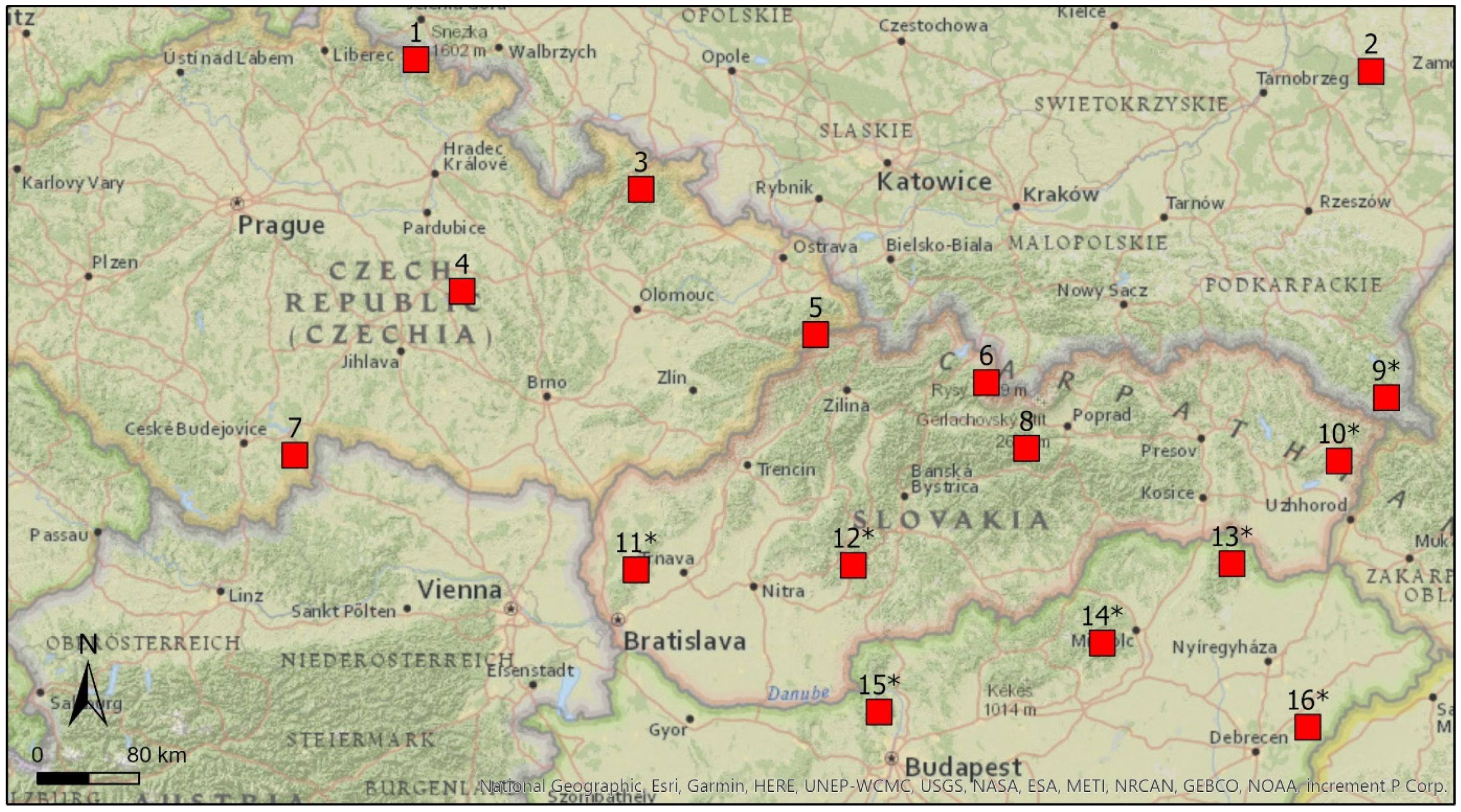
The relevance of the proposed LC-SLIAC method using C-band SAR satellite data was demonstrated in 16 study areas from different parts of Central Europe. The main task of the methodology was to explain the relationship between LIA and backscatter values by the calculation of regression line coefficients. Regression coefficients were also used in previous studies in the traditional pixel-based method (e.g., in [20,23,24]). They were calculated for each image pixel separately based on the backscatter and incidence angle values obtained from all available images in the selected time range. In this case, each pixel has its own unique regression coefficients. One of the disadvantages of the pixel-based regression method is that the number of different incidence angle values included in the regression analysis depends on the number of different satellite tracks available over the studied area. In the case of Central Europe, when using Sentinel-1 satellite data, there are only 2–4 satellite tracks available over a given area. In high latitude areas, where Sentinel-1 Extra-Wide (EW) swath data are available, it can be on average 4.9 to 7.7 tracks per pixel (e.g., in [26]). Some satellites can have more available different acquisition paths over the image pixel, i.e., in the case of Envisat with a maximum of 15 different available paths over an area in Germany (in [23]). However, the reasonable minimum sample size for regression analysis with one predictor should be ~50 based on the rule of thumbs (i.e., [50] or [51]). By using more measurements from the same path (i.e., from several acquisition times), the amount of data for each pixel can be larger (as used, e.g., in [23,24,25]), which results in several backscatter values for each individual incidence angle value. In this case, differences will appear only for the backscatter value caused mainly by the growing season or by changing climatic conditions during the year. In contrast, the regression line coefficients in the proposed LC-SLIAC method were calculated separately for each image from selected forest areas located in the SA. To get an appropriate number of forest points included in the regression analysis, these forest areas were selected from 1000 randomly generated points over the SA using the forest mask derived from a combination of CLC and GFC. On average, 395 forest points were included in the regression analysis (with a minimum of 138 and a maximum of 668 forest areas). From this point of view, each image has its unique regression coefficients. Therefore, the effect of different seasons (seasonality in data) through the year does not influence the coefficients. Combining the two land cover databases aimed to reduce the possibility of biasing the linear relationship by outliers that may represent non-forest areas due to errors in the land cover databases used. To reduce the possibility of selecting areas representing non-forest areas or forest pixels with a low density of trees, only pixels with at least 50% of tree canopy cover (from the GFC) were selected. The remaining outliers were excluded using Tukey’s fences. The accuracy assessment of the forest masks showed more than 90% overall accuracy of this approach.

The regression analyses performed on selected forest areas showed a negative linear relationship between backscatter and LIA for each SA. The negative linear behavior supports the existence of terrain effects on backscatter values and, therefore, reinforces the importance of its elimination. SAs with different terrain characteristics (i.e., mean elevation) and LIA characteristics (LIA range and LIA IQR) were used to compare the effect of LIA on backscatter for different types of SAs. Generally, stronger correlation, higher scale coefficient b and higher R² were found over more tilted SAs with high LIA range and LIA IQR. On the other hand, the mean elevation of selected forest areas has a lower influence on the obtained results. According to the found results, in SAs with relatively flat terrain (mean terrain slope <4°), with LIA range <22° and LIA IQR <4°, a low R² was observed (2–6%), and the regression was statistically not significant at the significance level of 1%. Excluding these SAs, the explained mean variation in backscatter by LIA was 55% and 58% for VV and VH polarization, respectively. The lowest R² of 15% (VH) was found in coniferous forests of Žďárské vrchy PLA with the lowest LIA range (29°) from the remaining SAs, and a maximum of 74% (VV) was found in coniferous forests of the Low Tatras NP (SA8) with the highest LIA range (66°). Achieved R² valeus are similar to results found in [52] (65% of the variation in backscatter was explained by terrain topography) and are higher than the results found in [53] (5–50%). In addition, these findings are in contrast with studies that found a nonlinear relationship between backscatter and LIA over a tilted terrain [12,27].

Slope coefficients b of the linear regression in this study were found to be steep and showed a relatively strong correlation in all SAs except low LIA SAs. Compared to earlier studies based on C-band data, i.e., to [28] or [29], a flat angular behavior was detected over forests (regression line slope b = 0.06), however in these studies, ERS-1 wind scatterometer data with a spatial resolution of 50 km was used, where it was almost impossible to avoid the mixed-pixel problem in the regression analysis. Linear regression line slope b in the presented study was higher than 0.2 dB/degree over Low and High Tatra NP (SA6 and SA8), with the highest LIA range and LIA IQR, while the lowest regression slope coefficient b was achieved in low LIA SAs. According to the comparison of the resulting statistics between coniferous and deciduous SAs after excluding low LIA SAs, the mean scale coefficient b and the coefficient of determination R² of coniferous forests were higher than for deciduous SAs by 0.02 dB/degree and ~5%, respectively. The influence of mean LIA range or LIA IQR was, in this case, minimal, as the difference between the two groups in the mean LIA range and LIA IQR was ~1°. These results correspond to the findings in [16], where higher values were also found for conifers. These findings also support the assumption for using the land cover-specific correction, that LIA has a different influence on backscatter based on the land cover class. Discrimination between coniferous and deciduous forests was found in previous studies (e.g., [21,52,54]). Higher obtained backscatter in VV polarization compared to VH over forested areas was found, which was also observed in earlier studies (i.e., [20,21,55]). It can be explained by the higher attenuation of VV polarization by vegetation cover compared to VH, as it was also found in [8].

It is shown in Figure 6 and Figure 7 that the LC-SLIAC method eliminates the effect of LIA on backscatter values. Statistical comparisons of uncorrected and corrected forest areas involved in the regression analysis showed a reduction in terms of backscatter variance after correction in all SAs. In low LIA SAs with gentle terrain slopes, the decrease in variance was very low and statistically not significant. High (>40% reduction with a maximum of 74%) and a statistically significant decrease in variance were found in all other areas, which are characterized as areas with moderate to steep terrain slopes. After the exclusion of low LIA SAs, other SAs showed the mean reduction in the variance of 56% and 60% for VH and VV polarization, respectively. That kind of reduction can be considered suitable for further analyses and is higher compared to earlier studies, where the terrain was considered moderate, and the cosine square correction or other methods were used—e.g., in [16], a maximum of 10% variance decrease after the correction was found, in [15] a decrease by 5–13% and in [40] a decrease of approximately 20% was found. However, the variance after the correction remained high (around 3.5 dB) in SAs with the most tilted terrain, while for other SAs, it was around 2 dB. The high variance of backscatter in the forest areas after correction can be caused by the generally high heterogeneity of forest vegetation (different types of trees, different growth stages, or density of trees involved in the regression analysis), which is especially higher at higher altitudes, as was also mentioned in [56].

The time-series analysis aimed to achieve better results using the mean LIA obtained from different paths, where the investigation was done only for the selected case study with its near surroundings (using a 20 m buffer). The validation of the proposed correction method applied in a three-month time-series analysis using all available Sentinel-1 satellite tracks showed that the LIA correction is the most effective and statistically significant in CSs, where the range of LIA ≥27° can be found. For CSs where the range of LIA ≤ 10°, the correction was almost not apparent, and the change in variance was statistically not significant, while for the CS9 with 27° LIA range was already statistically significant. Because only six CSs were tested for the effects of correction in this study, more CSs are needed to test in the future to identify a threshold LIA range at which the change is statistically significant using LC-SLIAC. These results are similar to the results in [16], where for pixels with LIA <26° and terrain slope <6° did not occur any considerable correction using semi-empirical cosine-based methods. Similarly, in the case of a different correction method used in [12], a minimal effect of the correction was found over areas with an incidence angle range <10°. However, after the correction, some fluctuations of values in the time-series remained using LC-SLIAC, which can be attributed to random short-term variations caused by environmental factors, like increased moisture or different reflectivity of the forest caused by different time of the acquisition (approximately 5 a.m. versus 5 p.m.). This different reflectivity can be caused, for instance, by change of temperature between two measurements, change in moisture, different nature of the leaves, etc. According to the influence of precipitation, Frison et al. [55] did not find any relationship between precipitation and backscatter values over forested areas using Sentinel-1 data. They explained this behavior by the difference between the measured precipitation and the precipitation that can be retained by the leaves or needles of a tree. Tanase et al. [57] found that C-band was less sensitive to vegetation water content (achieving variations about 1 dB) than the P- and L-bands.

Although there is an increasing number of studies using SAR data for time-series analyses of forests (e.g., in [21,55,58,59]), there is still a need for an interface and a tool, which is computationally not intensive and where multi-annual SAR time-series can be created. As the GEE is an open-access interface for non-commercial use, the LC-SLIAC method was implemented to the GEE and is available as a freely available function using the requirement call: require(‘users/danielp/LC-SLIAC:LC-SLIAC’).

A limitation of this study is that the methodology is prepared for application over forested areas. For the successful correction, an appropriate number of forest areas must be included in the regression analysis of backscatter and LIA. Therefore, the correction should be applied over areas with a higher share of forests. In the following studies, it would be appropriate to test and statistically evaluate the results in areas with different land cover types. Another limitation of this study is that the methodology was tested in countries of Central Europe, for which the CLC dataset is available. In the case of Europe, it will be worth trying to implement the Copernicus High-Resolution Layers for forests [60] or to test the method in countries out of the EU. It is possible to use other global, e.g., the Copernicus 100 m Copernicus Global Land Cover layers [61], regional, or national land cover databases. Instead of using land cover databases, it would also be useful to perform supervised classification on satellite data to determine the extent of forested areas in the studied area. In this study, a freely available DEM was used, i.e., the SRTM DEM with a 30 m resolution. Therefore, it will be important to test and validate the LC-SLIAC method using a more accurate and higher resolution DEM. Moreover, the simplified shadow and layover masking used in this study cannot consider the passive shadow and layover regions, which are important in eliminating non-valid pixels over tilted terrain.

There are still unanswered questions connected with this study. In future research, it is necessary to explain the reason for the short-term fluctuations of backscatter values in the subsequent dates, try to implement the methodology used in this study for long-term time-series to detect seasonality or changes in forests, as well as to understand the character of the seasonal activity, or in detail to access the relationship between radar time-series behavior and characteristics of the studied area (terrain slope, aspect, elevation, LIA range or characteristics of the vegetation). In the case of long-term time-series analysis, it should be helpful to implement radar indicators (e.g., polarimetric radar indices) to monitor the condition of forests and compare them with the most used vegetation indices (NDVI, NDMI) derived from optical data or test the impact of precipitation on the evaluation of long-term time-series and propose methods for their correction for C-band SAR data. On the other hand, the planned radar missions Biomass with P-band (2021), NISAR with L- and S-band (2022), TanDEM-L with the L-band (2022) can bring new opportunities for forest exploration and thus new challenges in data processing and analysis.

5. Conclusions

Remote sensing in the microwave electromagnetic spectrum has many advantages over optical data, e.g., daylight and weather-independent sensing. Since the launch of Sentinel-1 in 2014 with freely available SAR satellite data, new opportunities in forest monitoring have been opened to a wider research community. However, the interaction between the SAR signal and the surface is different from the equivalent interaction in optical remote sensing. Tilted terrain can have a strong influence on the resulting backscatter. In contrast, the influence is most pronounced in areas with steep slopes usually located at higher altitudes, especially when combining images from different orbits and paths for a time-series analysis (Figure 9a,b). Effects of the terrain need to be corrected before any further analysis over mountainous areas.

In this study, a method called LC-SLIAC was developed for SAR satellite data correction, mainly for time-series analysis of forests. LC-SLIAC was tested using Sentinel-1 C-band data in selected protected areas in Central Europe, followed by evaluating its relevance and accuracy. In this study, only open data were used: Sentinel-1, SRTM DEM, CORINE Land Cover, Hansen et al.’s Global Forest Change database, and freely available (for non-commercial use) cloud-based platform GEE. Based on the achieved results and their statistical evaluation, data after correction showed a reduction in statistical parameters (range, variance), which means a reduction of terrain-induced effects on backscatter values. In general, this method is useful over mountainous areas with moderate to steep sloping terrain, where the variation in LIA values for forests is high. In the short-term time series, data after correction showed smoother behavior (without apparent fluctuations caused by different LIAs) compared to uncorrected data. The reduction of variance in the time-series was by means up to 95%. The LC-SLIAC algorithm is freely available in the GitHub repository (https://github.com/palubad/LC-SLIAC, last accessed on 26 April 2021), and it is freely accessible for GEE users.

References

1. Amani, M.; Ghorbanian, A.; Ahmadi, S.A.; Kakooei, M.; Moghimi, A.; Mirmazloumi, S.M.; Moghaddam, S.H.A.; Mahdavi, S.; Ghahremanloo, M.; Parsian, S.; et al. Google Earth Engine Cloud Computing Platform for Remote Sensing Big Data Applications: A Comprehensive Review. IEEE J. Sel. Top. Appl. Earth Obs. Remote. Sens. 2020, 13, 5326–5350. [Google Scholar] [CrossRef]
2. Gorelick, N.; Hancher, M.; Dixon, M.; Ilyushchenko, S.; Thau, D.; Moore, R. Google Earth Engine: Planetary-Scale Geospatial Analysis for Everyone. Remote Sens. Environ. 2017, 202, 18–27. [Google Scholar] [CrossRef]
3. Ranson, K.J.; Kovacs, K.; Sun, G.; Kharuk, V.I. Disturbance Recognition in the Boreal Forest Using Radar and Landsat-7. Can. J. Remote Sens. 2003, 29, 271–285. [Google Scholar] [CrossRef]
4. Richards, J.A. Remote Sensing with Imaging Radar; Signals and Communication Technology; Springer: Berlin/Heidelberg, Germany, 2009; ISBN 978-3-642-02019-3. [Google Scholar]
5. Paloscia, S.; Santi, E.; Pettinato, S. Microwave Remote Sensing for the Monitoring of Forest Ecosystems-Presentation. 2015. Available online: https://www.gesaaf.unifi.it/upload/sub/eventi/4giugno2015/paloscia.pdf (accessed on 15 May 2020).
6. Patnaik, S.C. Basics of Microwave Data and Analysis for Forest Study. In Proceedings of the ERTD TREES Training-SAR & Hyperspectral Data Analysis for Forest Applications, Visulization of Earth observation Data and Archival System (VEDAS), Bengaluru, India, 30 October–3 November 2017; pp. 17–26. [Google Scholar]
7. Rüetschi, M.; Small, D.; Waser, L.T. Rapid Detection of Windthrows Using Sentinel-1 C-band SAR Data. Remote Sens. 2019, 11, 115. [Google Scholar] [CrossRef] [Green Version]
8. Yunjin, K.; van Zyl, J. Comparison of Forest Parameter Estimation Techniques Using SAR Data. In Proceedings of the IEEE 2001 International Geoscience and Remote Sensing Symposium (Cat. No.01CH37217), Sydney, NSW, Australia, 9–13 July 2001; Volume 3, pp. 1395–1397. [Google Scholar]
9. Li, J.; Wang, S. Using SAR-Derived Vegetation Descriptors in a Water Cloud Model to Improve Soil Moisture Retrieval. Remote Sens. 2018, 10, 1370. [Google Scholar] [CrossRef] [Green Version]
10. Olesk, A.; Voormansik, K.; Põhjala, M.; Noorma, M. Forest Change Detection from Sentinel-1 and ALOS-2 Satellite Images. In Proceedings of the 2015 IEEE 5th Asia-Pacific Conference on Synthetic Aperture Radar (APSAR), Singapore, 1–4 September 2015; Volume 2, pp. 522–527. [Google Scholar] [CrossRef]
11. Ranson, K.J.; Sun, G. Effects of Environmental Conditions on Boreal Forest Classification and Biomass Estimates with SAR. IEEE Trans. Geosci. Remote Sens. 2000, 38, 1242–1252. [Google Scholar] [CrossRef]
12. Mladenova, I.E.; Jackson, T.J.; Bindlish, R.; Hensley, S. Incidence Angle Normalization of Radar Backscatter Data. IEEE Trans. Geosci. Remote Sens. 2013, 51, 1791–1804. [Google Scholar] [CrossRef]
13. Topouzelis, K.; Singha, S. Incidence Angle Normalization of Wide Swath SAR Data for Oceanographic Applications. Open Geosci. 2016, 8, 450–464. [Google Scholar] [CrossRef] [Green Version]
14. Van Zyl, J.J. The Effect of Topography on Radar Scattering from Vegetated Areas. IEEE Trans. Geosci. Remote Sens. 1993, 2, 1132–1134. [Google Scholar] [CrossRef]
15. Bayer, T.; Winter, R.; Schreier, G. Terrain Influences in SAR Backscatter and Attempts to Their Correction. IEEE Trans. Geosci. Remote Sens. 1991, 29, 451–462. [Google Scholar] [CrossRef]
16. Hinse, M.; Gwyn, Q.H.J.; Bonn, F. Radiometric Correction of C-Band Imagery for Topographic Effects in Regions of Moderate Relief. IEEE Trans. Geosci. Remote Sens. 1988, 26, 122–132. [Google Scholar] [CrossRef]
17. Teillet, P.M.; Guindon, B.; Meunier, J.F.; Goodenough, D.G. Slope-Aspect Effects in Synthetic Aperture Radar Imagery. Can. J. Remote Sens. 1985, 11, 39–49. [Google Scholar] [CrossRef]
18. Zhou, C.; Zheng, L. Mapping Radar Glacier Zones and Dry Snow Line in the Antarctic Peninsula Using Sentinel-1 Images. Remote Sens. 2017, 9, 1171. [Google Scholar] [CrossRef] [Green Version]
19. Small, D. Flattening Gamma: Radiometric Terrain Correction for SAR Imagery. IEEE Trans. Geosci. Remote Sens. 2011, 49, 3081–3093. [Google Scholar] [CrossRef]
20. Dostálová, A.; Milenković, M.; Hollaus, M.; Wagner, W. Influence of Forest Structure on the Sentinel-1 Backscatter Variation-Analysis with Full-Waveform Lidar Data. In Living Planet Symposium 2016; ESA: Prague, Czech Republic, 2016; Volume SP-740. [Google Scholar]
21. Dostálová, A.; Wagner, W.; Milenković, M.; Hollaus, M. Annual Seasonality in Sentinel-1 Signal for Forest Mapping and Forest Type Classification. Int. J. Remote Sens. 2018, 39, 7738–7760. [Google Scholar] [CrossRef]
22. Gauthier, Y.; Bernier, M.; Fortin, J.P. Aspect and Incidence Angle Sensitivity in ERS-1 SAR Data. Int. J. Remote Sens. 1998, 19, 2001–2006. [Google Scholar] [CrossRef]
23. Nguyen, D.B.; Clauss, K.; Cao, S.; Naeimi, V.; Kuenzer, C.; Wagner, W. Mapping Rice Seasonality in the Mekong Delta with Multi-Year Envisat ASAR WSM Data. Remote Sens. 2015, 7, 15868–15893. [Google Scholar] [CrossRef] [Green Version]
24. Pathe, C.; Wagner, W.; Sabel, D.; Doubkova, M.; Basara, J.B. Using ENVISAT ASAR Global Mode Data for Surface Soil Moisture Retrieval over Oklahoma, USA. IEEE Trans. Geosci. Remote Sens. 2009, 47, 468–480. [Google Scholar] [CrossRef]
25. Loew, A.; Ludwig, R.; Mauser, W. Derivation of Surface Soil Moisture from ENVISAT ASAR Wide Swath and Image Mode Data in Agricultural Areas. IEEE Trans. Geosci. Remote Sens. 2006, 44, 889–898. [Google Scholar] [CrossRef]
26. Widhalm, B.; Bartsch, A.; Goler, R. Simplified Normalization of C-Band Synthetic Aperture Radar Data for Terrestrial Applications in High Latitude Environments. Remote Sens. 2018, 10, 551. [Google Scholar] [CrossRef] [Green Version]
27. Van Doninck, J.; Wagner, W.; Melzer, T.; De Baets, B.; Verhoest, N.E.C. Seasonality in the Angular Dependence of ASAR Wide Swath Backscatter. IEEE Geosci. Remote Sens. Lett. 2014, 11, 1423–1427. [Google Scholar] [CrossRef]
28. Frison, P.-L.; Mougin, E. Use of ERS-1 Wind Scatterometer Data over Land Surfaces. IEEE Trans. Geosci. Remote Sens. 1996, 34, 550–560. [Google Scholar] [CrossRef]
29. Mougin, D.; Lopes, A.; Frison, P.L.; Proisy, C. Preliminary Analysis of ERS-1 Wind Scatterometer Data over Land Surfaces. Int. J. Remote Sens. 1995, 16, 391–398. [Google Scholar] [CrossRef]
30. Vollrath, A.; Mullissa, A.; Reiche, J. Angular-Based Radiometric Slope Correction for Sentinel-1 on Google Earth Engine. Remote Sens. 2020, 12, 1867. [Google Scholar] [CrossRef]
31. Torres, R.; Snoeij, P.; Geudtner, D.; Bibby, D.; Davidson, M.; Attema, E.; Potin, P.; Rommen, B.Ö.; Floury, N.; Brown, M.; et al. GMES Sentinel-1 mission. Remote Sens. Environ. 2012, 120, 9–24. [Google Scholar] [CrossRef]
32. GEE Sentinel-1 Algorithms. Available online: https://developers.google.com/earth-engine/sentinel1 (accessed on 15 May 2020).
33. Farr, T.G.; Rosen, P.A.; Caro, E.; Crippen, R.; Duren, R.; Hensley, S.; Kobrick, M.; Paller, M.; Rodriguez, E.; Roth, L.; et al. The Shuttle Radar Topography Mission. Rev. Geophys. 2007, 45, RG2004. [Google Scholar] [CrossRef] [Green Version]
34. GEE SRTM Digital Elevation Data 30 m. Available online: https://developers.google.com/earth-engine/datasets/catalog/USGS_SRTMGL1_003#description (accessed on 14 May 2020).
35. Büttner, G.; Kosztra, B.; Soukup, T.; Sousa, A.; Langanke, T. CLC2018 Technical Guidelines; European Environment Agency: Wien, Austria, 2017; Volume 25, pp. 1–60. [Google Scholar]
36. Kosztra, B.; Büttner, G.; Hazeu, G.; Arnold, S. Updated CLC Illustrated Nomenclature Guidelines; European Environment Agency: Wien, Austria, 2019; pp. 1–126. [Google Scholar]
37. Hansen, M.C.; Potapov, P.V.; Moore, R.; Hancher, M.; Turubanova, S.A.; Tyukavina, A.; Thau, D.; Stehman, S.V.; Goetz, S.J.; Loveland, T.R.; et al. High-Resolution Global Maps of 21st-Century Forest Cover Change. Science 2013, 342, 850–853. [Google Scholar] [CrossRef] [Green Version]
38. Hansen, M.; Potapov, P.; Margono, B.; Stehman, S.; Turubanova, S.; Tyukavina, A. User Notes for Version 1.6 of Global Forest Change 2000–2018. Available online: http://earthenginepartners.appspot.com/science-2013-global-forest/download_v1.6.html (accessed on 13 May 2020).
39. Castel, T.; Beaudoin, A.; Stach, N.; Stussi, N.; Le Toan, T.; Durand, P. Sensitivity of Space-Borne SAR Data to Forest Parameters over Sloping Terrain. Theory and Experiment. Int. J. Remote Sens. 2001, 22, 2351–2376. [Google Scholar] [CrossRef]
40. Franklin, S.E.; Lavigne, M.B.; Hunt, E.R.; Wilson, B.A.; Peddle, D.R.; McDermid, G.J.; Giles, P.T. Topographic Dependence of Synthetic Aperture Radar Imagery. Comput. Geosci. 1995, 21, 521–532. [Google Scholar] [CrossRef]
41. Ulander, L.M.H. Radiometrie Slope Correction of Synthetic-Aperture Radar Images. IEEE Trans. Geosci. Remote Sens. 1996, 34, 1115–1122. [Google Scholar] [CrossRef]
42. Paluba, D. A Correction of the Local Incidence Angle of SAR Data: A Land Cover Specific Approach for Time Series Analysis. Master’s Thesis, Charles University, Prague, Czech Republic, 2020. [Google Scholar] [CrossRef]
43. Lemoine, G. Sentinel-1-Local Incidence Angle Discussion on GEE Forum. Available online: https://groups.google.com/g/google-earth-engine-developers/c/cO0o2yoGdr0/m/oH3Y-LBJCgAJ (accessed on 11 March 2021).
44. Colesanti, C.; Wasowski, J. Investigating Landslides with Space-Borne Synthetic Aperture Radar (SAR) Interferometry. Eng. Geol. 2006, 88, 173–199. [Google Scholar] [CrossRef]
45. Kaasalainen, S.; Hyyppä, J.; Karjalainen, M.; Krooks, A.; Lyytikainen-Saarenmaa, P.; Holopainen, M.; Jaakkola, A. Comparison of Terrestrial Laser Scanner and Synthetic Aperture Radar Data in the Study of Forest Defoliation. In Proceedings of the ISPRS TC VII Symposium–100 Years ISPRS, Vienna, Austria, 5–7 July 2010; Wagner, W., Székely, B., Eds.; International Society for Photogrammetry and Remote Sensing: Vienna, Austria, 2010; Volume 38. [Google Scholar]
46. Rauste, Y.; Antropov, O.; Mutanen, T.; Häme, T. On Clear-Cut Mappingwith Time-Series of Sentinel-1 Data in Boreal Forest. In Proceedings of the Living Planet Symposium 2016, Prague, Czech, 9–13 May 2016; Volume SP-740, pp. 9–13. [Google Scholar]
47. Vreugdenhil, M.; Wagner, W.; Bauer-Marschallinger, B.; Pfeil, I.; Teubner, I.; Rüdiger, C.; Strauss, P. Sensitivity of Sentinel-1 Backscatter to Vegetation Dynamics: An Austrian Case Study. Remote Sens. 2018, 10, 1396. [Google Scholar] [CrossRef] [Green Version]
48. Reiche, J.; Mullissa, A.; Slagter, B.; Gou, Y.; Tsendbazar, N.E.; Odongo-Braun, C.; Vollrath, A.; Weisse, M.J.; Stolle, F.; Pickens, A.; et al. Forest Disturbance Alerts for the Congo Basin Using Sentinel-1. Environ. Res. Lett. 2021, 16. [Google Scholar] [CrossRef]
49. Reiche, J.; Herold, M.; Mullissa, A.; Gou, Y.; Slagter, B.; Tsendbazar, N.E. RADD Forest Disturbance Alert. Available online: https://www.wur.nl/en/Research-Results/Chair-groups/Environmental-Sciences/Laboratory-of-Geo-information-Science-and-Remote-Sensing/Research/Sensing-measuring/RADD-Forest-Disturbance-Alert.htm (accessed on 14 April 2021).
50. Green, S.B. How Many Subjects Does It Take To Do A Regression Analysis. Multivar. Behav. Res. 1991, 26, 499–510. [Google Scholar] [CrossRef] [PubMed]
51. Harris, R.J. A Primer of Multivariate Statistics, 2nd ed.; Academic Press: New York, NY, USA, 1985. [Google Scholar]
52. RAUSTE, Y. Incidence-Angle Dependence in Forested and Non-Forested Areas in Seasat SAR Data. Int. J. Remote Sens. 1990, 11, 1267–1276. [Google Scholar] [CrossRef]
53. Foody, G.M. An Assessment of the Topographic Effects on SAR Image Tone. Can. J. Remote Sens. 1986, 12, 124–131. [Google Scholar] [CrossRef]
54. Ranson, K.J.; Sun, G. Northern Forest Classification Using Temporal Multifrequency and Multipolarimetric SAR Images. Remote Sens. Environ. 1994, 47, 142–153. [Google Scholar] [CrossRef]
55. Frison, P.L.; Fruneau, B.; Kmiha, S.; Soudani, K.; Dufrêne, E.; Le Toan, T.; Koleck, T.; Villard, L.; Mougin, E.; Rudant, J.P. Potential of Sentinel-1 Data for Monitoring Temperate Mixed Forest Phenology. Remote Sens. 2018, 10, 2049. [Google Scholar] [CrossRef] [Green Version]
56. Pairman, D.; Belliss, S.E.; McNeill, S.J. Terrain Influences on SAR Backscatter Around Mt. Taranaki, New Zealand. IEEE Trans. Geosci. Remote Sens. 1997, 35, 924–932. [Google Scholar] [CrossRef]
57. Tanase, M.A.; Villard, L.; Pitar, D.; Apostol, B.; Petrila, M.; Chivulescu, S.; Leca, S.; Borlaf-Mena, I.; Pascu, I.S.; Dobre, A.C.; et al. Synthetic Aperture Radar Sensitivity to Forest Changes: A Simulations-Based Study for the Romanian Forests. Sci. Total. Environ. 2019, 689, 1104–1114. [Google Scholar] [CrossRef]
58. Proisy, C.; Mougin, E.; Dufrêne, E.; Le Dantec, V. Monitoring Seasonal Changes of a Mixed Temperate Forest Using ERS SAR Observations. IEEE Trans. Geosci. Remote Sens. 2000, 38, 540–552. [Google Scholar] [CrossRef]
59. Bouvet, A.; Mermoz, S.; Ballère, M.; Koleck, T.; Le Toan, T. Use of the SAR Shadowing Effect for Deforestation Detection with Sentinel-1 Time Series. Remote Sens. 2018, 10, 1250. [Google Scholar] [CrossRef] [Green Version]
60. EEA. Copernicus Land Monitoring Service: High Resolution Land Cover Characteristics-Tree-Cover/Forest and Change 2015–2018. 2020. Available online: https://land.copernicus.eu/pan-european/high-resolution-layers (accessed on 5 March 2021).
61. Buchhorn, M.; Lesiv, M.; Tsendbazar, N.E.; Herold, M.; Bertels, L.; Smets, B. Copernicus Global Land Cover Layers-Collection 2. Remote Sens. 2020, 12, 1044. [Google Scholar] [CrossRef] [Green Version]
Figure 1. Map of study areas. Study areas marked with * are areas with majority of deciduous forests.
Remotesensing 13 01743 g001
Figure 2. Methodology workflow used in this work.
Remotesensing 13 01743 g002
Figure 3. Difference between radar incidence angle (θ) and local incidence angle (θ0). LS = local slope.
Remotesensing 13 01743 g003
Figure 4. Illustration of the incidence wave vector i dependence on the vector normal to the surface n—angles and points involved in the computation of the LIA. RLA = radar look angle (the projection of the incidence plane).
Remotesensing 13 01743 g004
Figure 5. Boxplots of LIA for forest areas in the study areas. Boxplots represent the interquartile range and the lower and upper ranges. Study areas marked with * are areas with majority of deciduous forests.
Remotesensing 13 01743 g005
Figure 6. Comparison of relationships between VH and LIA for forest areas in the coniferous forest in Krkonoše NP, Czechia (SA1) before and after the correction for Sentinel-1B satellite data for 2018-06-02.
Remotesensing 13 01743 g006
Figure 7. Statistics of backscatter for selected forest areas within each SA from the linear regression analysis before and after the LIA correction. Study areas with dashed lines represent deciduous forests.
Remotesensing 13 01743 g007
Figure 8. Comparison of backscatter and LIA values for case study 8.
Remotesensing 13 01743 g008
Figure 9. Short-term time-series analysis of corrected and uncorrected data for selected case studies with different LIA ranges.
Remotesensing 13 01743 g009